Empirical Validation of Bimodal MFD Models

1. Introduction

The concept of Macroscopic Fundamental Diagram (MFD) was first proposed by Godfrey (1969) and later revisited by Mahmassani et al. (1984) in the context of simulations. It relates the density of vehicles to the mean flow at the network level. The existence of empirical MFD was shown a not long time ago by Geroliminis and Daganzo (2008) for the city of Yokohama, Japan. Ever since, there had been several applications like traffic state estimation (Yildirimoglu and Geroliminis, 2014; Kavianipour et al., 2019), perimeter control (Keyvan-Ekbatani et al., 2012; Ampountolas et al., 2017; Haddad and Mirkin, 2017; Mohajerpoor et al., 2020), route guidance (Genser and Kouvelas, 2020), congestion pricing (Gu et al., 2018), and cruising for parking (Cao and Menendez, 2015; Leclercq et al., 2017), etc. proposed based on MFD approach at the network level.

Most of the approaches proposed in the literature are based on the so-called uni-modal or 2D-MFD, which relates the accumulation of all vehicles to the mean flow of all vehicles in the network. Previous works (e.g., Boyac and Geroliminis, 2011; Chiabaut et al., 2014; Loder et al., 2017, 2019), suggest that the buses and cars affect the network dynamics in different ways. This phenomenon is clear in any urban network as public transport buses typically travel slower than cars and make frequent stops. At the same time, buses making stops may slow down car traffic, especially at on-street stops. The 2D-MFD approach may be too crude to properly consider the behavior of each transportation mode and their interactions. Geroliminis et al. (2014) was the first to address this issue by proposing a bi-modal or 3D-MFD for the area of downtown San Francisco using micro-simulations. This so-called 3D-MFD for bi-modal traffic data relates the accumulation of cars, buses to the total mean flow in the network. Ortigosa et al. (2015) calibrated 3D-MFDs for the cities of Zurich and San Francisco based on micro-simulations to study the influence of dedicated bus lanes on the urban networks. Following, Loder et al. (2017) presented the first experimental proof of the existence of a well-defined 3D-MFD for two different regions in Zurich. The Loop Detector Data (LDD) was fused with the public transport data recorded by Automatic Vehicle Location (AVL) devices to estimate both accumulations of cars and buses and overall travel production, i.e., total travel distance per unit of time. More recently, Huang et al. (2019) investigated the existence of 3D-MFD using the GPS data of private cars, taxis and public buses for the city of Shenzhen in China.

Two types of MFD-based models are primarily used in the literature, namely, accumulation-based and trip-based models. Accumulation-based model (Daganzo, 2007; Geroliminis, 2009; Yildirimoglu et al., 2015) is computationally more efficient, however it suffers from few drawbacks as illustrated in Mariotte et al. (2017). On the other hand, trip-based model (Arnott, 2013; Daganzo and Lehe, 2015; Lamotte and Geroliminis, 2016; Leclercq et al., 2017) is computationally more demanding, which addresses the shortcomings of the accumulation-based model in the free-flow regime. As the empirical evidence of 3D-MFD existence was established in the literature, it was necessary to extend the existing MFD-based modeling framework to multi-modal networks. The previous work of the authors (Paipuri and Leclercq, 2020) investigated this research question by studying the existing MFD-based modeling framework when used in conjunction with 3D-MFD. Besides the conventional MFD-based models, the authors revisited the accumulation-based model with outflow delay in the stated work.

The present work is essentially the continuation of the previous work of the authors, where the proposed MFD-based models founded on 3D-MFD are validated using empirical data. The authors of Loder et al. (2017) kindly shared the data they used to present the 3D-MFDs of two regions in Zurich. It happens that they have at their disposal the time series of the multi-modal network stats (accumulation and production per vehicle category) that have not been processed yet. Note that this type of data is challenging to collect in the real-world. The three primary prerequisites for performing an MFD-based simulation in a single reservoir are (i) underlying MFD (ii) inflow demand and (iii) trip lengths. It is to be noted that there is no available data on the inflow demand to the considered regions nor the trip length data. Therefore, approximation methods are proposed in the present work to estimate the inflow demand and trip lengths from the available data. Thus, the main contributions of the current work are the calibration of 3D-MFD shape and the validation of bi-modal MFD-based models using empirical data. The objective of this work is to highlight that the proper calibration of the 3D-MFD leads to the accurate reproduction of the dynamic traffic state in the network. Based on this, it is possible to test other scenarios corresponding to various demand profiles (for example, implementing new demand management strategies) and use the model predictions to assess different traffic management strategies.

The remainder of the manuscript is organized as follows: section 2 presents the empirical data for the 3D-MFD, section 4 details the inflow demand estimation techniques, section 5 illustrates the trip length estimation method, section 6 discusses the results and finally, section 7 presents the conclusions of the work.

2. Empirical Data

Figure 1 shows the regions of City center and Wiedikon in Zurich, Switzerland that are considered in the present work along with their link-level representations. There are 1,115 number of nodes and 3,046 number of edges in the City center, whereas in Wiedikon the number of nodes and edges are 2,264 and 5,879, respectively. It was also mentioned in Loder et al. (2017) that the regions were selected based on the homogeneity requirements and hence, no further partitioning is made in the present work. Empirical data is available as time series data of accumulations and productions for private cars and public transport vehicles for 1 week. However, no data are available concerning the trajectories of the vehicles nor inflow demand. Figures 2A,B show the corresponding empirical 3D-MFDs estimated from 26th to 30th October 2015 from 06:00 to 24:00 on each day. It is worth noting that the empirical data presented in Figure 2 corresponds to the production of private cars (P_c) only and public transport vehicles are excluded. It is discussed later about the rationale of choosing only private cars 3D-MFD.

FIGURE 1

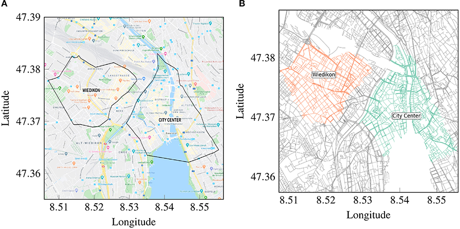
Figure 1. The partitions of City center and Wiedikon considered in the present work in the city of Zürich, Switzerland. (A) City center and Wiedikon areas © Google Maps 2020, (B) link level representations.

FIGURE 2

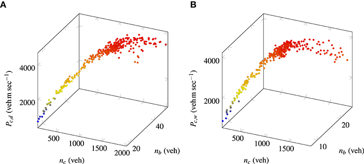
Figure 2. Empirical 3D MFDs for the considered regions. (A) City Center, (B) Wiedikon.

Figures 3A,B present the evolution of accumulations and mean speeds of private cars in the City center and Wiedikon, respectively. Each line of a given color corresponds to a different weekday in that region. Several observations can be inferred from the evolution plots. The morning peak hour is not very well-defined in the City center, where the peak accumulations and time of their occurrence vary for each day. On the contrary, the morning peak for the Wiedikon is relatively stable, where all days converge to the same peak accumulation. The peak accumulations in the evening peak hour vary day-to-day for both City center and Wiedikon regions. It is evident from the plots that the peak accumulation at the evening peak period is substantially higher than that of the morning peak for the Wiedikon region. This higher accumulation can be due to supply limitations (internal bottlenecks or congestion spreading from outside the perimeter) in the region during the peak period. Moreover, it can be noticed that there are few data points on the congestion branch of 3D-MFD for Wiedikon shown in Figure 2B indicating there are indeed supply limitations. These observations are valid for the mean speed evolution too.

FIGURE 3

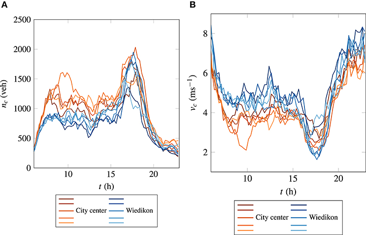
Figure 3. Empirical data of City center and Wiedikon regions. (A) Accumulation, (B) mean speed.

In order to fit the empirical data, the same functional form proposed by Loder et al. (2017) is used as a first step. The mean speed of cars is expressed as a linear combination of the accumulation of private cars and public transport vehicles. It can be expressed as,

$\begin{array}{ll}{v}_{c,r}=v_{c,r}^f+{\beta }_{c,r}{n}_{c,r}+{\beta }_{b,r}{n}_{b,r},& (1)\end{array}$

where subscripts c stands for private cars and r is the region under consideration. In the present context, the City center and Wiedikon are denoted by d and w, respectively. Similarly, $v_{c,r}^f$ is the free-flow speed (in m s-1) of private cars in the region r, n_c,r and n_b,r are the accumulations of private cars and public transport vehicles (in veh) in the region r, respectively. Finally, β_c,r and β_b,r are the constants of the fit. As briefed in the stated work, this type of functional form has a clear physical interpretation, i.e., constants of the fit indicate the negative marginal effect of each mode on the mean speed of private cars. Table 1 shows the fit coefficient values obtained by the least-squares method. Even though this functional form results in a relatively good fit, with R² = 0.954 for the City center, it will be shown later that the fit does not reproduce the traffic dynamics, i.e., the production and accumulation time series, accurately in the context of MFD-based framework. This is due to the constant first-order derivative, which oversimplifies the mean speed evolution. This limitation can be addressed by considering either higher-degree terms in the functional form of mean speed evolution or exponential type of functional form proposed in Geroliminis et al. (2014).

TABLE 1

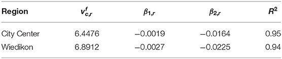
Table 1. Fit parameters of bi-linear functional form for City center and Wiedikon regions.

Considering higher degree terms in the functional form do not result in a concave-shaped 3D-MFD. At the same time, it was proposed in Geroliminis et al. (2014) that the mean speed fit must be estimated considering certain constraints on the fit coefficients in order to be consistent with the physics of traffic. However, it is noticed in the current work that such constraints can yield a poor quality fit in the context of the prediction of traffic state variables. Hence, the bi-linear functional form presented in Equation (1) is used in the present work. It will be demonstrated using the validation results in section 6 the limitations of using a single 3D-MFD and how it can be appropriately addressed.

From Table 1, it is clear that the free-flow speed of Wiedikon is slightly higher than the City center. This can be due to the longer links and fewer signaled intersections in Wiedikon. The R² values indicates that relatively tight fits are obtained for both fits. Figure 4 shows the contour plots of the estimated fits presented in Table 1 along with the empirical data for the City center and Wiedikon. In the present analysis, the bounds on accumulations, i.e., $\left\{n_{c,d}^{\mathrm{\text{max}}},n_{b,d}^{\mathrm{\text{max}}}\right\}=\left\{2200,60\right\}$ for the City center and $\left\{n_{c,w}^{\mathrm{\text{max}}},n_{b,w}^{\mathrm{\text{max}}}\right\}=\left\{2000,40\right\}$ for the Wiedikon.

FIGURE 4

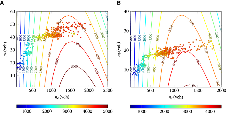
Figure 4. Estimated fits and empirical data for the considered regions. (A) City Center, (B) Wiedikon.

As already stated, no OD matrix data is available to the authors for the city of Zurich. Hence, inflow demand for both regions under consideration is unknown and it must be estimated. At the same time, the mean trip lengths inside each region are also unknown. On the one hand, estimating the average trip length and inflow demand of the public transport vehicles is feasible, as they have fixed routes and schedules. On the other hand, estimating the average trip lengths of private cars is far from trivial. It is impossible to estimate the trip lengths of the vehicles using LDD without any additional equipment. Recently, Barmpounakis and Geroliminis (2020) proposed a framework for urban monitoring using hovering drones, where trajectories of all individual vehicles can be extracted from the data. Paipuri et al. (2020) demonstrated the estimation of various MFD-based modeling parameters, including trip lengths using mobile phone data. Therefore, a massive amount of data is needed to estimate the trip lengths in an urban region. In order to address these shortcomings, a more straightforward approach to the validation is adopted in the present work.

It is also worth noting that the prediction of the number of public transport vehicles that are circulating in the network is straightforward, as they have fixed schedules and AVL devices can be used to extract this information in real-time. However, predicting the number of private vehicles circulating in the network at any given time is less trivial. Moreover, accurate prediction of this variable is crucial for applications like perimeter control. Hence, the number of private vehicles circulating in the network can be considered as the primary variable of interest. In the present work, the accumulation of public transport vehicles is used as an input to the MFD-based models. Thus, the traffic state evolutions of private vehicles are compared with empirical data to validate the models. This is the reason for choosing empirical 3D-MFD of private cars only and excluding public transport vehicles.

3. MFD-Based Models

In this work three MFD-based models are used namely: accumulation-based, trip-based and accumulation-based with outflow delay. Accumulation-based model uses conservation equation to resolve the reservoir dynamics given as follows,

$\begin{array}{ll}\frac{\text{d}{n}_{c,r}(t)}{\text{d}t}=q_{\text{in},c,r}(t)-q_{\text{out},c,r}(t),& (2)\end{array}$

where n_c,r is accumulation of private cars in region r, q_in,c,r and q_out,c,r are inflow and outflow, respectively. Forward Euler scheme is used to discretize this Ordinary Differential Equation (ODE), which yields as follows,

$\begin{array}{ll}{n}_{c,r}^{t+1}-n_{c,r}^t=\Delta t\left({\lambda }_{\text{in},c,r}^t-\frac{P_{c,r}(n_{c,r}^t,n_{p,r}^t)}{L_{c,r}}\right),& (3)\end{array}$

where Δt is time step, ${\lambda }_{\mathrm{\text{in}},c,r}^t$ is inflow demand for private cars at time t in region r, accumulations of private cars and public transport vehicles at time t are denoted by $n_{c,r}^t$ and $n_{p,r}^t$, respectively and finally, L_c,r is the mean trip length for private cars inside the region r. Note that inflow is assumed to be known a priori in the current context and hence, no entry flow function is considered. At all time instants, $q_{\mathrm{\text{in}},c,r}={\lambda }_{\mathrm{\text{in}},c,r}^t$. Outflow is computed from the private cars 3D-MFD as $\frac{P_{c,r}(n_{c,r}^t,n_{p,r}^t)}{L_{c,r}}$. Accumulation of public transport vehicles, $n_{p,r}^t$, is provided to the model as an input and accumulation of private cars, $n_{c,r}^t$, is known at time t. Thus, using these two traffic state variables, travel production of the private cars can be computed using fit functional forms discussed in previous section. Moreover, it was already shown in Paipuri and Leclercq (2020) that using partial 3D-MFDs improve the accuracy of the models and hence, only partial 3D-MFD of private cars is considered.

Now considering the trip-based formulation, mathematically it can be expressed as,

$\begin{array}{ll}{L}_{c,r}={\displaystyle {\int }_{t-{\tau }_{c,r}(t)}^t}{v}_{c,r}(n_{c,r}(s),n_{p,r}(s))\text{ d}s,& (4)\end{array}$

where τ_c,r(t) is the travel time of private cars at time t in region r. The mean speed at each time instant depends on the accumulations of private cars and public transport vehicles, which is given by velocity 3D-MFD, v_c,r. The trip starting times of all vehicles are computed based on the inflow demand. The vehicles leave the reservoir once they travel their assigned trip lengths L_c,r. During the course of the trip, the mean speed is updated whenever there is an entry or exit of a vehicle.

The outflow is delayed by the order of travel time at any time instance, t in the delay accumulation-based model. This model was first introduced by Friesz et al. (1989) and Ran et al. (1993) in the context of link level traffic dynamics and later used by Haddad and Zheng (2018) and Zhong et al. (2018) in the context of MFD-based modeling. The delayed outflow of private cars in region r can be expressed as,

$\begin{array}{ll}{q}_{\text{out},c,r}(t+{\tau }_{c,r}(t))=\frac{q_{\text{in},c,r}(t)}{1+\frac{\text{d}{\tau }_{c,r}(t)}{\text{d}t}},& (5)\end{array}$

where, $\frac{\text{d}{\tau }_{c,r}(t)}{\text{d}t}$ can be computed as follows,

$\begin{array}{l}\frac{\text{d}{\tau }_{c,r}(t)}{\text{d}t}=\frac{\partial {\tau }_{c,r}}{\partial n_{c,r}}(q_{\text{in},c,r}(t)-q_{\text{out},c,r}(t))\\ +\frac{\partial {\tau }_{c,r}}{\partial n_{c,r}}\frac{n_{p,r}(t+\Delta t)-n_{p,r}(t)}{\Delta t}.& (6)\end{array}$

The travel time function can be obtained from the velocity 3D-MFD, i.e., ${\tau }_{c,r}(n_{c,r},n_{p,r})=\frac{L_{c,r}}{v(n_{c,r},n_{p,r})}$. The formulations and numerical resolutions of various models are discussed in-detail in Paipuri and Leclercq (2020). In the following sections, inflow demand and trip lengths estimation methods are discussed in detail.

4. Re-construction of Inflow Demand From Empirical Data

As explained earlier the bi-modal model is solved for the accumulation of private cars only and therefore, it is enough to re-construct the inflow demand for the private cars. Note that this does not mean that the effect of public transport vehicles on private car traffic is neglected. Both traffic modes are indeed considered but, number of circulating public transport vehicles is given as input to the model as illustrated in section 3. This differs from the general expression of bi-modal MFD models, where accumulations of both modes are simultaneously computed using the bi-modal inflow demand (Paipuri and Leclercq, 2020). The current approach of re-constructing inflow demand is based on the inflow and outflow cumulative curves. They can be expressed as,

$\begin{array}{ll}\begin{array}{c}{N}_{\text{in},c,r}={\displaystyle \int }{q}_{\text{in},c,r}\text{ d}t,\\ N_{\text{out},c,r}={\displaystyle \int }{q}_{\text{out},c,r}\text{ d}t,\end{array}& (7)\end{array}$

where q_in,c,r and q_out,c,r are inflow and outflow for region r, respectively. The variables N_in,c,r(t) and N_out,c,r(t) indicate cumulative number of vehicles entered and exited the region at time t. The outflow in the present context corresponds to the sum of outflow of vehicles that leave the region and trip completion rate of vehicles that have destinations inside the region. This outflow can be computed from partial production of private cars, P_c,r, as follows,

$\begin{array}{ll}{q}_{\text{out},c,r}=\frac{P_{c,r}}{L_{c,r}},& (8)\end{array}$

where L_c,r is the mean trip length of all trajectories of private cars in region r. The estimation of mean trip length is discussed in the next section and thus, it is assumed to be a known here. Using the estimated mean trip length and partial production of private cars, trip completion rate and outflow cumulative curve can be estimated using Equations (8) and (7), respectively. If a vehicle i enters the region at time $t_i^e$ and leaves at $t_i^s$, then it is evident from the concept of cumulative curves that $N_{\mathrm{\text{in}},c,r}(t_i^e)=N_{\mathrm{\text{out}},c,r}(t_i^s)$. Thus, N_out,c,r at time $t_i^s$ must be projected to N_in,c,r at time $t_i^e$ to estimate N_in,c,r. Once N_in,c,r is computed, q_in,c,r can be estimated using Equation (7). Since N_out,c,r is known at every time step $t_i^s$, the only remaining unknown to compute N_in,c,r is $t_i^e=t_i^s-T{T}_i$, where TT_i is the travel time. For sake of simplicity, the subscripts (c,r) are omitted for the rest of the section.

Empirical data does not contain the travel time of each vehicle. However, data has the evolution of mean speed with time inside each region (City center and Wiedikon). According to the hypothesis of the MFD-based framework, all vehicles travel at the same speed given by the MFD at any given time. Hence, it is possible to extract the travel time of each vehicle from the mean speed evolution graphically. Two different approaches can be adopted in this context. Figure 5A presents sample inflow and outflow cumulative counts. As stated earlier, consider a vehicle i finishes the trip at time $t_i^s$. It is possible to obtain the mean speed of all vehicles at that time from the evolution of mean speed shown in the inset plot. Although mean speed changes during the trip, for the sake of simplicity, constant mean speed at time $t_i^s$ can be assumed to be the mean speed throughout the trip. By this approximation, the travel time of the vehicle i can be computed using trip length L and mean speed $v_i^s$. It can be argued that this method has a strong assumption of constant mean speed throughout the trip and introduces a heavy bias in the computation of inflow demand. Hence, an alternate approach is proposed in this work to calibrate the inflow demand more accurately.

FIGURE 5

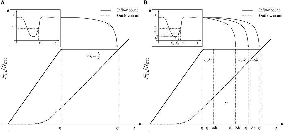
Figure 5. Approximation methods to calibrate inflow cumulative curve. (A) Constant mean speed, (B) variable mean speed.

Figure 5B illustrates the second approach. The principal idea is to consider variable mean speed instead of constant mean speed throughout the trip. The time axis is discretized with a step δt to account for the variability in the mean speed. Assuming the trip completion time of vehicle i as $t_i^s$, the preceding time steps are $t_{i,1}^s=t_i^s-\delta t$, $t_{i,2}=t_i^s-2\delta t$ and so on. If $v_i^s$ is the mean speed at time $t_i^s$, it can be safely assumed that the mean speed between $t_i^s$ and $t_i^s-\delta t$ is $v_i^s$. Therefore, the distance traveled during the first time step is $v_i^s\delta t$. If $v_{i,1}^s$ and $v_{i,2}^s$ are the mean speeds at $t_{i,1}^s$ and $t_{i,2}^s$, distances traveled during those time periods are v_i,1δt and v_i,2δt, respectively. Graphically, it is clear that the travel time at $t_i^s$ is nδt, where n corresponds to number of time steps that gives sum of distances traveled in each time step equal to the trip length. Mathematically, it can be expressed as,

$\begin{array}{ll}T{T}_i=n\delta t\text{ where }n=\underset{i\in \mathbb{Z}}{\text{argmin}}\left({\displaystyle \sum _i}(v(t-i\delta t)\delta t)-L\right),& (9)\end{array}$

where v(t) is the mean speed function. This approach takes the variability of the mean speed into account. However, it is to be noted that the accuracy gained in this approach depends on the resolution of empirical data of the mean speed. In the present work, mean speed data is only available for every 15 min aggregation interval. This is a relatively long period and it is noticed that the inflow cumulative curves calibrated using both approaches resulted in a very similar evolution.

Once the inflow cumulative curve is estimated, the inflow demand can be computed by taking the first-order derivative of the cumulative curve. It should be noted that both of the presented approaches are only approximation of inflow demand and it is not possible to segregate the internal and transfer demands for each region under consideration. However, it is noticed from the results that in the absence of relevant data, this approach gives a satisfactory inflow demand for the bi-modal MFD-based model. Figure 6 presents the estimated inflow demand for the City center and Wiedikon. It can be observed that the inflow demand profiles have high variability, especially during peak and off-peak periods.

FIGURE 6

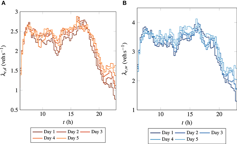
Figure 6. Estimated inflow demand patterns. (A) City center, (B) Wiedikon.

It can be argued that using the same data to estimate the inflow demand profile and assessing the accuracy of MFD-based simulation can result in a degree of over-fitting. However, it will be shown in section 6 that an improper calibration of 3D-MFD fit can result in erroneous traffic state dynamics, even with well-estimated inflow demand. This study highlights the importance of calibration of 3D-MFD fit and it is only possible if the errors from inflow and trip length estimation are minimized. Moreover, different demand scenarios can be studied in the context of implementing demand management strategies with an accurately calibrated 3D-MFD fit. The proposed inflow estimation method can be compared with loop detector data at the perimeter in-bounds of the region, if available. Total inflow traffic counts can be estimated; however, they cover only a fraction of links in the region. Hence, the traffic counts on these selected links need to be expanded to the entire region by using some metric of expansion factor. Estimating this expansion or scaling factor is not straightforward and can introduce bias in the macroscopic traffic variables. Yet, this study cannot be realized in the current context as data is available only in the form of aggregated loop observations and not individual ones.

5. Trip Lengths Estimation

As already mentioned, there is no available empirical data on the trip lengths inside each region. Therefore for estimating trip lengths, a network exploration technique (Batista et al., 2019) is used. A similar method can be used to estimate the dynamic trip lengths as illustrated in Batista et al. (2020). This technique involves randomly generating numerous local trips in the network and estimating the mean trip lengths from this generated set of trips. Two essential tools are used in this context, namely, OSMnx (Boeing, 2017), which is a Python package used to analyze the road networks and NetworkX (Hagberg et al., 2008), another Python package used to study the dynamics of road networks.

Origins are randomly generated, 2,000 in the present work, for the whole city of Zurich. Figure 7A shows the origin points generated for the whole network. Since the locations of these randomly generated origins not necessarily lie on the road network, the nearest nodes to each origin point are estimated as a first step. Following, the shortest paths between all these OD pairs are computed and they are assumed to be trip patterns in the network. Figure 7B presents a sample trip set generated between the OD pairs. The trips that go across the considered regions are highlighted in colors. Now, all the trips that transverse through the considered regions are clustered to estimate an average trip length inside each region. Approximately, a total of 3.8 million trips are sampled across the whole network, of which 1 million trips transverse each region. Figure 8 presents the distribution of trip lengths obtained by the network exploration technique in the City center and Wiedikon regions. These distributions yield average trip lengths of 1 550 m and 980 m in the City center and Wiedikon, respectively. The total lengths for the car network in the City center and Wiedikon are 39 and 31 km, respectively. Hence, by comparing the ratio of estimated trip lengths and total network lengths for two regions, it can be concluded that the obtained average trip lengths are representative.

FIGURE 7

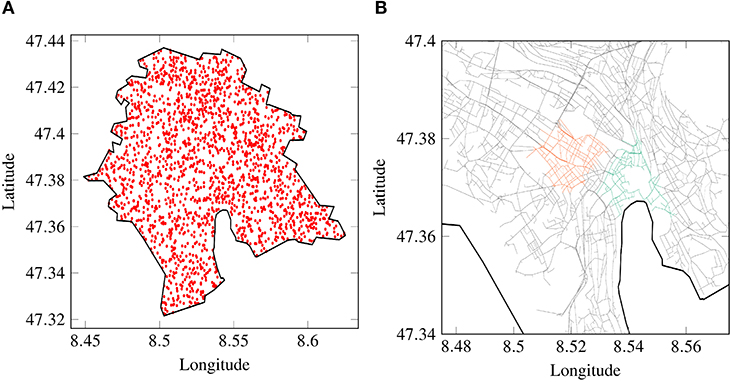
Figure 7. Network exploration technique. (A) Randomly generated origins, (B) sample set of trips.

FIGURE 8

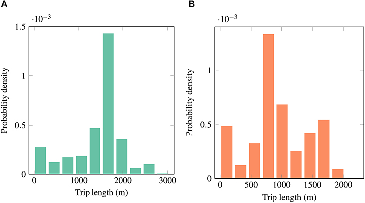
Figure 8. Distribution trip lengths. (A) City Center, (B) Wiedikon.

It is worth noting that this method yields an approximate trip length distribution. In reality, users do not always take network shortest path in distance. Paipuri et al. (2020) showed empirically that the ratio between network shortest path length and actual trip distance reaches a constant value as trip length increases. However, the universality of this relation is yet to be investigated in detail. Assuming a similar relationship is valid for Zurich, it is possible to transform the distribution of network shortest path lengths to real trip lengths. One limitation of this method is that random sampling of origin points might not result in the actual OD flow patterns in the network. If the OD flow data is available, this method can be used to generate the trips based on the OD flow information, which yields an even more realistic trip length distribution.

6. Validation Results

6.1. City Center

As presented in section 2, the evolutions of accumulation and mean speeds vary widely from day-to-day for both regions under study. Hence, only 3 weekdays, i.e., Monday, Tuesday, and Wednesday, are selected to present the validation results. It is noticed that the remaining 2 weekdays have very different evolutions, especially during unloading periods. Consequently, these 2 days require a separate 3D-MFD fit in order to have an accurate prediction of traffic states. For instance, in the case of City center, it can be noticed from Figure 3 that the morning peak accumulation for day 4 occurs at a different time with different magnitude compared to other days. This outlier not only increases the scatter in the 3D-MFD at the peak period, but also during the unloading period. Hence, the validation study focuses on the first 3 weekdays, where empirical data that show similar evolution can be aggregated to determine a global 3D-MFD fit (even if the time-dynamic is different). In the rest of the section, selected weekdays are referred to as days 1, 2, and 3, respectively. As a first step, single 3D-MFD expressed as bi-linear functional form in Equation (1) is considered and fit coefficients presented in Table 1 are used. The inflow demand estimated for each day in section 4 and mean trip lengths obtained in section 5 are used.

Figure 9 presents the evolution of accumulation, outflow and mean speeds using single 3D-MFD in the City center region for the considered 3 weekdays. Firstly, all the MFD-based models show a similar evolution in traffic states. However, there are differences between different models, especially at peak periods and they are discussed later in the section. Now, consider the accumulation evolutions in Figures 9A₁–A₃, it can be noticed that the morning peak and evening peak periods are well-captured by MFD simulations for days 1 and 2. In the case of day 3, the morning peak period results of MFD-based models have a significant discrepancy compared to empirical data. There is a difference between peak accumulation values in the evening peak period too for day 3, albeit with a smaller magnitude. However, during the off-peak period, i.e., 09:00 a.m. to 16:00 p.m., accumulation evolution is poorly predicted by MFD models for all 3 days. This can be observed from the mean speed evolutions in Figures 9C₁–C₃, where there are significant differences between MFD simulation results and empirical data during the off-peak period. On the other hand, outflow evolution shown in Figures 9B₁–B₃ have a reasonable agreement between simulation and empirical data. Since the inflow demand is re-constructed from empirical outflow data assuming a mean trip length, the source of discrepancy between the simulation and empirical data must be considered 3D-MFD fit. Although a tight fit with a higher R² is obtained using a single 3D-MFD, the scatter in the empirical data has a significant influence on the simulation results. It can be argued that the 3D-MFD fit can be adjusted to improve the evolution of traffic states in the present case. However, the accuracy gained in a specific time period by refining the fit will result in a higher discrepancy in another time period. In the present case, the fit yields reasonable accuracy at the peak periods, where off-peak periods show significant differences.

FIGURE 9

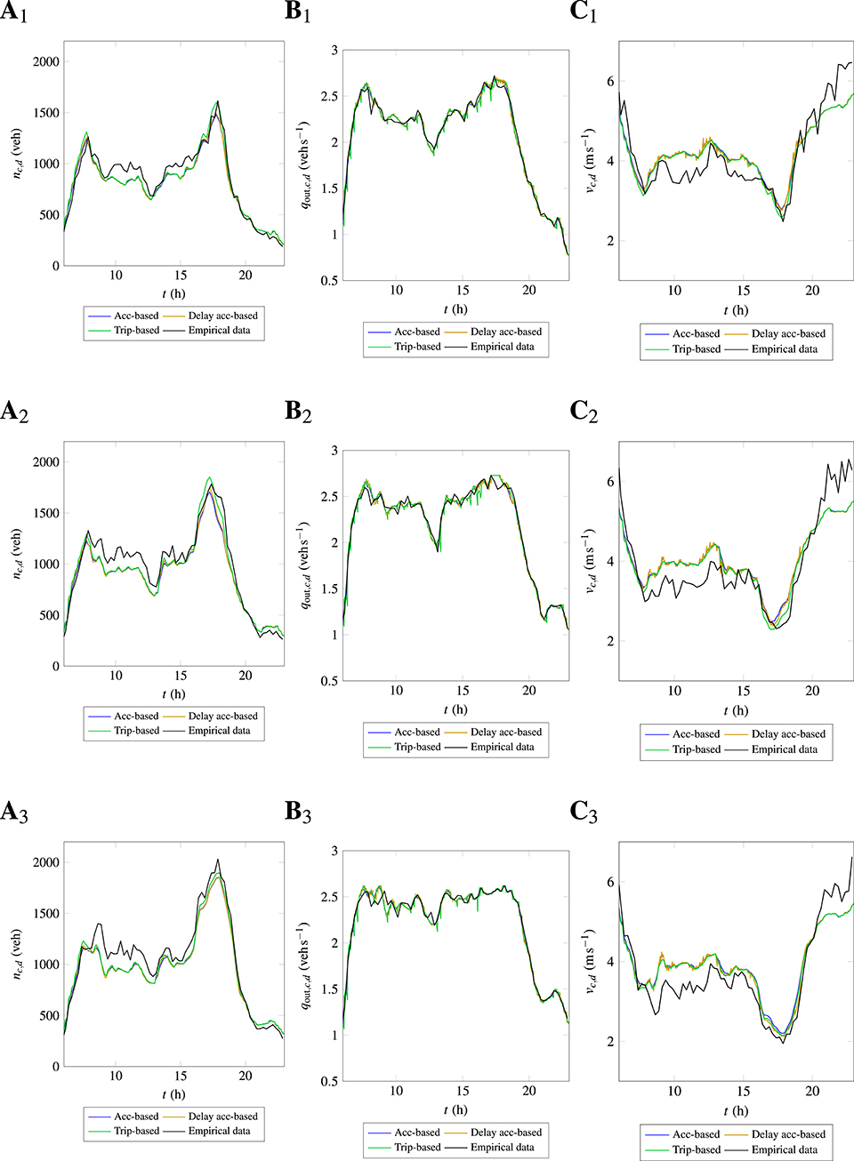
Figure 9. Evolution of accumulation, outflow, and mean speed in the City center using single bi-linear 3D-MFD for 3 weekdays. (A_i) Accumulation, (B_i) outflow, (C_i) mean speed, where i is day.

This phenomenon can be noticed in the case of 2D-MFD as well, where using a single functional fit cannot describe the relationship between travel production and accumulation for the whole range of observed accumulations. Consequently, inconsistencies in the evolution of traffic state variables can be observed for a certain range of accumulations. As in the case of 2D-MFD, this limitation can be addressed using piece-wise bi-linear 3D-MFDs instead of single 3D-MFD. Estimating piece-wise linear or quadratic 2D-MFD is a straight forward whereas, computing a piece-wise bi-linear 3D-MFD is more complicated. At least three different approaches can be proposed here: (i) the range of accumulation of private cars can be divided into several bins and a 3D-MFD fit can be defined within each bin, (ii) the range of accumulations of public transport vehicles can be binned, where different 3D-MFDs can be defined for different bins and (iii) both accumulations of private cars and public transport vehicles can be divided into several bins. The third approach is not feasible using empirical data, as private cars and public transport vehicles tend to operate within a particular region in the accumulation space. Thus, 3D-MFD fits cannot be defined for the ranges of accumulations, where empirical data is not available. However, this approach can be used in micro-simulation studies, where simulations with different demand patterns can be used to cover the entire accumulation space. Either the first or second approach can be used with the current data set.

Another critical factor to consider while defining the functional fit is the scatter in the data. It was already shown the existence of the hysteresis phenomenon in the case of 2D-MFD due to various factors like network heterogeneity, demand pattern (Buisson and Ladier, 2009; Leclercq and Paipuri, 2019). A framework to account for this hysteresis phenomenon in the MFD modeling framework was proposed in Paipuri et al. (2019). This phenomenon can be characterized by two different paths on the accumulation-production plane, one for network loading and another network unloading phases. These paths can be differentiated based on time periods, where the network is in loading or unloading state. Characterization and quantification of the hysteresis phenomenon in the case of 3D-MFD is still an open question. However, the scatter in the present empirical data suggest the differences in network states during loading and unloading phases. Thus, it is relevant to consider different 3D-MFD for different time periods, depending on the state of the network. In other words, the approach proposed in Paipuri et al. (2019) can be extended to the present bi-modal case, where different 3D-MFD fits are considered for network loading and unloading states. As the present empirical data covers a typical 24 h period for each weekday, four different 3D-MFDs are expressed for four different time periods namely, (i) midnight to morning peak, (ii) morning peak to midday, (iii) midday to evening peak and (iv) evening peak to midnight. Therefore, instead of considering piece-wise 3D-MFDs based on accumulation ranges of private cars or public transport vehicles, multi 3D-MFDs are estimated based on the state of network loading for different time periods.

Table 2 presents the coefficients of bi-linear 3D-MFDs for segregated time periods. For each time period, empirical data for all 5 days are gathered and a mean 3D-MFD fit is estimated. Note that the exact cutoff time for each period depends on empirical data under study and the proposed time periods should not be taken as a universal law. The cutoff times should be chosen in such a way to minimize the scatter in empirical 3D-MFD data. Figure 10 shows the evolution of traffic states using the proposed multi 3D-MFD approach in the City center region. Firstly, it is evident that the evolution of accumulations and mean speeds in Figures 10A₁–A₃,C₁–C₃, respectively have a good correspondence with empirical data compared to Figure 9. It can be noticed that the MFD-based models properly predict both peak and off-peak periods. The only significant discrepancy observed is at the morning peak hour for day 2, where simulation results under-predicted the accumulation and over-predicted the mean speed. This can be expected due to the variations in day-to-day 3D-MFD, even within the same time period. However, the simulation results show a satisfactory consistency with empirical data. Therefore, the proposed multi 3D-MFD approach based on the different time periods is justified. An inherent drawback of the multi 3D-MFD or piece-wise 3D-MFD approaches is that the occurrence of discontinuities in the outflow evolution during the transition from one 3D-MFD to another. In the outflow evolution plots shown in Figures 10B₁–B₃, the presence of discontinuities around 08:15 AM can be clearly observed. It is to be noted that these discontinuities occur at other transition times as well, albeit their magnitudes are small. In the proposed multi 3D-MFD approach, discontinuities occur only at the transition time periods whereas, a piece-wise 3D-MFD approach based on the range of accumulations can result in many discontinuities depending on the variability in the accumulation evolution. Moreover, these discontinuities do not have a significant influence on the applications based on MFD-based simulations.

TABLE 2

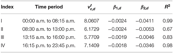
Table 2. Fit parameters of multi bi-linear 3D-MFD fits for City center region.

FIGURE 10

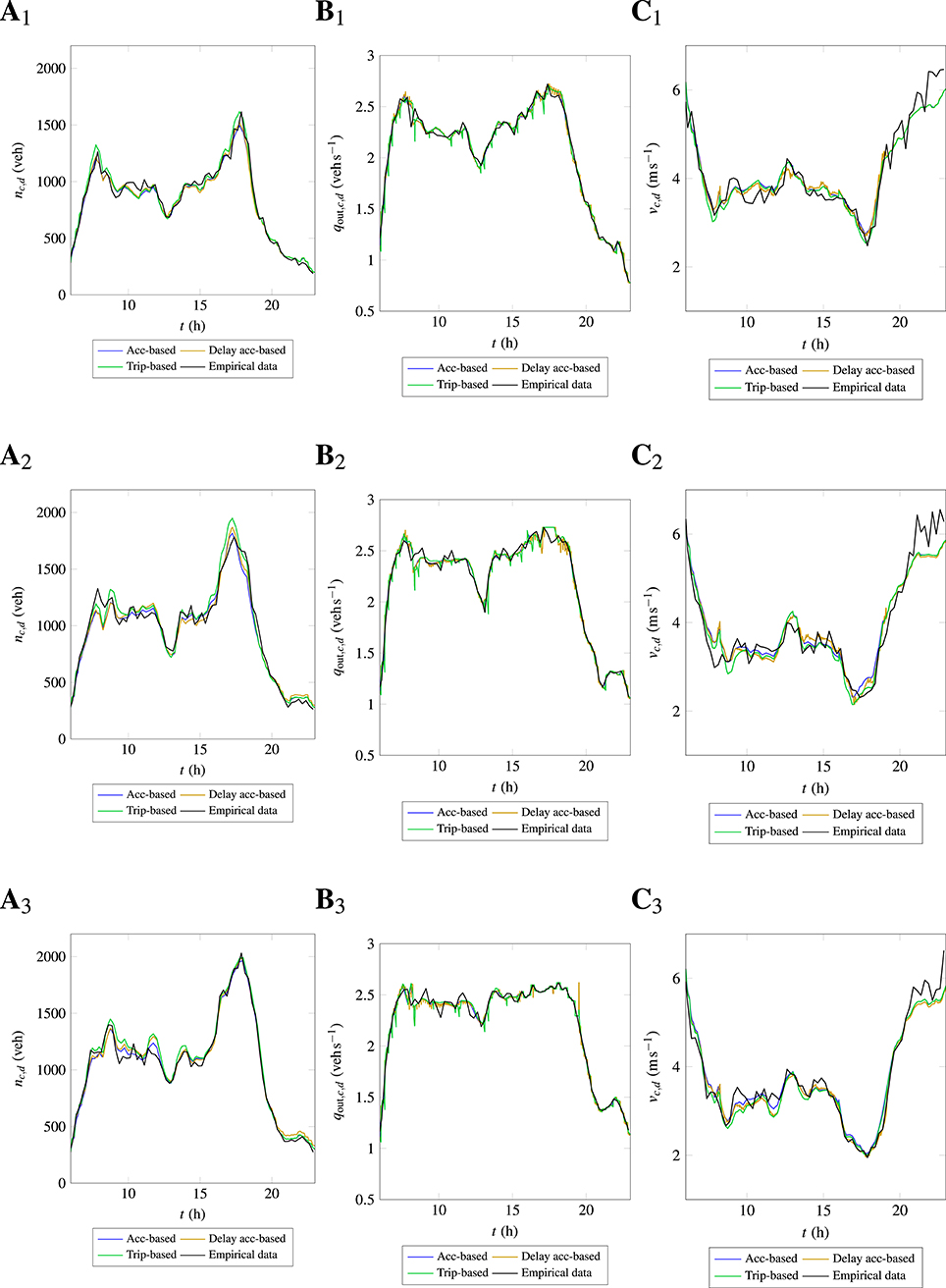
Figure 10. Evolution of accumulation, outflow, and mean speed in the City center using multi bi-linear 3D-MFDs for 3 weekdays. (A_i) Accumulation, (B_i) outflow, (C_i) mean speed, where i is day.

In order to present the differences between different MFD-based models, day 1 is selected. Figure 11 shows the evolution of accumulation and mean speed for day 1 in the City center region. It was showed in Paipuri and Leclercq (2020) that the accumulation-based model is most diffusive and trip-based is least diffusive, whereas the diffusivity of the accumulation-based model with outflow delay lies in-between two of them. This can be observed in the inset plots that show the detailed evolution of traffic states during the morning and evening peak hours. The trip-based model yields the highest peak accumulation and the accumulation-based model gives the lowest peak amongst the considered models. Figure 11B shows the evolution of mean speed, where the discontinuity can be noticed at 08:15 a.m. due to the transition from one 3D-MFD. The inset plots show the mean speed evolution during peak hours and it is again clear that trip-based is closer to empirical data and accumulation-based is most diffusive.

FIGURE 11

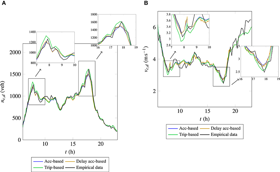
Figure 11. Evolution of accumulation and mean speed in the City center using multi bi-linear 3D-MFDs for day 1. (A) Accumulation, (B) mean speed.

6.2. Wiedikon

A similar approach is used for the Wiedikon region to validate the MFD models with empirical data. Table 3 presents the fit coefficients of multi bi-linear 3D-MFD fits for different time periods. Different cutoff times are defined for the Wiedikon region compared to the City center to segregate the time periods. It is also noticed that omitting the data from 00:00 to 06:00 a.m. for the Wiedikon region results in a stable 3D-MFD fit with less scatter. This can be due to fewer data usually available during the early morning, which can amplify the noise inherent to data. The fit coefficient β_2,r, which quantifies the effect of public transport vehicles on private cars mean speed, is positive for time periods II and III. It signifies that the presence of public transport vehicles is increasing the mean speed of private cars, which is counter-intuitive. However, this coefficient in Table 1, which presents mean 3D-MFD fit for the entire data set, is negative. The reason for the positive coefficient for those two time periods can be a smaller operating range of accumulations of public transport vehicles, which are 2 and 3 veh, respectively. As the number of circulating public transport vehicles is practically the same during these two time periods, quantification of the effect of public transport vehicles on cars is not representative.

TABLE 3

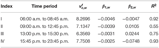
Table 3. Fit parameters of multi bi-linear 3D-MFD fits for Wiedikon region.

Another important observation in empirical data of the Wiedikon region is the traffic states of evening peak hour. It can be noticed from Figure 3 that there is a big difference in the peak accumulations during morning peak and evening peak hours for the Wiedikon region. The maximum number of circulating vehicles during the morning peak period does not exceed 1,000 veh, whereas the evening peak has as many as 2,000 veh. There can be many factors contributing to this asymmetric peak trend like the two-layered perimeter control implemented for the city of Zurich (Ambühl et al., 2018). At the same time, data points in the congestion branch of 3D-MFD can be observed from empirical data that is shown in Figure 2B. Thus, it suggests that there are either internal bottlenecks or congestion spillbacks from outside the Wiedikon region during the evening peak hour that restricts the outflow and increasing the accumulation. In order to reproduce a similar situation, supply restriction is imposed on the MFD-based models from 17:00 p.m. to 19:00 p.m., which is equal to the outflow from empirical data. It is worth noting that without such information to the MFD-based models, it is not possible to obtain a good correspondence between simulation results and empirical data during evening peak hour.

Figure 12 shows the evolution of accumulations, outflow and mean speed of simulation results for the considered 3 weekdays for the Wiedikon region. MFD-based models reproduce the evolution of traffic states during the morning and evening peak hours reasonably well. During morning peak hour, small discrepancies can be noticed in the simulation results. For day 1, MFD simulations over-predict and for other days, they under-predict the peak accumulation. This is again due to the scatter in data, where simulation results follow the mean evolution. In the same way, simulation results either over-predict or under-predict the peak accumulation during evening peak hour too. It is worth noting that 3D-MFD fits are estimated using the data of all 5 weekdays and thus, scatter in the data for the other 2 days can influence the results. A satisfactory coherence is noticed for the off-peak periods in the present case. Overall, the accuracy of the simulation results with respect to empirical data is inferior to the case of the City center region. This can be attributed to more scatter in empirical 3D-MFD for the Wiedikon region compared to the City center.

FIGURE 12

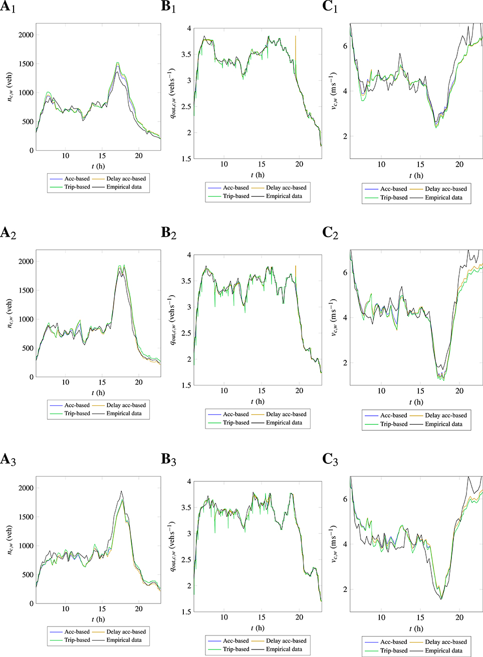
Figure 12. Evolution of accumulation, outflow, and mean speed in the Wiedikon using multi bi-linear 3D-MFDs for 3 weekdays. (A_i) Accumulation, (B_i) outflow, (C_i) mean speed, where i is day.

6.3. City Center Using 2D-MFD

The final part of the current work demonstrates the importance of considering bi-modal MFD in the MFD-based simulations for the networks with an ample number of circulating public transport vehicles. Instead of separating the modes of vehicles, it is assumed that the network consists of a single population of vehicles. The empirical data of private cars and public transport vehicles are treated alike and an MFD is established between total network production and total network accumulation. In other words, this method yields a classical 2D-MFD relating the total accumulation to the total production in the network. This 2D-MFD can be used with regular MFD-based models (Mariotte et al., 2017; Mariotte and Leclercq, 2019) to predict the evolution of accumulation and mean speed. A linear functional form for the mean speed fit is considered, which can be expressed as follows,

$\begin{array}{ll}{v}_d=v_d^f+{\beta }_d{n}_d,& (10)\end{array}$

where $v_d^f$ is free-flow mean speed and n_d is accumulation of vehicles in the City center. In order to be consistent with the 3D-MFD approach, multiple 2D-MFDs based on different time periods are considered in the present context as well. Table 4 presents the fit coefficients for different time periods. As in the previous case, data points from all 5 weekdays are considered within each time period to estimate the fit coefficients.

TABLE 4

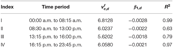
Table 4. Fit parameters of multi linear 2D-MFD fits for City center region.

Figure 13 shows the evolution of accumulation and mean speed for the City center region using multi linear 2D-MFDs for day 1. It is clear from the results that the evolution of both accumulation and mean speed of the MFD-based models are significantly different from empirical data. It is to be noted that the same inflow demand and mean trip lengths used as in the case of 3D-MFD simulation results presented in Figure 11. Thus, it is evident that the difference comes from the estimated MFD fit. Public transport vehicles have a negative marginal effect on cars and 3D-MFD can capture this phenomenon, where the outflow of private cars decreases with increasing accumulation of public transport vehicles. However, in the case of 2D-MFD, this phenomenon is absent and hence, it results in higher outflows, which in-turn yield lower accumulations. From the plots, it is clear that the accumulation evolution is consistently under-predicted by the simulation results. Hence, it can be concluded that using multi-modal MFD is essential in the MFD modeling framework to account for the interactions between different modes in the network.

FIGURE 13

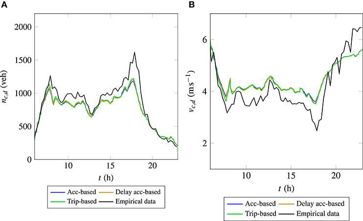
Figure 13. Evolution of accumulation and mean speed in the City center using multi linear 2D-MFDs for day 1. (A) Accumulation, (B) mean speed.

7. Conclusions

The primary objective of this work is to validate the bi-modal MFD-based models using empirical data of the city of Zurich. The data contains the time series values of accumulations and productions for private cars and public transport vehicles for 7 days for two different regions, namely, City center and Wiedikon. However, crucial information about the mean trip lengths, inflow demand or OD matrix is missing to perform a representative MFD simulation.

A single bi-linear functional form is considered to fit the empirical data as the first step toward validation. A simple yet, efficient method to estimate the inflow demand is proposed. Two different approaches can be used in the context of inflow demand estimation. The first approach assumes the travel time to be constant throughout the trip. In contrast, a more accurate second approach accounts for the variability in travel time by discretizing the time by a finite time step. The second approach relies on the finer resolution of the mean speed data. Two approaches yield very similar inflow demand profiles in the present work as the mean speed is aggregated for every 15 min and travel times are typically lower than the aggregation interval. In order to estimate the mean trip lengths, a network exploration technique is used. The whole Zurich network is randomly sampled and the shortest paths between OD pairs are computed. The trips that transverse across the regions under consideration are extracted to estimate the trip lengths distribution and eventually, mean trip lengths.

It is noticed from the simulation results that using a single bi-linear 3D-MFD is a too crude approximation for predicting the evolution of traffic states accurately. Hence, the approach of multi 3D-MFD fits based on certain time periods is proposed. Four different 3D-MFDs are considered covering peak and off-peak periods during morning and evening times. It is noticed that the simulation results with the proposed multi bi-linear 3D-MFDs are relatively in good agreement for both the City center and Wiedikon regions. The improvement from using single 3D-MFD to multi 3D-MFDs in the simulation results can be attributed to a better representation of empirical data. The current framework can be extended to validate the passenger flow instead of the flow of vehicles. Estimating an empirical passenger 3D-MFD is more challenging as the occupancy data of private cars and public transport vehicles is difficult to gather. If the data is available, the current validation method can be used with the accumulation of passengers as the primary unknown variable instead of the accumulation of cars. Finally, the paper is concluded by showing that MFD-based models based on 2D-MFD have limitations, especially when the networks with public transport are considered. The shortcomings are demonstrated by performing an MFD-based simulation using 2D-MFD instead of 3D-MFD.

Data Availability Statement

The data analyzed in this study is subject to the following licenses/restrictions: we access the data on the courtesy of their owner at ETHZ. The data should be asked to the owners. Requests to access these datasets should be directed to Loder Allister, allister.loder@ivt.baug.ethz.ch.

Author Contributions

LL came up with the idea, participated in the discussion of the results, edited the manuscript, and responsible for funding acquisition. MP did the data curation, implemented the models, performed the formal analysis, investigation and visualization of results, and preparation of the manuscript.

Funding

MP and LL acknowledge the funding from the European Research Council (ERC) under the European Union's Horizon 2020 Research and Innovation Program (grant agreement no 646592 – MAGnUM project).

Conflict of Interest

The authors declare that the research was conducted in the absence of any commercial or financial relationships that could be construed as a potential conflict of interest.

The reviewer LA declared a past co-authorship with one of the authors LL to the handling editor.

Acknowledgments

The authors are very grateful to Dr. Allister Loder and all the ETHZ transportation groups lead by Prof. Axhausen and Prof. Menendez for sharing the Zurich city data from their previously published work (Loder et al., 2017). The authors would like thank the reviewers for their insightful comments and suggestions, which improved the quality of the manuscript.

References

Ambühl, L., Loder, A., Menendez, M., and Axhausen, K. (2018). “A case study of Zurich's two-layered perimeter control,” in Proceedings of 7th Transport Research Arena TRA 2018 (Vienna).

Google Scholar

Ampountolas, K., Zheng, N., and Geroliminis, N. (2017). Macroscopic modelling and robust control of bi-modal multi-region urban road networks. Transport. Res. B Methodol. 104, 616–637. doi: 10.1016/j.trb.2017.05.007

CrossRef Full Text | Google Scholar

Arnott, R. (2013). A bathtub model of downtown traffic congestion. J. Urban Econ. 76, 110–121. doi: 10.1016/j.jue.2013.01.001

CrossRef Full Text | Google Scholar

Barmpounakis, E., and Geroliminis, N. (2020). On the new era of urban traffic monitoring with massive drone data: the pNEUMA large-scale field experiment. Transport. Res. C Emerg. Technol. 111, 50–71. doi: 10.1016/j.trc.2019.11.023

CrossRef Full Text | Google Scholar

Batista, S., Leclercq, L., and Geroliminis, N. (2019). Estimation of regional trip length distributions for the calibration of the aggregated network traffic models. Transport. Res. B Methodol. 122, 192–217. doi: 10.1016/j.trb.2019.02.009

CrossRef Full Text | Google Scholar

Batista, S. F. A., Leclercq, L., and Menendez, M. (2020). Regional dynamic traffic assignment framework with time-dependent trip lengths (under preparation).

Boeing, G. (2017). OSMnx: new methods for acquiring, constructing, analyzing, and visualizing complex street networks. Comput. Environ. Urban Syst. 65, 126–139. doi: 10.1016/j.compenvurbsys.2017.05.004

CrossRef Full Text | Google Scholar

Boyac, B., and Geroliminis, N. (2011). Estimation of the network capacity for multimodal urban systems. Proc. Soc. Behav. Sci. 16, 803–813. doi: 10.1016/j.sbspro.2011.04.499

CrossRef Full Text | Google Scholar

Buisson, C., and Ladier, C. (2009). Exploring the impact of homogeneity of traffic measurements on the existence of Macroscopic Fundamental Diagrams. Transport. Res. Rec. J. Transport. Res. Board 2124, 127–136. doi: 10.3141/2124-12

CrossRef Full Text | Google Scholar

Cao, J., and Menendez, M. (2015). System dynamics of urban traffic based on its parking-related-states. Transport. Res. B Methodol. 81, 718–736. doi: 10.1016/j.trb.2015.07.018

CrossRef Full Text | Google Scholar

Chiabaut, N., Xie, X., and Leclercq, L. (2014). Performance analysis for different designs of a multimodal urban arterial. Transportmetr. B Trans. Dyn. 2, 229–245. doi: 10.1080/21680566.2014.939245

CrossRef Full Text | Google Scholar

Daganzo, C. F. (2007). Urban gridlock: macroscopic modeling and mitigation approaches. Transport. Res. B Methodol. 41, 49–62. doi: 10.1016/j.trb.2006.03.001

CrossRef Full Text | Google Scholar

Daganzo, C. F., and Lehe, L. J. (2015). Distance-dependent congestion pricing for downtown zones. Transport. Res. B Methodol. 75, 89–99. doi: 10.1016/j.trb.2015.02.010

CrossRef Full Text | Google Scholar

Friesz, T. L., Luque, J., Tobin, R. L., and Wie, B.-W. (1989). Dynamic network traffic assignment considered as a continuous time optimal control problem. Oper. Res. 37, 893–901. doi: 10.1287/opre.37.6.893

CrossRef Full Text | Google Scholar

Genser, A., and Kouvelas, A. (2020). “Optimum route guidance in multi-region networks: a linear approach,” in Transportation Research Board 99th Annual Meeting Transportation Research Board (Washington, DC).

Google Scholar

Geroliminis, N. (2009). “Dynamics of peak hour and effect of parking for congested cities,” in Transportation Research Board 88th Annual Meeting Transportation Research Board (Washington, DC).

Google Scholar

Geroliminis, N., and Daganzo, C. F. (2008). Existence of urban-scale macroscopic fundamental diagrams: Some experimental findings. Transport. Res. B Methodol. 42, 759–770. doi: 10.1016/j.trb.2008.02.002

CrossRef Full Text | Google Scholar

Geroliminis, N., Zheng, N., and Ampountolas, K. (2014). A three-dimensional macroscopic fundamental diagram for mixed bi-modal urban networks. Transport. Res. C Emerg. Technol. 42, 168–181. doi: 10.1016/j.trc.2014.03.004

CrossRef Full Text | Google Scholar

Godfrey, J. (1969). The mechanism of a road network. Traffic Eng. Control 11, 323–327.

Google Scholar

Gu, Z., Shafiei, S., Liu, Z., and Saberi, M. (2018). Optimal distance- and time-dependent area-based pricing with the network fundamental diagram. Transport. Res C Emerg. Technol. 95, 1–28. doi: 10.1016/j.trc.2018.07.004

CrossRef Full Text | Google Scholar

Haddad, J., and Mirkin, B. (2017). Coordinated distributed adaptive perimeter control for large-scale urban road networks. Transport. Res C Emerg. Technol. 77, 495–515. doi: 10.1016/j.trc.2016.12.002

CrossRef Full Text | Google Scholar

Haddad, J., and Zheng, Z. (2018). Adaptive perimeter control for multi-region accumulation-based models with state delays. Transport. Res B Methodol. 137, 133–153. doi: 10.1016/j.trb.2018.05.019

CrossRef Full Text | Google Scholar

Hagberg, A. A., Schult, D. A., and Swart, P. J. (2008). “Exploring network structure, dynamics, and function using NetworkX,” in Proceedings of the 7th Python in Science Conference (SciPy2008), eds G. Varoquaux, T. Vaught, and J. Millman (Pasadena, CA), 11–15.

Google Scholar

Huang, C., Zheng, N., and Zhang, J. (2019). Investigation of bimodal macroscopic fundamental diagrams in large-scale urban networks: empirical study with GPS data for Shenzhen city. Transport. Res. Rec. 2673, 114–128. doi: 10.1177/0361198119843472

CrossRef Full Text | Google Scholar

Kavianipour, M., Saedi, R., Zockaie, A., and Saberi, M. (2019). Traffic state estimation in heterogeneous networks with stochastic demand and supply: mixed Lagrangian-Eulerian approach. Transport. Res. Rec. 2673, 114–126. doi: 10.1177/0361198119850472

CrossRef Full Text | Google Scholar

Keyvan-Ekbatani, M., Kouvelas, A., Papamichail, I., and Papageorgiou, M. (2012). Exploiting the fundamental diagram of urban networks for feedback-based gating. Transport. Res. B Methodol. 46, 1393–1403. doi: 10.1016/j.trb.2012.06.008

CrossRef Full Text | Google Scholar

Lamotte, R., and Geroliminis, N. (2016). “The morning commute in urban areas: insights from theory and simulation,” in Transportation Research Board 95th Annual Meeting Transportation Research Board (Washington, DC).

Google Scholar

Leclercq, L., and Paipuri, M. (2019). Macroscopic traffic dynamics under fast-varying demand. Transportation Science 53, 1526–1545. doi: 10.1287/trsc.2019.0908

CrossRef Full Text | Google Scholar

Leclercq, L., Sénécat, A., and Mariotte, G. (2017). Dynamic macroscopic simulation of on-street parking search: a trip-based approach. Transport. Res. B Methodol. 101, 268–282. doi: 10.1016/j.trb.2017.04.004

CrossRef Full Text | Google Scholar

Loder, A., Ambühl, L., Menendez, M., and Axhausen, K. W. (2017). Empirics of multi-modal traffic networks-using the 3D macroscopic fundamental diagram. Transport. Res. C Emerg. Technol. 82, 88–101. doi: 10.1016/j.trc.2017.06.009

CrossRef Full Text | Google Scholar

Loder, A., Dakic, I., Bressan, L., Ambühl, L., Bliemer, M. C., Menendez, M., et al. (2019). Capturing network properties with a functional form for the multi-modal macroscopic fundamental diagram. Transport. Res. B Methodol. 129, 1–19. doi: 10.1016/j.trb.2019.09.004

CrossRef Full Text | Google Scholar

Mahmassani, H., Williams, J., and Herman, R. (1984). “Investigation of network-level traffic flow relationships: some simulation results,” in Transportation Research Record, 121–130. Available online at: https://www.scholars.northwestern.edu/en/publications/investigation-of-network-level-traffic-flow-relationships-some-si

Google Scholar

Mariotte, G., and Leclercq, L. (2019). Flow exchanges in multi-reservoir systems with spillbacks. Transport. Res. B Methodol. 122, 327–349. doi: 10.1016/j.trb.2019.02.014

CrossRef Full Text | Google Scholar

Mariotte, G., Leclercq, L., and Laval, J. A. (2017). Macroscopic urban dynamics: analytical and numerical comparisons of existing models. Transport. Res. B Methodol. 101, 245–267. doi: 10.1016/j.trb.2017.04.002

CrossRef Full Text | Google Scholar

Mohajerpoor, R., Saberi, M., Vu, H. L., Garoni, T. M., and Ramezani, M. (2020). H_∞ robust perimeter flow control in urban networks with partial information feedback. Transport. Res. B Methodol. 137, 47–73. doi: 10.1016/j.trb.2019.03.010

CrossRef Full Text | Google Scholar

Ortigosa, J., Zheng, N., Menendez, M., and Geroliminis, N. (2015). “Analysis of the 3D-vMFDs of the urban networks of Zurich and San Francisco,” in 2015 IEEE 18th International Conference on Intelligent Transportation Systems (Las Palmas), 113–118. doi: 10.1109/ITSC.2015.27

CrossRef Full Text | Google Scholar

Paipuri, M., and Leclercq, L. (2020). Bi-modal macroscopic traffic dynamics in a single region. Transport. Res. B Methodol. 133, 257–290. doi: 10.1016/j.trb.2020.01.007

CrossRef Full Text | Google Scholar

Paipuri, M., Leclercq, L., and Krug, J. (2019). Validation of Macroscopic Fundamental Diagrams-based models with microscopic simulations on real networks: importance of production hysteresis and trip lengths estimation. Transport. Res. Rec. 2673, 478–492. doi: 10.1177/0361198119839340

CrossRef Full Text | Google Scholar

Paipuri, M., Xu, Y., González, M. C., and Leclercq, L. (2020). Estimating MFDs, trip lengths and path flow distributions in a multi-region setting using mobile phone data. Transport. Res. Part C: Emerg. Technol. 118:102709. doi: 10.1016/j.trc.2020.102709

CrossRef Full Text | Google Scholar

Ran, B., Boyce, D. E., and LeBlanc, L. J. (1993). A new class of instantaneous dynamic user-optimal traffic assignment models. Oper. Res. 41, 192–202. doi: 10.1287/opre.41.1.192

CrossRef Full Text | Google Scholar

Yildirimoglu, M., and Geroliminis, N. (2014). Approximating dynamic equilibrium conditions with macroscopic fundamental diagrams. Transport. Res. B Methodol. 70, 186–200. doi: 10.1016/j.trb.2014.09.002

CrossRef Full Text | Google Scholar

Yildirimoglu, M., Ramezani, M., and Geroliminis, N. (2015). Equilibrium analysis and route guidance in large-scale networks with MFD dynamics. Transport. Res. C Emerg. Technol. 59, 404–420. doi: 10.1016/j.trc.2015.05.009

CrossRef Full Text | Google Scholar

Zhong, R., Huang, Y., Xiong, J., Zheng, N., Lam, W., and Sumalee, A. (2018). “An optimal control framework for multi-region macroscopic fundamental diagram systems with time delay, considering route choice and departure time choice,” in 21st IEEE International Conference on Intelligent Transportation Systems (Maui, HI), 1962–1967. doi: 10.1109/ITSC.2018.8569905

CrossRef Full Text | Google Scholar