Deep Learning Based Proactive Multi-Objective Eco-Routing Strategies for Connected and Automated Vehicles

1. Introduction

The transportation system in the U.S. produced 28% of the total greenhouse gas (GHG) emissions in 2018, which was the largest share from a single source (EPA, 2020b). Greenhouse gases, CO₂, CH4, and N2O, are the gases that trap heat in the atmosphere (EPA, 2020a). According to the United States Environmental Protection Agency in 2017, 81% of the GHG was CO₂, which is a major contributor to climate change and global warming. Generally, CH4, N2O are converted to “CO₂ equivalent” to estimate GHG emissions (United States Environmental Protection Agency, 2020). In addition, transportation systems contribute to the increase in the produced NOx (Campbell et al., 2018). The air pollutant NOx, which reflects the public health aspect, represents a family of seven compounds, including N2O, which is a greenhouse gas (Cox, 1999). The employment of ICT and connected and automated vehicles (CAVs) has been suggested as a potential solution to alleviate the undesirable social and environmental impact of transportation systems (Zegeye et al., 2009). In particular, routing schemes for CAVs have an explicit impact on traffic (Yang and Recker, 2006; Alfaseeh et al., 2018; Djavadian and Farooq, 2018) and environmental (Tu et al., 2019) characteristics.

Reactive routing uses the current network state, while proactive routing utilizes the predicted state (Bottom, 2000). Proactive routing is considered a promising approach to improve traffic characteristics of a network while avoiding congestion-especially when we employ a high market penetration rate (MPR) of vehicles that are equipped with a routing system that is based on anticipated information (Mahmassani, 1994; Bottom, 2000; Ben-Akiva et al., 2001).

Eco-routing is a special case of routing that specifically considers the environmental aspects (Luo et al., 2016). Several studies in the literature developed reactive eco-routing systems. For instance, Alfaseeh et al. (2019) and Djavadian et al. (2020) developed single as well as multi-objective eco-routing for CAVs and found encouraging results. A developed review paper by Alfaseeh and Farooq (2020) classified eco-routing models and illustrated the strengths and weaknesses of each category. The common limitations were related to the level of resolution of data points, scale of the case study, and number of objectives optimized at once. With reference to proactive routing in general, a limited number of studies in the literature, especially recent ones, has been noticed. For the few proactive routing studies considering only travel time as the routing objective (Bottom, 2000; Ben-Akiva et al., 2001; Pan et al., 2013), the associated limitations were related to the scale of the case study (Kaufman et al., 1991), level of temporal and spatial resolution (Bilali et al., 2019), use of centralized solutions that suffer from scaling issues, and the use of reflective prediction models (Kaufman et al., 1991; Bottom, 2000; Ben-Akiva et al., 2001; Pan et al., 2013). The found proactive routing studies did not employ sophisticated predictive models, which is a major limitation. The forecasted travel time data points were provided by running the traffic simulation in advance (Ben-Akiva et al., 2001; Kim et al., 2016; Bilali et al., 2019) or based on regression models between speed and other traffic variables, such as density (Pan et al., 2013). In most of the studies, the travel time of time step t + i, obtained from the traffic simulation or historical data, was used in time step t for the proactive routing application, where i is the considered prediction interval (Ben-Akiva et al., 2001).

Most of the previous eco-routing studies minimized fuel consumption, which was estimated at the vehicle level (Rakha et al., 2012; Elbery et al., 2016). This means that the characteristics (mass, rolling coefficients, drag coefficient, etc.) of every vehicle should be known for the estimation process (Wang et al., 2019). This can be challenging when a network level optimization is the objective, which is essential for a meaningful decrease in emissions from transportation systems. We are of the view that smart cities technologies, such as sensors, will be adopted quickly in the near future. The three conventional types of sensors are as follows: passive magnetic sensors, pneumatic tube sensors, and inductive loops (Guerrero-Ibáñez et al., 2018). Unlike the conventional sensors, Miovision SmartSense, which is based on 360 cameras, has the ability to process the captured videos to analyze roadside for vehicle detection, traffic counts, and event alerts (Barlow and Kennett, 2019). Downtown Toronto has already installed, in parts of it, the aforementioned type of sensors, Miovision SmartSense. Hence, this study assumes that the required variables for eco-routing at link level, such as speed and GHG emission rate (ER), are provided by sensors in real time. This network-based approach is more practical and easier to scale compared to the vehicle-based estimation approach. While a vehicle-based approach requires the specifications of every vehicle to estimate GHG emissions, a network-based approach estimates GHG emissions based on gathering traffic and environmental indicators for a defined spatial and temporal level of resolution. This work developed proactive multi-objective eco-routing strategies that can be implemented in routing systems for connected and automated vehicles. Similarly to the proposed reactive routing schemes in Djavadian et al. (2020), a microscopic level of aggregation, an urban network as a case study, and a high level of spatial (link level) and temporal (1 min) resolution were employed in this study. Unlike the previous proactive approaches that were centralized solutions, this study developed the proactive routing strategies based on a dynamic distributed routing control framework, End-to-End Routing for Connected and Automated Vehicles (E2ECAV) (Farooq and Djavadian, 2019). It has been found that distributed routing systems, which adopt different types of communication and several controlling nodes, outperformed the centralized routing systems, which depend on one central node. Centralized routing systems are associated with limitations related to the large investment required, sensitivity to system failure, and complexity in the case of system upgrades (Yang and Recker, 2006). In this study, three eco-routing strategies were applied to optimize travel time (TT), GHG, as well as the combination of TT and GHG. The considered performance indicators for comparison between the different routing strategies were average TT, average VKT, total produced GHG, and total produced NOx emissions. The main contributions of this research work are as follows:

• Examination of the most representative GHG costing approach at highly disaggregate spatial and temporal resolution-the unit of space being a road link and time being 1 min.

• Development of proactive multi-objective eco-routing strategies, while employing the developed prediction model for speed in this study and the developed GHG prediction model in Alfaseeh et al. (2020).

• Detailed comparison between reactive and proactive routing strategies.

In section 2, a brief literature review related to the existing eco-routing studies, their strengths, and weaknesses is presented. In addition, existing predictive models of travel time and GHG and proactive routing studies are illustrated. The specifications of the deployed case study are in section 3. Section 4 includes the details related to the traffic and emission models, GHG costing approaches, and GHG and speed predictive models. Section 5 incorporates the related results and discussion. Finally, section 6 summarizes the major findings and future outlook.

2. Background

Due to the advancements in sensing and communication technologies, their utilization in transportation systems, and the emergence of CAVs, the availability of the real-time high-resolution data has become feasible on a large scale. Such data are adopted to develop highly accurate prediction models that have the potential to be used for proactive routing with multiple objectives. In this section, the studies found in the literature related to the reactive eco-routing, predictive models of travel time and GHG, and proactive routing are briefly presented.

Alfaseeh and Farooq (2020) developed a comprehensive review of eco-routing studies. They reported that the previous reactive eco-routing studies have predominantly used macroscopic level traffic and emission models, were based on small case studies, used centralized routing mechanisms, and have optimized single routing objectives at a time. To overcome the aforementioned limitations, Alfaseeh et al. (2019) applied multi-objective eco-routing in a distributed routing framework. The authors used the per lane weighted average for the GHG cost on links. Although normalizing by the number of lanes resulted in underestimation for the links with a large number of lanes, reductions in the travel time and produced emissions were noticed when multi-objective routing was applied. Djavadian et al. (2020) developed reactive multi-objective eco-routing strategies for CAVs, considering the cost of idling as a penalty at the downstream intersection of a link at every interval. The authors used the marginal cost for GHG in the objective function. They found that including the penalty cost contributed to reductions of 4 and 3% in the average TT and produced total GHG, respectively, in the case of multi-objective routing when compared to single objective routing.

Predictive models are an essential component of the proactive routing application. Vlahogianni et al. (2014) conducted a comprehensive review related to the short-term traffic forecasting. It was noticed that studies mainly considered freeways as their case studies, statistical models, and a temporal resolution of 5 min in most of the cases (Vlahogianni et al., 2014). Freeways were utilized due to the complexity associated with urban congested networks. The vehicular dynamics in urban areas are subject to changes during a short time period (seconds). It is the result of the stop and go phenomena and shorter length of the links when compared to freeways. A low level of temporal resolution was employed due to the scarcity of microscopic data points and the required high computational power. The statistical models, such as the autoregressive integrated moving average (ARIMA) model, are easy to use but may not be able to capture complex non-linear relationship between the variables (Zhang, 2003).

When it comes to travel time prediction, there are two main streams: one that predicts travel time directly and one that predicts speed and consequently travel time. For directly forecasting travel time, several predictive models have been employed. Linear modeling (Zhang and Rice, 2003), nonlinear autoregressive with external inputs (NARX) model (Mane and Pulugurtha, 2018), nonlinear autoregressive model (NAR) (Mane and Pulugurtha, 2018), neural networks (NNs) (Mane and Pulugurtha, 2018), and deep neural networks (Duan et al., 2016; Ran et al., 2019). On the other hand, a large body of literature exists where travel time was implicitly predicted from speed, including Ma et al. (2015), Yao et al. (2017), and Gu et al. (2019). The common features between most of the aforementioned predictive models were the employed low temporal resolution and small case study. The statistical models were also dominating despite their inability to capture the complicated relationship between the variables in concern. Even when a large network was employed as in Zhang et al. (2019), the speed was predicted at a low level of temporal resolution. With regards to the predictive models for speed and travel time, it was found in the literature that long short-term memory (LSTM) outperformed other predictive approaches, including the ARIMA model (Ma et al., 2015).

Related to GHG predictive models, GHG emissions were predicted based on yearly data points of fuel (Zhao et al., 2011), gross domestic product, or other economic factors (Pao and Tsai, 2011; Ameyaw et al., 2019). The predictive models varied from statistical (Tudor, 2016; Rahman and Hasan, 2017) to deep neural networks based (Ameyaw et al., 2019). To overcome the limitations of the previous predictive models, the low spatial (national) and temporal (year) resolution, Alfaseeh et al. (2020) developed a predictive model based on LSTM. The GHG emission rate (ER) at a link level and 1 min time resolution was predicted based on the most representative traffic indicators of the previous time intervals.

With reference to the proactive routing, several frameworks were proposed to minimize travel time (Mahmassani, 1994; Bottom, 2000; Ben-Akiva et al., 2001; Pan et al., 2013; Liang and Wakahara, 2014; Claes, 2015; Liu and Qu, 2016). Bottom (2000) developed a framework for proactive routing in a network with only a single Origin-Destination (OD) pair, 14 links, and 11 OD paths. In terms of the predicted traffic variables, the real-time traffic characteristics and other related data were forecasted at the short and medium term for the proactive routing. The variable message signs (VMS) were employed to provide vehicles with the best route. When the best route was defined, the driver's compliance was not guaranteed. The author thus incorporated a logit model to define the drivers' path choice (Bottom, 2000). Ben-Akiva et al. (2001) proposed DynaMIT, which can be employed to generate real-time guidance to the drivers. Off-line and real time information were adopted. The off-line data as well as historical network conditions were used for the state estimation. While the real-time data were obtained from the control system. Two simulation tools were used: demand and supply. The demand simulator estimated and forecasted the OD flow, departure time of drivers, mode, and route choice. While the supply simulator directly simulated the interactions between the demand and supply (network). Proactive routing was applied while travel time minimization was the routing objective. The predicted travel time was a function of experienced travel time from the previous iteration. Speed on links was estimated based on the linear relationship with density on links in concern. The VMS were used to inform drivers with the information of the best route. With regards to the findings, the authors found that proactive routing was promising, as it contributed to reductions in travel time of vehicles (Ben-Akiva et al., 2001). Pan et al. (2013) suggested proactive re-routing strategies to reduce travel time. The authors predicted congestion based on density/jam density ratio. The speed was predicted based on the Greenshield model, the linear relationship between density and speed, which is a limitation as realistically the relationship is not linear. When the density is low, the speed is underestimated (Papacostas and Prevedouros, 1993). The authors found that their rerouting performed as good as the dynamic traffic assignment (Pan et al., 2013). Another example is the work by Liang and Wakahara (2014), who applied re-routing based on congestion prediction. One of the developed predictive models was based on the spatiotemporal correlation. The authors assumed that the traffic flow was constant during each prediction time interval, which is unrealistic. Liu and Qu (2016) proposed a dynamic congestion model based on crowdsourcing in order to apply proactive routing for a set of cooperative vehicles by predicting the probability distribution of traffic conditions. The adopted time interval for the routes update was 1 min, and the data were obtained from the GPS traces and social media. They found that their approach outperformed the reactive routing approach (Liu and Qu, 2016).

To summarize, the existing predictive models are associated with limitations related to the spatial and temporal resolution. The proactive routing studies did not adopt efficient and accurate predictive models and were used in the context of a centralized routing framework. The centralized routing frameworks require a large infrastructure investment, are highly sensitivity to system failures, and involve high degree of complexity in the case of a system upgrade (Farooq and Djavadian, 2019). This study therefore tackled the aforementioned limitations. To the best of our knowledge, our study is the first of its kind to apply the proactive multi-objective eco-routing while deploying deep learning based predictive models in a distributed routing framework.

3. Case Study

Downtown Toronto's road network was adopted as a case study because it experiences high levels of recurrent congestion-especially during the morning peak period (Council of Ministers Transportation and Highway Safety, 2012). Downtown Toronto is the financial center of Canada and has the highest job density among the major cities in the country. The network is composed of 223 links (road segments between two intersections) and 76 intersections. Based on the 2019/2020 Toronto's vital report (Toronto Foundation, 2020), several factors contribute to the excessive congestion levels in Toronto. The population of Toronto has increased yearly by 1% since 2011. Due to high cost of living, Toronto is the most expensive major city in the country. The ownership costs are growing four times faster than income, while renting costs have grown two times faster than income over the last decade (Toronto Foundation, 2020).

The vehicular demand was provided by the Transportation Tomorrow Survey (TTS) for the period between 7:45 a.m. and 8:00 a.m. for the year 2014 (DMG, 2011). Additionally, the OD of the demand was provided by TTS. Links in the case study are associated with different features with respect to the speed limit, number of lanes, and number of directions. That is, a high level of heterogeneity is assured for a generic application. Figure 1 illustrates the area including the major roads. Links of speed limits of 40 and 60 km/h represent 30 and 59%, respectively, of links in the case study. Links of speed limits of 10, 30, and 80 km/h represent 2, 1, and 8%, respectively, of links in the case study. With regards to the number of lanes, 1, 2, 3, and 4 of 7, 71, 15, and 7%, respectively, are used.

FIGURE 1

Figure 1. Case study, Downtown Toronto.

4. Methodology

This section includes the specifications of the employed traffic and emission models, investigated GHG costing approaches, adopted GHG and speed predictive models, and the routing strategies considered. Figure 2 demonstrates the followed general framework in this study. The estimated second-by-second speed and acceleration were used for calculating GHG emissions. Then five GHG costing approaches, which considered different levels of spatial and temporal resolution, were investigated. After defining the best GHG costing approach, single- and multi-objective reactive and proactive routing strategies were applied. Finally, a comprehensive comparison has been conducted to illustrate the impact of routing vehicles proactively.

FIGURE 2

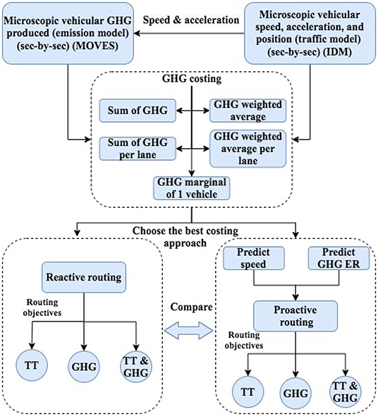
Figure 2. Methodology followed in this study.

4.1. Traffic and Emission Models

Microscopic traffic (Djavadian and Farooq, 2018) and emission (USEPA, 2015) simulators were deployed in this study to obtain high resolution data points at every second. The Intelligent Driver Model (IDM) (Treiber et al., 2000) was the adopted car-following model for the displacement estimation at every second, which was used to calculate the speed of vehicles (Djavadian and Farooq, 2018). Motor Vehicle Emission Simulator (MOVES) was the employed emission model to estimate the second-by-second GHG (in CO_2eq) of every vehicle (USEPA, 2015). The produced second-by-second emissions by vehicles were estimated based on the vehicle operating mode, which depends on the vehicle-specific power (USEPA, 2015). According to the 2012 Canada-United States Air Quality Agreement Progress Report (International Joint Commission, 2012), Canada started using MOVES the summer of 2012. The second-by-second traffic and environmental variables were captured and then used to estimate the space mean link indicators, such as speed (km/hour), density (veh/km), flow (veh/hour), and GHG ER (gram), while considering the suitable spatial and temporal intervals. When all of the vehicles reached their destinations, the simulation ended. The indicators of links, speed, density, GHG, and flow were updated at every minute. As links in an urban road network are shorter and there are very few overtaking/lane changing opportunities in a congested network, our lateral movement model assigns the lane to a vehicle only at the beginning of the link. It is also worth mentioning that First-In-First-Out (FIFO) logic at intersections was deployed. The aforementioned two assumptions related to the lateral movement and logic at intersections do not affect the comparative analysis between the different routing strategies developed. This is stemmed from the fact that the aim in this paper was to investigate the impact of different routing strategies rather than different controlling techniques at intersections.

4.2. GHG Costing Approaches

Most of the previous studies estimated GHG emissions based on fuel consumption, which requires the specifications of every vehicle for high resolution outcome (Wang et al., 2019). Nevertheless, for network scale deployment, there is a need to estimate GHG emissions based on collected data points (speed, GHG ER, etc.) from sensors, which is what we aimed to achieve. This network-based approach is more practical and scalable compared to the vehicle-fuel based approaches. For a robust eco-routing strategy, five different GHG costing approaches have been assessed as illustrated in Table 1. The findings of this analysis can be a guide for practitioners to choose the most suitable GHG costing approach for their setting with respect to the required level of resolution, computational power, and data availability. GHG_cost1(l,Δj), as in Equation (1), is for when GHG cost is the sum of GHG emissions of vehicles N on a studied link l during and interval Δ_j. λ_{(i, l, k)} is a binary variable: 1 if vehicle i is on the studied link l at time k and 0 otherwise. As links in the network have different number of lanes, GHG_cost2(l,Δj) normalizes the total GHG cost based on the number of lanes Z_l following Equation (2). Considering a higher temporal resolution is illustrated in the GHG_cost3(l,Δj) costing approach. The weighted average of produced GHG on link l is the outcome of Equation (3). At every second k of any interval (1–60 s), a weight k, is multiplied by the produced GHG by vehicles. It means that the GHG emissions produced at k = 1 are multiplied by a weight of 1, while the produced GHG emission at second k = 60 is multiplied by a weight of 60. The most recent seconds of an interval Δ_j are associated with a higher weight in the link cost. The sum is then divided by the sum of weights. This costing approach takes the GHG cost at every second, which means it is associated with a high temporal resolution compared to GHG_cost1(l,Δj) and GHG_cost2(l,Δj). GHG_cost4(l,Δj) (Alfaseeh et al., 2019), as in Equation (4), follows the same logic of GHG_cost3(l,Δj) but divides by the number of lanes Z_l of link l to normalize. Finally, GHG_cost5(l,Δj) (Djavadian et al., 2020) is the marginal cost of one vehicle traversing a studied link l. The marginal cost, as shown in Equation (5), depends on an estimated emission rate (ER) and the TT of interval Δ_j on link l. TT is obtained following Equation (6), where D_l represents link l length and V(l, Δ_j) is link l speed of Δ_j time interval.

$\begin{array}{ll}GH{G}_{cost1(l,{\Delta }_j)}={\displaystyle \sum _{k=1}^{{\Delta }_j}}{\displaystyle \sum _{i=1}^N}{\lambda }_{(i,l,k)}\times GH{G}_{(i,k)}& (1)\end{array}$

$\begin{array}{ll}GH{G}_{cost2(l,{\Delta }_j)}=\frac{{\displaystyle {\sum }_{k=1}^{{\Delta }_j}}({\displaystyle {\sum }_{i=1}^N}{\lambda }_{(i,l,k)}\times GH{G}_{(i,k)})}{Z_l}& (2)\end{array}$

$\begin{array}{ll}GH{G}_{cost3(l,{\Delta }_j)}=\frac{{\displaystyle {\sum }_{k=1}^{{\Delta }_j}}(k\times {\displaystyle {\sum }_{i=1}^N}{\lambda }_{(i,l,k)}\times GH{G}_{(i,k)})}{{\displaystyle {\sum }_{k=1}^{{\Delta }_j}}k}& (3)\end{array}$

$\begin{array}{ll}GH{G}_{cost4(l,{\Delta }_j)}=\frac{{\displaystyle {\sum }_{k=1}^{{\Delta }_j}}(k\times \frac{{\displaystyle {\sum }_{i=1}^N}{\lambda }_{(i,l,k)}\times GH{G}_{(i,k)}}{Z_l})}{{\displaystyle {\sum }_{k=1}^{{\Delta }_j}}k}& (4)\end{array}$

$\begin{array}{ll}GH{G}_{cost5(l,{\Delta }_j)}=GH{G}_{ER(l,{\Delta }_j)}\times T{T}_{(l,{\Delta }_j)}& (5)\end{array}$

$\begin{array}{ll}T{T}_{(l,{\Delta }_j)}=\frac{D_l}{V(l,{\Delta }_j)}& (6)\end{array}$

TABLE 1

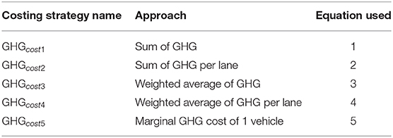
Table 1. GHG costing strategies investigated.

4.3. GHG Emission Rate and Speed Predictive Models

Two separate LSTM networks have been trained to predict the required variables, TT and GHG, for the proactive single and multi-objective routing strategies. The details of the data collection process, including the size of training and testing sets and statistical analysis of the data points are presented in Appendix A. Recurrent neural network (RNN) represent a type of deep neural networks (DNNs). Unlike the artificial neural network (ANN), RNN consists of multiple layers between the input and output layers. The RNN has the capability to specify the correct mathematical manipulation to give an output from an input, whether the relationship between variables is linear or non-linear (Aggarwal, 2018). RNNs introduce the concept of memory. The Long Short-Term Memory (LSTM) network is a category of the RNNs that overcomes the major limitation of regular RNNs, namely the vanishing gradient problem (Amarpuri et al., 2019). LSTM also outperforms the statistical models for time series data, such as ARIMA (Alfaseeh et al., 2020). The LSTM network has been considered as one of the most powerful RNN architectures in the case of sequential data (Lipton et al., 2015). This justifies why LSTM was utilized in this study for prediction. With reference to the LSTM architecture and hyper-parameters, it has been found that the selection of predictors, number of sequences, and the set of hyper-parameters (Hutter et al., 2015; Reimers and Gurevych, 2017) have an explicit impact on the prediction performance. In addition, increasing the depth of the NNs may also introduce further enhancements (Hermans and Schrauwen, 2013; Pascanu et al., 2013). Not to forget that the efficiency of the hyper-parameters tuning process is profound (Snoek et al., 2012). In this study, a comprehensive correlation analysis has been conducted for GHG ER and speed as discussed in Appendix B. For each of the predicted variables, GHG ER and speed, the most representative predictors and number of previous time steps (sequences) used in the models were defined based on the correlation analysis. Then hyper-parameters were tuned in two stages. The manual tuning mainly tried to narrow the search range of the hyper-parameters in concern for a more efficient systematic tuning process based on the Bayesian optimization (Wu et al., 2019). Further details related to the predictive LSTM network can be found in Alfaseeh et al. (2020). To compare the trained LSTM networks, four indicators were utilized: (1) correlation coefficient between observed and predicted GHG ERs (in CO_2eq g/sec), (2) fit to the ideal 45^o line, (3) root mean square error (RMSE), and (4) R².

4.4. Distributed Routing Framework

A dynamic distributed routing framework, E2ECAV proposed by Farooq and Djavadian (2019), was used to test the routing strategies. E2ECAV is based on a network of Intelligent Intersections (I2s) that can dynamically route CAVs. The system guarantees routing in a finite amount of time. When a CAV arrives at any intersection, the CAV declares its destination to the I2, which based on the routing objective/strategy, routes the vehicle in the right direction. It is worth mentioning that for this particular case study, the links cost, whether it was TT or GHG, was updated at every minute. However, E2ECAV can operate on any other update interval. For further description of the E2ECAV, dynamic distributed routing system, and various applications we refer readers to Alfaseeh et al. (2018), Djavadian and Farooq (2018), Farooq and Djavadian (2019), Tu et al. (2019), and Djavadian et al. (2020).

4.5. Routing Strategies

Three strategies based on optimizing TT, GHG, and TT&GHG were examined for each of the reactive and proactive routing schemes, while using simulation. Equation (7) presents the general formula based on the routing objective, TT, GHG, or TT&GHG, where T_i is travel time on link i and E_i is emissions on link i, which is the GHG (in CO_2eq) in our case; n is the number of links of a path k; and W_t and W_e are the weights associated with travel time and emissions, respectively. T and E in Equation (7) are of different units. When multi-objective routing was applied, converting them to a consistent unit (monetary value) was the solution for a realistic application. The adopted TT monetary value was $27.36/hour (Statistics Canada, 2018). The used monetary value of GHG emission was $15.77/Ton (The World Bank, 2019). The weights in Equation (7) were used for the aforementioned normalization process. Every routing strategy was run for five replications of different seeds to account for stochasticity. When the routing strategy was reactive, optimized variables were taken at the current time step. While when the routing strategy was proactive, predicted values of the future time step of the developed predicted models were employed. For instance, routing strategy TT_m means that TT was obtained based on the current time step value of speed following Equation (6). While TT&GHG_a was the proactive routing strategy of when the predicted TT and GHG of the future time step (of the best trained LSTM networks) were utilized. The TT cost of links at every minute followed Equation (6). The link GHG cost in this study was chosen based on the analysis in section 5.1.1 of the different GHG costing approaches.

$\begin{array}{ll}min{\displaystyle \{{\displaystyle \sum _{i=1}^n}{W}_t.T_i+{\displaystyle \sum _{i=1}^n}{W}_e.E_i\}}& (7)\end{array}$

Subject to:

W_t > 0, T_i > 0, W_e > 0, and E_i > 0.

5. Results and Discussion

To apply proactive routing in this study, predictive models were developed. The LSTM based predictive model of the GHG cost was developed in Alfaseeh et al. (2020), but the major findings are shared in section 5.1. The developed speed predictive model is presented in section 5.1. The comparison between the routing strategies are conducted in sections 5.2–5.4.

5.1. Development of the Predictive Models

Before developing the predictive models, the most representative GHG costing approach was investigated, as demonstrated in section 5.1.1. A comprehensive correlation analysis was applied for the GHG ER and speed as illustrated in Appendix B. The developed predictive models are demonstrated in section 5.1.2.

5.1.1. GHG Costing Approaches

This analysis was applied for GHG_m, as reactive routing was the base case, to illustrate which GHG costing approach was the most suitable for our application. Figure 3 shows that normalizing based on the number of lanes as in GHG_cost2 and GHG_cost4 was associated with a slight enhancement in terms of all the performance indicators compared to GHG_cost1 and GHG_cost3, respectively. This is due to the different number of lanes of the links in the network that made the total GHG not reflective of the actual conditions. For the costing approaches GHG_cost1 and GHG_cost3, if the GHG cost of link a with two lanes and b with four lanes are 70 and 100 g, respectively, link a would be prioritized. However, dividing by the number of lanes shows that link b should be prioritized based on GHG_cost2 or GHG_cost4. A reduction in the average TT of around 3% in both GHG_cost2 and GHG_cost4 compared to GHG_cost1 and GHG_cost3, respectively, was observed. Using the total GHG on links of the GHG_cost1 costing approach, triggered the highest average TT, average VKT, total GHG, and total NOx of 16 min, 2 km, 2,518 kg, and 0.716 kg, respectively. The explanation was related to not considering any of the traffic characteristics on the link, such as speed, density, or flow. In the case of GHG_cost1 costing approach, 100 g of the total GHG emission can be for two dramatically different sets of traffic characteristics. The first condition can be for a very congested short link of low capacity, while the other condition can be for an uncongested long link of high capacity.

FIGURE 3

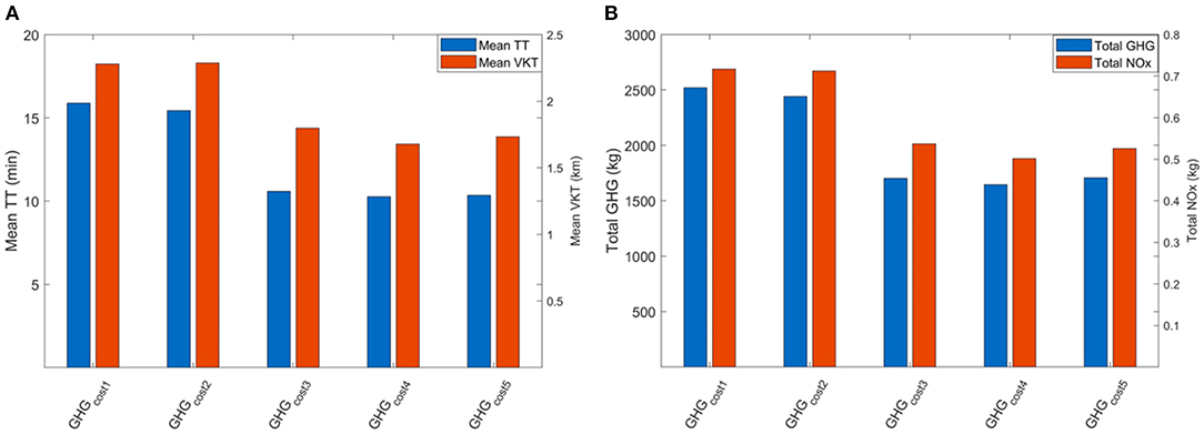
Figure 3. The Impact of Different GHG Costing Approaches on the (A) mean TT and VKT and (B) total GHG and NOx.

GHG_cost3 was associated with significant reductions in the average TT, average VKT, total GHG, and total NOx of 33, 21, 32, and 25%, respectively, when compared to GHG_cost1 as shown in Figure 3. The main justification is the adopted high temporal resolution, compared to GHG_cost1. Furthermore, giving higher weights to the most recent seconds contributed to the improvements in terms of average TT, average VKT total GHG, and total NOx. The closer to the prediction update, the higher the weight for the produced GHG by vehicles. GHG_cost5, which is the marginal cost of one vehicle based on the GHG ER and TT on the studied link, was very much comparable to the GHG_cost4 in terms of the performance. Despite the lower temporal resolution utilized by GHG_cost5 (1 min) compared to GHG_cost4 (1 s), considering TT on studied links by the former contributed to the similar performance (mean TT, mean VKT, total GHG, and total NOx) compared to latter. GHG_cost5 is the most representative and suitable costing approach as it is based on the reflective ER and speed on the studied link as illustrated in Equation (5). Due to the quasi-convex relationship between the speed and GHG ER (Djavadian et al., 2020), too low or too high speed would trigger higher emission rates. Links with too high speed are associated with high GHG ERs but less travel time. Links with too low speed contribute adversely not only to the GHG ER but also to the travel time on the links. It is expected that the GHG marginal cost searches for the optimal combination of speed, VKT, and GHG ER to satisfy the optimization Equation (7). GHG_cost5 was the used costing approach for the related reactive and proactive routing strategies in this study.

5.1.2. GHG and Speed Predictive Models

For each of the predicted variables, GHG ER and speed, a comprehensive list of predictors and number of sequences has been examined. The best predictive LSTM networks of both the GHG ER and speed were of two hidden layers while the hyper-parameters were systematically tuned. In terms of the predictors for GHG ER forecasting (Alfaseeh et al., 2020), the best set was of three sequences of speed, GHG ER, density, and in-links speed. These are the top four highly correlated variables with GHG ER at the 6th min as illustrated in Figure B1. For speed prediction, the best setting was associated with three sequences of speed, density, and in-links speed as demonstrated in Figure B2. In terms of the hyper-parameters, two solvers were considered, the adaptive moment estimation (Adam) methods (Kingma and Ba, 2014) and the stochastic gradient descent with momentum (sgdm) (Robert, 2014). Several hyper-parameters were considered for tuning: initial learning rate, max epochs, learning rate drop factor, momentum, learning rate drop period, number of hidden units of the first LSTM (hidden) layer, and the number of hidden units of the second (LSTM) layer when required. The first stage of tuning was manual, which was adopted to narrow the search range of the optimal hyper-parameters. The next stage was systematic using the Bayesian optimization (Wu et al., 2019; Alfaseeh et al., 2020), which employed the narrowed search range of the manual tuning stage. The training results of the best LSTM predictive networks of the GHG ER and speed are shown in Figures 4A,B, respectively. The figures represent the true/simulated vs. predicted GHG ERs (in CO_2eq g/sec).

FIGURE 4

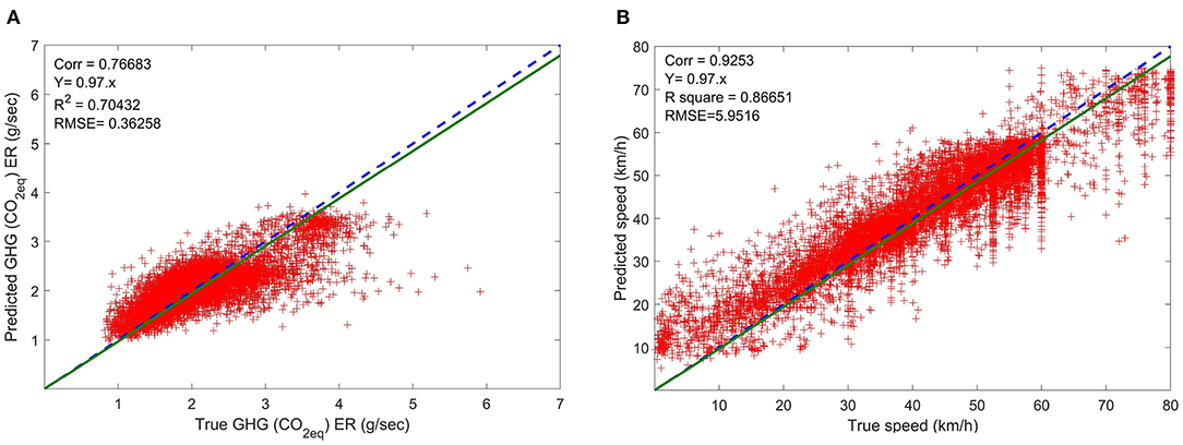
Figure 4. True vs. predicted of the best LSTM models of (A) GHG ERs (in CO_2eq g/sec) (Alfaseeh et al., 2020) and (B) speed.

For the prediction performance, four indicators were deployed: (1) the correlation coefficient between observed and predicted GHG ERs (in CO_2eq g/sec), (2) the fit to the ideal straight curve reflecting on the precision, (3) R² statistics, and (4) the RMSE reflecting on the accuracy (Alfaseeh et al., 2020). The correlation coefficients of GHG ER and speed prediction were 0.77 and 0.92, respectively. The RMSE of the GHG ER and speed predictive models was 0.36 g and 5.95 km/h, respectively. The performance of the speed predictive model was noticeably better than the one of the GHG ER. This is due to the complicated relationship between the GHG ER and the predictors, while speed has more straight forward relationships with the used predictors. For instance, speed and density have a monotonically decreasing relationship (Papacostas and Prevedouros, 1993), while the GHG ER has a quasi-convex relationship with the most important predictor (speed) (Djavadian et al., 2020). It is crucial to note that the developed LSTM predictive models are generally suitable for urban networks. This has been demonstrated in the statistical analysis of traffic and environmental predictors. In the training dataset, speed ranged from 0 to 80 km/h, density ranged from 0 to 150 veh/km/ln, flow ranged from 0 to 8,000 veh/h, and GHG ER ranged from around 0.9 to 5 g/sec. Thus, any urban network of indicators within the aforementioned ranges can be used for prediction purposes.

It is noticed in both Figure 4A and Figure 4B that true values higher than 4 g/sec and 60 km/h, respectively, were not predicted with a high level of accuracy. This stems from the fact that the frequency of the data points reflecting these conditions was much less compared to the other conditions as in Figure A1. The data points reflecting on the GHG ER >4 g/sec, as in Figure A1D, is only 0.007% of the total GHG ER data points. The high GHG is associated with either low or high speed, which is due to the quasi-convex relationship of GHG ER with speed (Djavadian et al., 2020). Similarly, the data points of speed higher than 60 km/h and <20 km/h represent only 0.11% of the total data points, while the data points of speed between 20 and 60 km/h represent 0.89% as in Figure A1A.

5.2. Routing Strategies Analysis

Three strategies that optimized TT, GHG, and TT&GHG were examined for each of the reactive and proactive routing, while using the E2ECAV (Farooq and Djavadian, 2019) routing framework. Single and multi-objectives were considered for reactive and proactive routing. Mean TT, mean VKT, total GHG, and total NOx were the performance indicators taken into account and the results are shown in Figure 5. It is of high importance to include the NOx as a performance factor to assess the impact of the different routing strategies on the public health aspect (Alfaseeh and Farooq, 2020). It is crucial to note that logical constraints have been included for a realistic application while estimating the cost on links. When either the predicted GHG ER or speed of a future time step was negative, the value was set to zero. Predicted speed of a future time step that surpassed the link speed limit was set to the link speed limit. With regards to the results, Figure 5 illustrates that the proactive routing strategies outperformed the reactive ones regardless of the routing objective. The justification of this outcome is threefold. Firstly, the reflective costing approach of the GHG emissions (when GHG was part of the optimization process) was adopted. GHG costing approach optimized not only the GHG ER but also the travel time implicitly to avoid re-routing. The marginal cost prioritized the links of speed close to the optimal value based on the quasi-convex relationship between the GHG ER and speed (Djavadian et al., 2020). Secondly, the sophisticated developed predictive models based on high resolution data points were deployed. Lastly, by taking into account the traffic conditions and their evolution, routing was more proactive than simply being reactive to the current conditions.

FIGURE 5

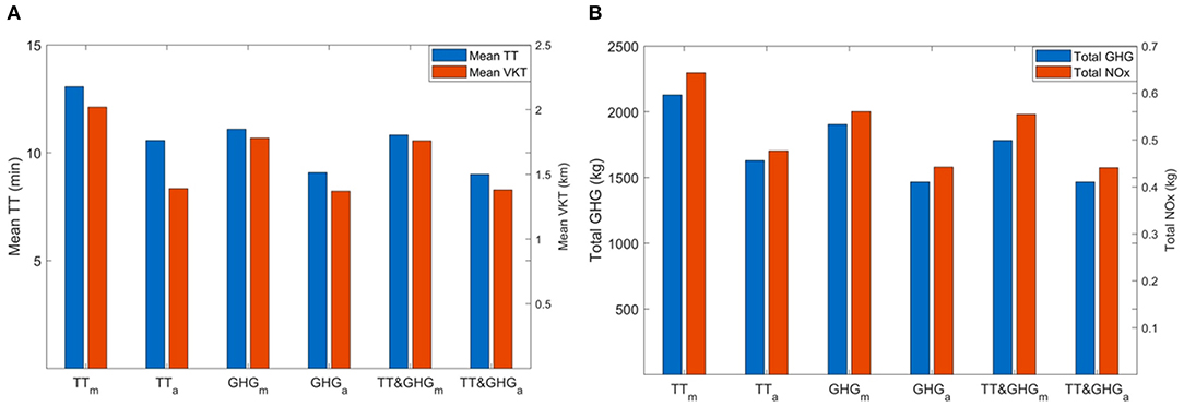
Figure 5. The impact of reactive and proactive routing strategies on the (A) mean TT and VKT and (B) total GHG and NOx.

The performance trend for reactive routing strategies was similar to that of the proactive routing strategies. From the worst to the best, TT was followed by GHG and TT&GHG in terms of the four performance indicators. Whether it was reactive or proactive routing, when TT was optimized the worst performance indicators were observed compared to when the routing objective was GHG or TT&GHG. The justification is that when TT was the objective all that matters was the spent TT on the links regardless of the VKT, GHG, and NOx indicators. Vehicles were distributed in the network to achieve the least TT, but this came at the cost of longer traveled distances and more produced GHG and NOx. Nevertheless, GHG_m and GHG_a introduced a decrease in the total produced GHG of 11 and 6% compared to TT_m and TT_a, respectively. This improvement can be directly linked to the marginal costing approach as in Equation (5), which takes into account not only the GHG ER but also speed on links. In other words, when the routing objective was GHG, the chosen links were defined based on the best combination of the GHG ER and speed that minimized the cost following Equation (7). The relationship between GHG and speed is quasi-convex (Djavadian et al., 2020) in which too low or too high speed would contribute to a higher GHG ER and higher GHG cost eventually. The multi-objective TT&GHG_m outperformed both TT_m and GHG_m in terms of the whole performance indicators. A reduction was observed in average TT, average VKT, total GHG, and total NOx of 17, 13, 16, and 14%, respectively, for the TT& GHG_m strategy compared to TT_m strategy. The reduction in the performance indicators of TT&GHG_m was marginal compared to the GHG_m routing strategy. TT&GHG routing objective controlled the TT cost and did not allow it to neglect the GHG objective. TT was thus reduced as long as it still satisfied the objective of reducing GHG. Paths of longer distances were not chosen as this triggered the increase in both the produced GHG and NOx like in TT routing strategy. TT&GHG_a was associated with reductions in the average TT, average VKT, total GHG, and total NOx of 15, 1, 10, and 7%, respectively, compared to TT_a. Comparing the best proactive routing strategy TT&GHG_a to the TT_m illustrates a reduction in average TT, average VKT, total GHG, and total NOx of 17, 22, 18, and 20%, respectively. With reference to the NOx variable, it has been found that the relationship between NOx and speed is also quasi-convex (Djavadian et al., 2020). Moreover, previous studies have confirmed that at high speeds NOx is sensitive to aggressive driving (Tu et al., 2019). Figure 5B shows that when GHG was part of the routing objective (GHG or TT&GHG), the produced NOx was less compared to when TT was the routing objective regardless of the routing protocol, reactive or proactive. It can be concluded that the experienced additional time and longer trips by vehicles in the case of reactive and proactive routing contributed to the increase in the produced GHG and NOx emissions.

5.3. Path Analysis

For this analysis, one vehicle was chosen randomly, and its reactive and proactive paths with different routing objectives were investigated. Comparing the reactive in Figure 6 with the proactive routes in Figure 7 for each of the objectives shows that there was more re-routing in the former contributing to longer trips and probably more time in the network as illustrated in section 5.2. The main explanation is that the cost of links was based on the current traffic conditions and did not consider the evolution of traffic in future.

FIGURE 6

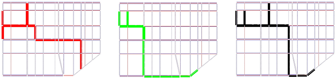
Figure 6. Reactive routes of a random vehicle subjected to different routing strategies: (A) TT, (B) GHG, and (C) TT&GHG.

FIGURE 7

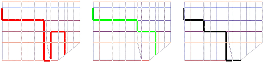
Figure 7. Proactive routes of a random vehicle subjected to different routing strategies: (A) TT, (B) GHG, and (C) TT&GHG.

In Figure 6, re-routing happened on the north-south links more frequently due to their higher capacity, which triggered higher speed (less TT), compared to the east-west links. This analysis supports the findings in Figure 5A, which demonstrates the decrease in average TT and VKT while proactive routing was adopted. Whether the routing protocol was reactive or proactive, comparing the length of the path of the TT to GHG and TT&GHG routing strategies illustrates that the length of the path of TT strategy was the longest. The main justification is that when TT was the objective, vehicles were distributed in the network utilizing uncongested links to achieve the least TT regardless of the traveled distance, produced GHG, and produced NOx. Figure 7A illustrates that instead of taking route a (east-west), of two links, route b (north-south), of five links, was chosen. The vehicle traversed an additional distance of around 700 m when taking route b compared to GHG_a and TT&GHG_a routing strategies. The speed of route b was around 38 km/h, while the speed of route a was around 1 km/h. This asserts that vehicles were distributed in the network to links of high speed to minimize the TT regardless of the traveled distance. When TT was the objective, the time spent on the links was optimized, while when GHG was part of routing objective the links of optimal speed were prioritized as long as the GHG marginal cost was minimized. The length of routes of the GHG_a and TT&GHG_a routing strategies was comparable as illustrated in Figures 7B,C, respectively.

5.4. Network Level Analysis

To examine the effect at the network level of the reactive and proactive routing strategies while adopting different routing objectives, average speed, produced GHG, and produced NOx over time were examined. In other words, at every minute, average speed, total GHG, and total NOx of the whole links in the network were estimated for this analysis. The demand was loaded at 7:45 a.m., and the total demand was in the network at around 8:00 a.m., which represented the peak of the congestion. Comparing Figure 8 to Figure 9, shows that the network has been loaded and unloaded quicker in the case of proactive routing.

FIGURE 8

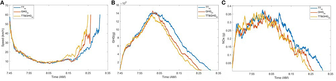
Figure 8. The Network under the different reactive routing strategies and its (A) speed, (B) GHG, and (C) NOx over time.

FIGURE 9

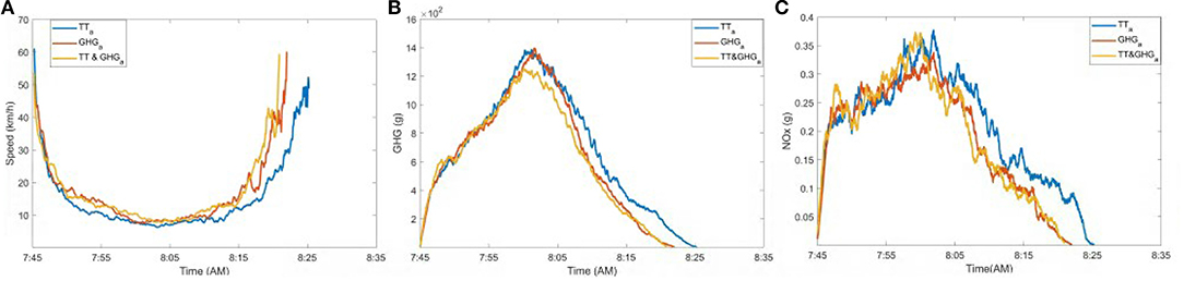
Figure 9. The Network under the different proactive routing strategies and its (A) speed, (B) GHG, and (C) NOx over time.

Particularly, for TT_m, the vehicles spent 15% more time in the network compared to TT_a. This finding is aligned with the analysis of the TT, VKT, GHG, and NOx in Figure 5 for TT_m compared to TT_a. Figure 6 demonstrates the additional re-routing in the case of reactive routing compared to the proactive routing strategies in Figure 7. The noticed additional re-routing in the case of TT_m, which triggered longer trip lengths compared to TT_a, contributed to the additional spent time in the network as well. The throughput over time of TT_m was less compared to GHG_m and TT&GHG_m. It took around 8 and 10.6% less time to load and unload the network for GHG_m and TT&GHG_m, respectively, compared to TT_m. The main explanation is that when travel time minimization was the objective, all link options were analyzed, and the final cost of travel time did not take into account the VKT as long as the objective was minimized. However, when GHG was the part of the optimization process, the links of optimal speed were prioritized and the re-routing averted. The GHG marginal cost as in Equation (5) made sure that vehicles spent the least amount of time and traveled the least distance while the objective was minimized, which is observed in Figures 6, 7 of the related strategies. The average speed till 8:10 a.m. of the reactive routing strategies in Figure 8A was almost identical for the three routing strategies, while GHG_a and TT&GHG_a were associated with a slightly higher speed than TT_a as in Figure 9. This asserts the importance and positive impact of the proactive routing, which takes into account the future state of traffic conditions in the network. After 8:10 a.m. and till the end of the simulation, the increase in speed for GHG_a and TT&GHG_a compared to TT_a was higher than in the case of the GHG_m and TT&GHG_m compared to TT_m. The reason is that the vehicles reached their destination faster in the case of proactive routing compared to reactive routing, which means less vehicles were in the network in the former case.

The main difference between Figure 8B and Figure 9B is that the period of time vehicles produced GHG was longer in the former, as the proactive routing included the future state of the traffic conditions and dealt with the changes proactively compared to the reactive routing. In addition, the GHG costing approach took into account not only the GHG ER but also the speed and VKT implicitly. The experienced additional time and VKT by vehicles in the case of TT_m, as shown in Figure 5A, contributed to the higher levels of GHG compared to GHG_m and TT&GHG_m in Figure 8B, especially after the congestion peak at 8:10 a.m. The number of vehicles in the network is an essential factor to keep in mind. On the other hand, comparing the GHG over time of TT_a to GHG_a and TT&GHG_a, illustrated less variation.

NOx over time followed the same trend of GHG over time and was associated with fewer emissions over time while the proactive routing was utilized as in Figure 9C compared to Figure 8C of the reactive routing strategies. For the NOx over time analysis, as shown in Figures 8C, 9C, the high values until around 8:00 a.m. were due to the high speed of the uncongested network. After 8:00 a.m., the number of vehicles and speed level controlled the produced NOx. At 8:00 a.m., the complete demand was in the network and the speed was the variable with direct impact on the produced NOx. It was observed that for TT_m in Figure 8C and TT_a in Figure 9C, NOx was higher than the cases when GHG or TT&GHG was the routing objective. This is because vehicles were directed to longer paths, but of higher speed to minimize the travel time. NOx is sensitive to aggressive driving (Tu et al., 2019), which makes higher speed links unfavorable. However, the reduction in the experienced TT and VKT in the network in the case of proactive routing means higher throughput over time. The higher throughput contributed to less NOx over time.

It can be concluded that using predicted link cost was associated with significant improvements at the network level. Furthermore, utilizing the GHG marginal cost, which takes into account not only the GHG ER but also the speed and VKT, was very effective and outperformed the travel time cost in terms of the whole performance indicators.

6. Conclusion and Potential Directions

Existing eco-routing studies are predominantly associated with limitations related to the aggregation level of the traffic flow and emission models, scale of the case study, used routing system (centralized), and the number of simultaneously optimized objectives (Alfaseeh and Farooq, 2020). Alfaseeh et al. (2019) and Djavadian et al. (2020) overcame these limitations and applied reactive multi-objective eco-routing strategies in a distributed routing framework with favorable outcomes. However, the technological advancements related to ICT and CAVs have not yet been exploited completely. This study thus suggested proactive multi-objective eco-routing strategies using a distributed routing system for CAVs (E2ECAV) (Farooq and Djavadian, 2019) to reduce the produced emissions. Predictive models of GHG ER and speed were developed and used. A deep-learning-based time series model, LSTM, was trained while systematically tuned. For sequential data, LSTM is known to be the most powerful recurrent NN architectures (Lipton et al., 2015). Furthermore, the LSTM model employed here outperformed the commonly used models, such as ARIMA (Alfaseeh et al., 2020).

The major findings of this study are as follows. Proactive routing strategies outperformed the reactive ones due to the inclusion of future traffic and environmental conditions in the route calculations. The paths of reactive routing strategies demonstrated a high degree of re-routing, as the cost did not consider the evolution of traffic and environmental states. Routing based on GHG as the objective was associated with noticeable reductions in average TT, average VKT, total GHG, and total NOx compared to the case where TT was the objective. This stems from the use of the marginal cost in Equation (5), which resulted in the best combination of speed, distance, and GHG ER on links that minimized the GHG cost. Re-routing was minimized when GHG was part of the optimization process as the increase in the VKT had a negative impact on the produced GHG. The GHG routing objective contributed to less TT and VKT, which led to less GHG and NOx in the network. For reactive and proactive routing, TT&GHG routing strategy introduced enhancements in terms of the four performance indicators compared to the TT routing strategy. Comparison of the former to the latter would be like comparing the system optimal (SO) to the user equilibrium (UE) (Papacostas and Prevedouros, 1993). Comparing the best proactive routing strategy, which optimized not only TT but also GHG, illustrated a reduction in average TT, average VKT, total GHG, and total NOx of 17, 21, 18, and 20%, respectively, when compared with the reactive routing aiming to minimize TT.

For future work, utilizing real data points from sensors instead of simulated data would result in higher heterogeneity in the data and ensure robustness in the models. The constrained eco-routing concept is an important aspect to be tackled and would illustrate the tradeoffs compared to the regular eco-routing application. As 100% CAVs MPR was employed in this study, the impact of different MPRs should be taken into account. The most preferable MPR of CAVs could vary from a traffic condition to another and this must be defined. The utilized predictive models in this study can be further enhanced by using more data points to represent the conditions of low frequency of occurrence. In addition, predictive models can be developed based on categorized characteristics, such as speed limit, number of lanes, etc., of links for further enhancements. With regards to the scalability aspect, it is suggested that proactive routing is applied in a larger network with both uninterrupted and interrupted traffic flow. Nevertheless, the predictive models should accommodate the difference between the two types of traffic flow. The employed distributed routing framework adopts only the V2I and I2I communication. The impact of incorporating the V2V communication is another suggestion for future work. Incorporating proactive routing strategies as an additional option in the personal navigation platforms would contribute to more efficient and sustainable transportation systems. Despite the strong contradiction between NOx and speed, including NOx as a routing objective is encouraged.

Data Availability Statement

The raw data supporting the conclusions of this article can be made available by the authors upon request.

Author Contributions

LA and BF: study conception and design, development of methodology, analysis and interpretation of results, and draft manuscript preparation. LA: running of the experiments and simulations and preparation of the data. BF: overall supervision. All authors reviewed the results and approved the final version of the manuscript.

Funding

This research was funded by the Ontario Early Researcher Award awarded to BF.

Conflict of Interest

The authors declare that the research was conducted in the absence of any commercial or financial relationships that could be construed as a potential conflict of interest.

Acknowledgments

Nikki Hera-Farooq helped us elevate the quality of our manuscript, for which we are grateful to her. We would also like to thank Dr. Shadi Djavadian for providing the source code for traffic microsimulation and E2ECAV used in this research.

Supplementary Material

The Supplementary Material for this article can be found online at: https://www.frontiersin.org/articles/10.3389/ffutr.2020.594608/full#supplementary-material

References

Aggarwal, C. C. (2018). Neural Networks and Deep Learning. New York, NY: Springer. doi: 10.1007/978-3-319-94463-0

CrossRef Full Text | Google Scholar

Alfaseeh, L., Djavadian, S., and Farooq, B. (2018). “Impact of distributed routing of intelligent vehicles on urban traffic,” in 2018 IEEE International Smart Cities Conference (ISC2) (Kansas, MO), 1–7. doi: 10.1109/ISC2.2018.8656941

CrossRef Full Text | Google Scholar

Alfaseeh, L., Djavadian, S., Tu, R., Farooq, B., and Hatzopoulou, M. (2019). “Multi-objective eco-routing in a distributed routing framework,” in 2019 IEEE International Smart Cities Conference (ISC2) (Casablanca), 747–752. doi: 10.1109/ISC246665.2019.9071744

CrossRef Full Text | Google Scholar

Alfaseeh, L., and Farooq, B. (2020). Multifactor taxonomy of ecorouting models and future outlook. J. Sensors 2020:4362493. doi: 10.1155/2020/4362493

CrossRef Full Text | Google Scholar

Alfaseeh, L., Tu, R., Farooq, B., and Hatzopoulou, M. (2020). Greenhouse gas emission prediction on road network using deep sequence learning. arXiv:2004.08286v1. doi: 10.1016/j.trd.2020.102593

CrossRef Full Text | Google Scholar

Amarpuri, L., Yadav, N., Kumar, G., and Agrawal, S. (2019). “Prediction of co2 emissions using deep learning hybrid approach: a case study in Indian context,” in 2019 Twelfth International Conference on Contemporary Computing (IC3) (Raleigh, NC), 1–6. doi: 10.1109/IC3.2019.8844902

CrossRef Full Text | Google Scholar

Ameyaw, B., Yao, L., Oppong, A., and Agyeman, J. K. (2019). Investigating, forecasting and proposing emission mitigation pathways for co2 emissions from fossil fuel combustion only: a case study of selected countries. Energy Policy 130, 7–21. doi: 10.1016/j.enpol.2019.03.056

CrossRef Full Text | Google Scholar

Barlow, G. J., and Kennett, C. (2019). Optimizing for everyone using cooperative adaptive control.

Google Scholar

Ben-Akiva, M., Bierlaire, M., Burton, D., Koutsopoulos, H. N., and Mishalani, R. (2001). Network state estimation and prediction for real-time traffic management. Netw. Spat. Econ. 1, 293–318. doi: 10.1023/A:1012883811652

CrossRef Full Text | Google Scholar

Bilali, A., Isaac, G., Amini, S., and Motamedidehkordi, N. (2019). Analyzing the impact of anticipatory vehicle routing on the network performance. Transport. Res. Proc. 41, 494–506. doi: 10.1016/j.trpro.2019.09.082

CrossRef Full Text | Google Scholar

Bottom, J. A. (2000). Consistent anticipatory route guidance (Ph.D. thesis). Massachusetts Institute of Technology, Cambridge, MA, United States.

Google Scholar

Campbell, P., Zhang, Y., Yan, F., Lu, Z., and Streets, D. (2018). Impacts of transportation sector emissions on future us air quality in a changing climate. Part I: Projected emissions, simulation design, and model evaluation. Environ. Pollut. 238, 903–917. doi: 10.1016/j.envpol.2018.04.020

CrossRef Full Text | Google Scholar

Claes, R. (2015). Anticipatory vehicle routing (Ph.D. thesis). KU Leuven, Science, Engineering & Technology.

Google Scholar

Council of Ministers Transportation and Highway Safety (2012). The High Cost of Congestion in CANADIAN CITIES. Council of Ministers Transportation and Highway Safety.

Google Scholar

Cox, L. (1999). Nitrogen Oxides (NOx) Why and How They Are Controlled. Raleigh, NC: Diane Publishing.

Google Scholar

Djavadian, S., and Farooq, B. (2018). “Distributed dynamic routing using network of intelligent intersections,” in ITS Canada ACGM (2018) (Niagara Fall, NY).

Google Scholar

Djavadian, S., Tu, R., Farooq, B., and Hatzopoulou, M. (2020). Multi-objective eco-routing for dynamic control of connected & automated vehicles. Transport. Res. Part D 87, 1–21. doi: 10.1016/j.trd.2020.102513

CrossRef Full Text | Google Scholar

DMG (2011). Transportation Tomorrow Survey.

Google Scholar

Duan, Y., Lv, Y., and Wang, F.-Y. (2016). “Travel time prediction with lstm neural network,” in 2016 IEEE 19th International Conference on Intelligent Transportation Systems (ITSC) (Rio de Janeiro), 1053–1058. doi: 10.1109/ITSC.2016.7795686

CrossRef Full Text | Google Scholar

Elbery, A., Rakha, H., ElNainay, M. Y., Drira, W., and Filali, F. (2016). “Eco-routing: an ant colony based approach,” in VEHITS (2016) (Rome), 31–38. doi: 10.5220/0005778900310038

CrossRef Full Text | Google Scholar

EPA, U. (2020a). Overview of Greenhouse Gases. Greenhouse gas emissions.

EPA, U. (2020b). Sources of Greenhouse Gas Emissions.

Farooq, B., and Djavadian, S. (2019). Distributed Traffic Management System with Dynamic End-to-End Routing.

Google Scholar

Gu, Y., Lu, W., Qin, L., Li, M., and Shao, Z. (2019). Short-term prediction of lane-level traffic speeds: a fusion deep learning model. Transport. Res. Part C 106, 1–16. doi: 10.1016/j.trc.2019.07.003

CrossRef Full Text | Google Scholar

Guerrero-Ibá nez, J., Zeadally, S., and Contreras-Castillo, J. (2018). Sensor technologies for intelligent transportation systems. Sensors 18:1212. doi: 10.3390/s18041212

PubMed Abstract | CrossRef Full Text | Google Scholar

Hermans, M., and Schrauwen, B. (2013). “Training and analysing deep recurrent neural networks,” in Advances in Neural Information Processing Systems (Lake Tahoe), 190–198.

Google Scholar

Hutter, F., Lücke, J., and Schmidt-Thieme, L. (2015). Beyond manual tuning of hyperparameters. KI-Künstliche Intell. 29, 329–337. doi: 10.1007/s13218-015-0381-0

CrossRef Full Text | Google Scholar

International Joint Commission (2012). Canada/United States Air Quality Agreement: Progress Report 2012. International Joint Commission.

Google Scholar

Kaufman, D. E., Smith, R. L., and Wunderlich, K. E. (1991). “An iterative routing/assignment method for anticipatory real-time route guidance,” in Vehicle Navigation and Information Systems Conference, 1991, Vol. 2, 693–700. doi: 10.4271/912815

CrossRef Full Text | Google Scholar

Kim, K., Kwon, M., Park, J., and Eun, Y. (2016). Dynamic vehicular route guidance using traffic prediction information. Mobile Inform. Syst. 2016:3727865. doi: 10.1155/2016/3727865

CrossRef Full Text | Google Scholar

Kingma, D. P., and Ba, J. (2014). Adam: a method for stochastic optimization. arXiv preprint arXiv:1412.6980.

Google Scholar

Liang, Z., and Wakahara, Y. (2014). Real-time urban traffic amount prediction models for dynamic route guidance systems. EURASIP J. Wireless Commun. Netw. 2014:85. doi: 10.1186/1687-1499-2014-85

CrossRef Full Text | Google Scholar

Lipton, Z. C., Berkowitz, J., and Elkan, C. (2015). A critical review of recurrent neural networks for sequence learning. arXiv preprint arXiv:1506.00019.

Google Scholar

Liu, S., and Qu, Q. (2016). Dynamic collective routing using crowdsourcing data. Transport. Res. Part B 93, 450–469. doi: 10.1016/j.trb.2016.08.005

CrossRef Full Text | Google Scholar

Luo, L., Ge, Y.-E., Zhang, F., and Ban, X. J. (2016). Real-time route diversion control in a model predictive control framework with multiple objectives: traffic efficiency, emission reduction and fuel economy. Transport. Res. Part D 48, 332–356. doi: 10.1016/j.trd.2016.08.013

CrossRef Full Text | Google Scholar

Ma, X., Tao, Z., Wang, Y., Yu, H., and Wang, Y. (2015). Long short-term memory neural network for traffic speed prediction using remote microwave sensor data. Transport. Res. Part C 54, 187–197. doi: 10.1016/j.trc.2015.03.014

CrossRef Full Text | Google Scholar

Mahmassani, H. S. (1994). Development and testing of dynamic traffic assignment and simulation procedures for ATIS/ATMS applications.

Google Scholar

Mane, A. S., and Pulugurtha, S. S. (2018). “Link-level travel time prediction using artificial neural network models,” in 2018 21st International Conference on Intelligent Transportation Systems (ITSC) (Yokohama), 1487–1492. doi: 10.1109/ITSC.2018.8569731

CrossRef Full Text | Google Scholar

Pan, J., Popa, I. S., Zeitouni, K., and Borcea, C. (2013). Proactive vehicular traffic rerouting for lower travel time. IEEE Trans. Vehicul. Technol. 62, 3551–3568. doi: 10.1109/TVT.2013.2260422

CrossRef Full Text | Google Scholar

Pao, H.-T., and Tsai, C.-M. (2011). Modeling and forecasting the co2 emissions, energy consumption, and economic growth in Brazil. Energy 36, 2450–2458. doi: 10.1016/j.energy.2011.01.032

CrossRef Full Text | Google Scholar

Papacostas, C. S., and Prevedouros, P. D. (1993). Transportation engineering and planning.

Google Scholar

Pascanu, R., Gulcehre, C., Cho, K., and Bengio, Y. (2013). How to construct deep recurrent neural networks. arXiv preprint arXiv:1312.6026.

Google Scholar

Rahman, A., and Hasan, M. M. (2017). Modeling and forecasting of carbon dioxide emissions in Bangladesh using autoregressive integrated moving average (Arima) models. Open J. Stat. 7, 560–566. doi: 10.4236/ojs.2017.74038

CrossRef Full Text | Google Scholar

Rakha, H., Ahn, K., and Moran, K. (2012). Integration framework for modeling eco-routing strategies: logic and preliminary results. Int. J. Transport. Sci. Technol. 1, 259–274. doi: 10.1260/2046-0430.1.3.259

CrossRef Full Text | Google Scholar

Ran, X., Shan, Z., Fang, Y., and Lin, C. (2019). An lstm-based method with attention mechanism for travel time prediction. Sensors 19:861. doi: 10.3390/s19040861

PubMed Abstract | CrossRef Full Text | Google Scholar

Reimers, N., and Gurevych, I. (2017). Optimal hyperparameters for deep lstm-networks for sequence labeling tasks. arXiv preprint arXiv:1707.06799.

Google Scholar

Robert, C. (2014). Machine Learning, A Probabilistic Perspective. Taylor & Francis. doi: 10.1080/09332480.2014.914768

CrossRef Full Text | Google Scholar

Snoek, J., Larochelle, H., and Adams, R. P. (2012). “Practical bayesian optimization of machine learning algorithms,” in Advances in Neural Information Processing Systems, 2951–2959.

Google Scholar

Statistics Canada (2018). Average Usual Hours and Wages by Selected Characteristics, Monthly, Unadjusted for Seasonality. Statistics Canada.

The World Bank (2019). Carbon Pricing Dashboard. The World Bank.

Toronto Foundation (2020). Toronto's Vital Signs. Toronto Foundation.

Treiber, M., Hennecke, A., and Helbing, D. (2000). Congested traffic states in empirical observations and microscopic simulations. Phys. Rev. E 62, 1805–1824. doi: 10.1103/PhysRevE.62.1805

PubMed Abstract | CrossRef Full Text | Google Scholar

Tu, R., Alfaseeh, L., Djavadian, S., Farooq, B., and Hatzopoulou, M. (2019). Quantifying the impacts of dynamic control in connected and automated vehicles on greenhouse gas emissions and urban No2 concentrations. Transport. Res. Part D 73, 142–151. doi: 10.1016/j.trd.2019.06.008

CrossRef Full Text | Google Scholar

Tudor, C. (2016). Predicting the evolution of co2 emissions in Bahrain with automated forecasting methods. Sustainability 8:923. doi: 10.3390/su8090923

CrossRef Full Text | Google Scholar

United States Environmental Protection Agency (2020). How does MOVES Calculate CO2 and CO2 Equivalent Emissions? Available online at: https://www.epa.gov/moves/how-does-moves-calculate-co2-and-co2-equivalent-emissions (accessed July 9, 2020).

PubMed Abstract | Google Scholar

USEPA (2015). Exhaust Emission Rates for Light-Duty on-Road Vehicles in Moves2014: Final Report. United States Environmental Protection Agency.

Vlahogianni, E. I., Karlaftis, M. G., and Golias, J. C. (2014). Short-term traffic forecasting: where we are and where we're going. Transport. Res. Part C 43, 3–19. doi: 10.1016/j.trc.2014.01.005

CrossRef Full Text | Google Scholar

Wang, J., Elbery, A., and Rakha, H. A. (2019). A real-time vehicle-specific eco-routing model for on-board navigation applications capturing transient vehicle behavior. Transport. Res. Part C 104, 1–21. doi: 10.1016/j.trc.2019.04.017

CrossRef Full Text | Google Scholar

Wu, J., Chen, X.-Y., Zhang, H., Xiong, L.-D., Lei, H., and Deng, S.-H. (2019). Hyperparameter optimization for machine learning models based on Bayesian optimization. J. Electron. Sci. Technol. 17, 26–40.

Google Scholar

Yang, X., and Recker, W. W. (2006). Modeling dynamic vehicle navigation in a self-organizing, peer-to-peer, distributed traffic information system. J. Intell. Transport. Syst. 10, 185–204. doi: 10.1080/15472450600981041

CrossRef Full Text | Google Scholar

Yao, B., Chen, C., Cao, Q., Jin, L., Zhang, M., Zhu, H., et al. (2017). Short-term traffic speed prediction for an urban corridor. Comput. Aided Civil Infrastruct. Eng. 32, 154–169. doi: 10.1111/mice.12221

CrossRef Full Text | Google Scholar

Zegeye, S. K., De Schutter, B., Hellendoorn, H., and Breunesse, E. (2009). “Model-based traffic control for balanced reduction of fuel consumption, emissions, and travel time,” in Proceedings of the 12th IFAC Symposium on Transportation Systems (2009), 149–154. doi: 10.3182/20090902-3-US-2007.0018

CrossRef Full Text | Google Scholar

Zhang, G. P. (2003). Time series forecasting using a hybrid arima and neural network model. Neurocomputing 50, 159–175. doi: 10.1016/S0925-2312(01)00702-0

CrossRef Full Text | Google Scholar

Zhang, T., Jin, J., Yang, H., Guo, H., and Ma, X. (2019). “Link speed prediction for signalized urban traffic network using a hybrid deep learning approach,” in 2019 IEEE Intelligent Transportation Systems Conference (ITSC), 2195–2200. doi: 10.1109/ITSC.2019.8917509

CrossRef Full Text | Google Scholar

Zhang, X., and Rice, J. A. (2003). Short-term travel time prediction. Transport. Res. Part C 11, 187–210. doi: 10.1016/S0968-090X(03)00026-3

CrossRef Full Text | Google Scholar

Zhao, J., Zhang, J., Jia, S., Li, Q., and Zhu, Y. (2011). “A Mapreduce framework for on-road mobile fossil fuel combustion co2 emission estimation,” in 2011 19th International Conference on Geoinformatics, 1–4. doi: 10.1109/GeoInformatics.2011.5980759

CrossRef Full Text | Google Scholar