Moving Array Traffic Probes

1. Introduction

The fast-approaching advent of Autonomous Vehicles (AVs) will have many benefits as well as unforeseen disadvantages and risks (Davidson and Spinoulas, 2015; Levinson and Krizek, 2017; Liu et al., 2017; Morando et al., 2018). After several years of development, the well-known Google/Waymo Car project has gained significant momentum and has autonomously driven over 16 million autonomously driven km as of 2018 (Korosec, 2018). Within the next decade, it is expected that AVs will be on the market and on public roads.

Given that such a shift in transport will probably require important changes in transport networks (Fagnant and Kockelman, 2015), AVs' potential in supplying accurate and detailed traffic data may be invaluable in facilitating these changes. One of the neglected side-benefits of AVs is their potential to act as moving array “probes” collecting traffic data which can then be utilized to map real-time traffic conditions as well as long-term traffic information for planning and other traffic engineering purposes. Unlike traditional vehicle probes, moving array probes can collect data on their surroundings as well as their own state. While traditional vehicles can in theory be equipped as moving array probes, autonomous vehicles will be such by default, providing increasing streams of data.

At present, there are many methods of collecting traffic data, but most of them are time and labor consuming, expensive, and localized. This study explores the possibility of using AV data as a reliable, economical, and wide-coverage alternative to existing methods. This is chiefly undertaken from the perspective of a single AV and its corresponding capabilities, given the relatively small number of AVs which will impact on public roads initially. In addition, the benefits of greater numbers of AV probes are also explored. Following this investigation, we recommend future research into moving array traffic probes.

The remainder of this paper is structured as follows. First, 2 reviews some of the existing data collection methods and demonstrates the current research on traffic probes. Then, sections 3, 4 state the methodologies that will be used to simulate scenarios and to validate the model. In 5, results and discussion are proposed through the analysis of the percentage absolute errors among three different cases. Finally, 6 summarizes the findings and indicates the further objective of moving array traffic probes.

2. Review of Data Collection Methods

Leduc (2008) distinguishes between traditional in-situ data collection methods such as pneumatic road tubes and manual counts and floating car data which provides traffic data from moving probe vehicles. Seo et al. (2017) classified Traffic State Estimation (TSE) into stationary data methods which collects data at installed locations of stationary sensors and mobile data methods which collect data on specific vehicles along their trajectories. To differentiate the potential of AV probes, we propose a new data collection method categorization system with three classes:

• static array (Eulerian frame),

• moving point (Lagrangian frame) and

• moving array.

2.1. Static Array (Eulerian Frame)

Static array consists of those traditional data collection methods which collect an array of data relating to multiple surrounding vehicles from a static location, such as pneumatic tubes and manual counts. Antoniou et al. (2011) classified current technologies into three categories:

• point sensors,

• point-to-point sensors, and

• area-wide sensors.

Point sensors include instruments such as inductive loop detectors, radar, infrared, ultrasound, video image detection, and weigh in motion systems. These instruments work individually and gather data without the aid of a secondary system. There are a number of newer point-sensor technologies, primarily light detection and ranging (LIDAR), which are also used in AVs across the board (Schaub, 2018).

Point-to-point sensors involve data collectors such as automated vehicle identification (AVI) and license plate recognition, where a sensor (such as the electronic tag in the case of AVI, and the camera in license plate recognition) transmits a vehicle's location to a secondary system which can then analyse and use that data.

Area-wide sensors tend to be more experimental and are usually large-scale networks of point-to-point sensors, which contain the location data of a moving sensor (such as the mobile phone or GPS in a vehicle) being accessed by a secondary system in stations (i.e., cell towers) for many vehicles.

For most static detectors, traffic counts, vehicle occupancy, and instantaneous speeds of vehicles at the location can be measured. This disaggregated information needs to be converted into an average traffic state at a particular sample time (Seo et al., 2017).

Macroscopically, Makigami et al. (1971) described traffic flow variables based on a three-dimensional representation so that those macroscopic variables can be derived by recorded location, time, and cumulative vehicle counts. The detectors are widely used to collect data because of their convenience and feasibility in practice, however, the current spacing ranges from some hundred meters to several kilometers due to high deployment and maintenance fees of the sensors, such space resolution may cause the collected data to be insufficient (Wang and Papageorgiou, 2005). Moreover, the frequent missing or incorrect counts from static detectors is another data accuracy and quality problem (Chen et al., 2003).

2.2. Moving Point (Lagrangian Frame)

Moving point observations are most commonly seen as floating car data, where point data is continuously collected by a moving probe. However, that data only relates to the probe itself, not the surrounding traffic. Despite limitations, floating car data can collect a range of traffic-related information along their trajectories providing individual position and velocity information, for instance by employing smartphones and GPS devices on-board probes. With calibrated fundamental diagrams or similar relations (Nanthawichit et al., 2003; Work et al., 2010), traffic state variables like density and flow can be estimated. There have also emerged many fundamental diagram-free TSEs based on streaming-data-driven methods to estimate macroscopic variables (Coifman, 2003; Seo et al., 2015b; Bekiaris-Liberis et al., 2016). Deployment of deep learning and V2X communications may improve traffic state estimation (Sanguesa et al., 2015; Lou et al., 2016; Lin et al., 2018; Xu et al., 2020), but there is no evidence that such technologies will be ubiquitous nor feasible in the near term. Simply speaking, a probe vehicle's route can be reconstructed based on a series of locations transmitted by the probe to a secondary system for estimation. This was tested, among other cases, in a Beijing study, where it was found that location data from taxi probe vehicles could be used to establish reasonably accurate probe routes to the point of making cross-referenced geographical data potentially irrelevant (He and Zheng, 2017). Another use of floating car data that has been investigated is its ability to estimate route travel time. From an array of location data for a given probe, a route and travel time can theoretically be estimated (Rahmani et al., 2015). In the meanwhile, methods for estimating the demand for traffic networks using floating car data have also been investigated with some success (Carrese et al., 2017).

One of the main limitations other than the small number of probe vehicles is the low sampling frequency due to technological restrictions. This leads to significant uncertainties about the actual path taken by the vehicle and the speed of the vehicle (as only average speed can be calculated) (Jenelius and Koutsopoulos, 2015). Also, no information regarding traffic density is available from most floating car studies without calibrated fundamental diagrams. However, even when mapping from velocity to density through fundamental diagrams, especially in free flow scenarios, the estimation will have errors (Herrera and Bayen, 2010).

2.3. Moving Array: Moving Array Probes

A third class is the moving array—in that the data collection device moves and collects data relating to multiple surrounding vehicles (an array of data), not just the probe itself. While in principle, manual-driven instrumented vehicles could also serve as moving array probes, in practice, we expect the moving array data to come free with AVs (Qiu et al., 2010; Cao et al., 2011). At present instrumented vehicles can assess driver behavior (such as car-following and reaction time) by video cameras and LIDAR when following preceding cars (Ma and Andréasson, 2006; Soria et al., 2014; Schorr et al., 2017). Few of them can measure speeds and trajectories within their detection areas by using LIDAR and GPS (Xuan and Coifman, 2012; Coifman et al., 2016). But in practice, we expect the moving array data to come free with AVs without extra labor and equipment installation costs.

The limitations of floating cars could be mitigated by moving array AV probes, which produce information regarding traffic flow and density inherently and do not necessarily need to accumulate data or use fundamental diagrams to estimate this information.

A fundamental difference between Lagrangian and Eulerian data collection frames and moving array AV probes is that the previous systems only collect data concerning the probe vehicle itself, or (as for static traffic counters) collect data on multiple vehicles in one location. The array of sensors necessarily built into an AV have not yet been widely recognized as a potential source of traffic data.

Currently, there has been a modest amount of research into the use of moving array probes. Moving array probes can estimate traffic flow characteristics by detecting the headway to the leading vehicle (Seo et al., 2015b) or by combining stationary and moving probes collected data together based on the Point-Observations N (PON) estimation (van Erp et al., 2018) both without assumed fundamental diagrams or other flow models.

Moreover, LIDAR data can be interpreted to give useful information about the status of the surrounding traffic (Cetin et al., 2017), including detection and classification of vehicles (as distinct from the ground and other surrounding objects) and establishing trajectories for the detected vehicles with various algorithms. However, this methodology depends upon a reasonable number' of probes to be collecting data in a given area in order to estimate traffic density. Our study makes no such assumption and considers the case where only one AV is operating—to explore the data collection possibilities of a single probe. This is particularly useful for the early stages of the integration of AVs on public roads, when they will be relatively scarce.

Another recent report also investigates the collection of data from AVs (Chen et al., 2017) which focuses more on traffic data collected for the immediate use of the AV itself and is highly theoretical. The present investigation aims to exploit AV collected data for more general purposes and aggregate over a longer period of time to generate both real-time and long-term information for the purposes of planning and traffic management.

3. Method

Traditional traffic data collection consists of vehicle flows, mean densities, velocities, and classifications (generally light vehicles vs. heavy vehicles). Edie (1963) focused on the first three parameters for a region D within given ranges of space and time.

The field to be explored is the use of data from already inbuilt sensors in AVs as a potential, soon-to-be widespread, traffic information source. The three fundamental parameters to be considered are flow q, density k, and velocity u. As such, they formed the primary objects of data collection for the AV probe model as follows:

$\begin{array}{ll}\begin{array}{c}{q}_D=\frac{{\displaystyle {\sum }_i{d}_i}}{A_D};k_D=\frac{{\displaystyle {\sum }_i{r}_i}}{A_D};u_D=\frac{q_D}{k_D}\end{array}& (1)\end{array}$

where:

D is selected study region in the time-space plot;

q_D is the space-mean flow in region D in veh/h;

k_D is the space-mean density in region D in veh/km;

u_D is the space-mean speed in region D in km/h;

d_i is the travel distance of vehicle i in region D in veh·km;

r_i is the time spent of vehicle i in region D in veh·h;

A_D is the time-space area of region D in km·h.

In AV probes, at present LIDAR is assumed to be the primary data collection method, with a visible radius of 100 m over all 360°. This system works by rapidly rotating an array of lasers which reflects off surrounding objects. It builds up information about the surrounding environment as a series of dynamic points. For example, it measures the distance to target vehicles by calculating how far the laser travels to and reflects back. For speed measurements, LIDAR sends out two laser pulses successively and compares the change in distance after receiving the pulses. The speed is then calculated by the change in distance divided by the time between two pulses. LIDAR counts the number of vehicles by capturing the point cloud and extracting moving vehicles within its detection range.

Conceptually, how an AV probe detects surrounding vehicles may be seen in Figure 1. Following Cetin et al. (2017), partially visible vehicles are still able to be accounted for in the vehicle recognition system.

FIGURE 1

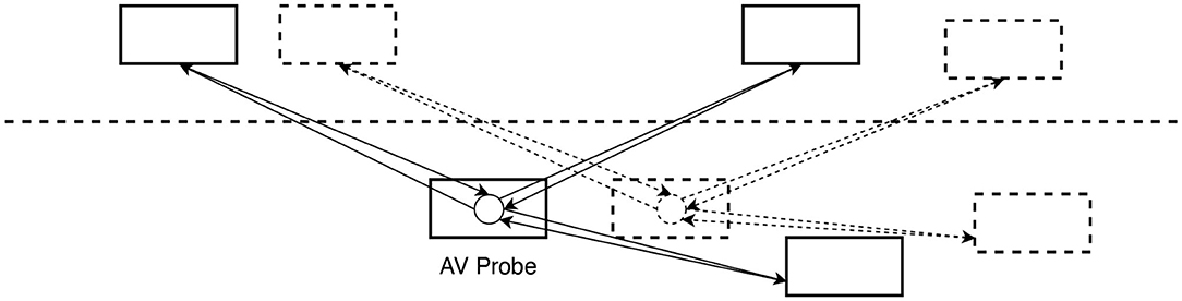
Figure 1. How LIDAR detects vehicles (arrows represent lasers being sent and reflected).

In this study, vehicle trajectories are computed based on the tracking of successive locations for given vehicles according to Cetin et al. (2017). Assuming this method, the vehicles within the visible radius will be classified into eastbound and westbound vehicles. These are treated separately as traffic conditions vary based on the direction of travel.

For traffic traveling in the same direction as the probe, the density is calculated based on the number of vehicles along a distance during a specific period. The speed of the vehicles (in the direction of travel) at the sample location is assumed to be an average of the probe vehicle speed itself and that of the surrounding vehicles (calculated based on their trajectories). Flow is the product of density and speed for both local and global scenarios in study region D. We assume that the global parameter measurement reflects the “ground-truth” situation while the local measurement is biased. The AV detection errors between two measurements can then be investigated in different scenarios.

$\begin{array}{ll}{u}_D=\frac{u_{pr}+{\displaystyle \sum u_{nm}}}{N_D};k_D=\frac{N_D}{l_D};q_D=u_D\times k_D& (2)\end{array}$

where:

u_pr is the speed of the single probe itself;

u_nm is the speed of other vehicles in study region D;

N_D is the number of vehicle counts in region D;

l_D is the interval length of space in region D.

To explain the estimation errors under such heterogeneous traffic conditions, we introduce the equilibrium curve of the fundamental diagram for analysis. When there is a transition between two different states in the diagram, a shockwave occurs with the wave speed w:

$\begin{array}{ll}w=\frac{\Delta q}{\Delta k}& (3)\end{array}$

in which:

w is the wave speed between two different states;

Δq is the change in flow between two states;

Δk is the change in density (concentration) between two states.

In a q-k plot, the wave speed w represents the slope of the shockwave between two states (Leutzbach, 1988). In free-flow conditions, due to the heterogeneous conditions, vehicles often platoon rather than distribute uniformly. Therefore, mean global densities over space could be impacted so that a shockwave occurs between two different states of free-flow conditions (shown in Figure 2).

FIGURE 2

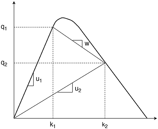
Figure 2. The wave speed in a fundamental diagram.

At the boundary of the free-flow state and the jam state, the critical density k_c (density at the capacity state) determines whether there appears a state transition. Once the mean density exceeds a critical point ($\bar{k}>k_c$), an upstream stop-and-go wave will then form backwards, and its queue accumulates when the fraction of mean density and critical density increases until jam conditions.

For a single probe existing in the road, it is initially hypothesized that there would firstly be an increase of absolute error in a probe's measurements of density, speed, and flow in the free-flow state. The reason behind this hypothesis is that a high error is expected with the low coverage scenario because traffic flow heterogeneity would dominate in these scenarios. That is, in free-flow situations, there are few sections with localized clusters but large sections with few or even no vehicles at all. A probe cannot accurately detect the information from the less representative observations because it is more likely to be a part of the locally high density flow. For these situations, the probe tends to over-estimate the overall density, in the meanwhile, the speed is under-estimated by the blocked probe together with other slow–moving vehicles.

The opposite extreme situation of such observation bias is a jam density situation, where the road coverage is at 100%. In such cases, it was expected that probe measurement error would approach 0 since the traffic conditions are perfectly homogeneous and the probe's visible sample is perfectly representative of the prevailing conditions.

However, the occurrence of inhomogeneous stop-and-go waves mainly caused by driver lane-changing behaviors in relative high road coverage rates also impacts on the accuracy of probe data collection. When the road coverage exceeds a specific state where the maximum flow rate exists, stop-and-go waves appear to slow down or stop the vehicles (sometimes including the probe) so that the density is over-estimated and the speed is under-estimated by the probe.

This phenomenon led to the consequence that probe error would not simply decrease from a high point under low road coverage conditions, to zero as traffic approached jam density conditions. It should follow another tendency with the increase of road coverage.

Compared with the single probe, the inductive loop detector had substantially lower error for low road coverage conditions, because it is not subject to the same degree of observation bias, in other words, it is less likely to be within an area of low density. Similarly, the loop has the more accurate density measurements in road coverage associated with shockwaves, because it does not suffer from the probe's increased likelihood of being stuck within an area of congestion rather than an area of free flow. Thus, the static nature of the loop detector may, purely from the perspective of accuracy, be seen as an advantage over the moving probe. However, loop detectors are expensive to install and only monitor a small area of the road, which are difficult for wide utilization, while data from AVs could be theoretically free, abundant, and sourced across a vast area. We expect future research can develop calibration methods to correct for observation bias produced from raw measurements.

To extend the theory from the one-directional model to the two-directional model, it was important to establish the consistency between two models. Therefore, 50,000-timestep tests were run for a range of road cover percentages, in order to plot an absolute error curve for a single probe measuring the density, speed, and flow of concurrent traffic only. This curve could then be compared with that plotted for the one-directional model. Although there is an evident fluctuation for the two-directional curve around the 20% coverage mark and there is some difference in the magnitudes of the error between the two curves, these issues are the result of different sample sizes for the two curves and do not affect the conclusion that the same traffic characteristics apply in both models.

4. Simulation Study

Three primary simulation scenarios were undertaken:

• Scenario 1: One probe operating in a one-directional pipeline;

• Scenario 2: Multiple probes operating in a one-directional pipeline; and

• Scenario 3: One probe operating in a two-directional pipeline.

As pipelines, these involve a length of road with no intersections. Moreover, the simulations are effectively circular pipelines, in which vehicles that reach the end of the pipeline reappear back at the beginning and continue driving. Future studies should explore further complex scenarios. The base model adapts Wilensky et al. (1998)'s “Traffic Two Lanes” model of two lanes of traffic moving in one direction, with an adjustable number of vehicles and acceleration/deceleration rates. The positions of all agents are randomly-distributed instead of homogeneously-distributed, consistent with reality. Each agent in Wilensky et al. (1998)'s model moves forward based on its speed and preset acceleration/deceleration until it reaches the speed of its leading vehicle. The model also allows for vehicles to change lanes when they are obstructed by slower moving vehicles ahead. The other adjustable element of the model is the vehicle “patience.” This model defines the “patience” variable as the number of times when any vehicle's speed is being restricted by vehicles ahead. If the traffic flow is congested, drivers will quickly lose their patience and frequently change lanes. Each vehicle has a slightly different speed that it is attempting to reach, which reflects a distribution of driver personalities. The model is implemented in NetLogo.

The model distance is given in units of cells, equivalent to a standard vehicle length (4.5 m), and time in units of timesteps. Furthermore, the timestep has been related to real-time units such that the average speed of vehicles in the model is assumed as 60 km/h. Given that the preset average speed of vehicles within the model is 0.6 cells per timestep, a timestep is taken to be 0.162 s or 0.000045 h. The unit length of road that is used to calculate density within the model is 44 cells (the length visible to a single probe). More parameter setting details are shown in Table 1.

TABLE 1

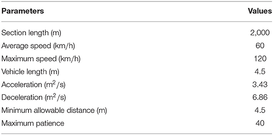
Table 1. Simulation parameter settings.

In order to design three different simulation scenarios, substantial additions and modifications were required to the traffic model. For Scenario 1 (single probe in one-directional pipeline), the road is widened to three lanes and the vehicle defined in the base model as the “selected-car” is taken to be the probe vehicle driving along the road with other traffic, but with no other probe vehicles. The model is updated such that the three primary traffic parameters: density, speed, and flow are measured at every timestep by both the probe vehicle and the system's spatially-fixed observers.

Density is measured by the probe by counting the number of vehicles (including itself) within a radius of 22 cells (model unit of distance) or approximately 100 m, while “ground-truth” is measured by the overall observer as the number of vehicles on the pipeline (of length 440 cells or nearly 2 km) divided by 10.

The freeway stretch length is taken to be 2 km, which has been used as the boundary of short and long stretches by previous TSE investigations (Cremer, 1991). We first test how well the moving array performs on a road of this length. Future research can explore alternative stretch lengths.

It was assumed that the observer measure is the “true” density, then the probe measure, which is subjective (i.e., from the perspective of the vehicle, and time-weighted, and so depends on how much time is spent in various conditions) is compared with it, and an “error” is calculated. Throughout, the Mean Absolute Percentage Error (MAPE) between the probe and the overall observer is estimated. Note that these density measurements are made by both the probe and the observer at each timestep (model time unit), and most simulations were run for a duration of 5,000 timesteps. Speed is measured by the probe by detecting the speed of all vehicles around it within a 22-cell radius and calculating a mean of these. The observer speed is simply the space-mean speeds of all vehicles on the pipeline. At each timestep, the probe multiplies density and speed to calculate a flow for the vehicles within its visible radius for each given timestep. A similar function is performed by the overall observer, and the averaged flows over the whole simulation can again be compared and the error calculated.

For Scenario 2 (multiple probes in a one-directional pipeline), a three-lane configuration is also used. The methods of collecting parameter measurements for both the probe(s) and the overall observer were the same as for Scenario 1. For each experiment, the output is collected from 1, 2, 10, 20, and 100 probes (all vehicles are probes). Then the measurements made by multiple probes can be compared with the “true” observer measurement and with each other.

For Scenario 3 (a single probe in a two-directional pipeline), a six-lane configuration is created. The functions relating to the single probe in terms of its parameter measurements are identical to those developed for the previous scenarios. Both the probe and the observer treat the measurements of concurrent and oncoming traffic separately. However, in calculating the density of oncoming traffic, the overall observer calculation is slightly amended from the total number of cars observed divided by 10, to the total number of cars observed divided by 10.5 in order to compensate for the fact that the probe cannot actually see as much of the oncoming road as it can of the concurrent road.

5. Results and Discussion

5.1. Single Probe in One-Directional Pipeline

The first scenario considered is a single probe in a three-lane one-directional pipeline. It is expected that this would be applicable to the early days of AVs, where AVs would be distributed along roads at less than one vehicle per 2 km of the road. It is assumed that such a low distribution would be the norm for a substantial period of time before the large-scale introduction of AVs on public roads. The aim of this scenario is to estimate the accuracy of a single probe measuring the density, speed, and flow of traffic along a one-directional pipeline, with reference to the “true” measures of the global observer. This is tested under a range of traffic conditions, defined as the percentage of road covered with vehicles (the road coverage). It is also represented by the proportion of mean density and jam density $\bar{k}/k_{jam}$. The space–time plots in Figure 3 illustrate how a single probe measures data under different road coverage levels (10, 30, 70%), where the red solid line indicates the trajectory of the single probe and the blue dashed lines represent the trajectories of non-probe vehicles. The light green shade is the covered area that can be detected from LIDAR. Due to the random distribution of vehicles, they are more likely to form clusters or platoons (as shown in Figure 3A rather than drive alone. Figure 4 shows the overall mean speed across timesteps for different road coverage levels.

FIGURE 3

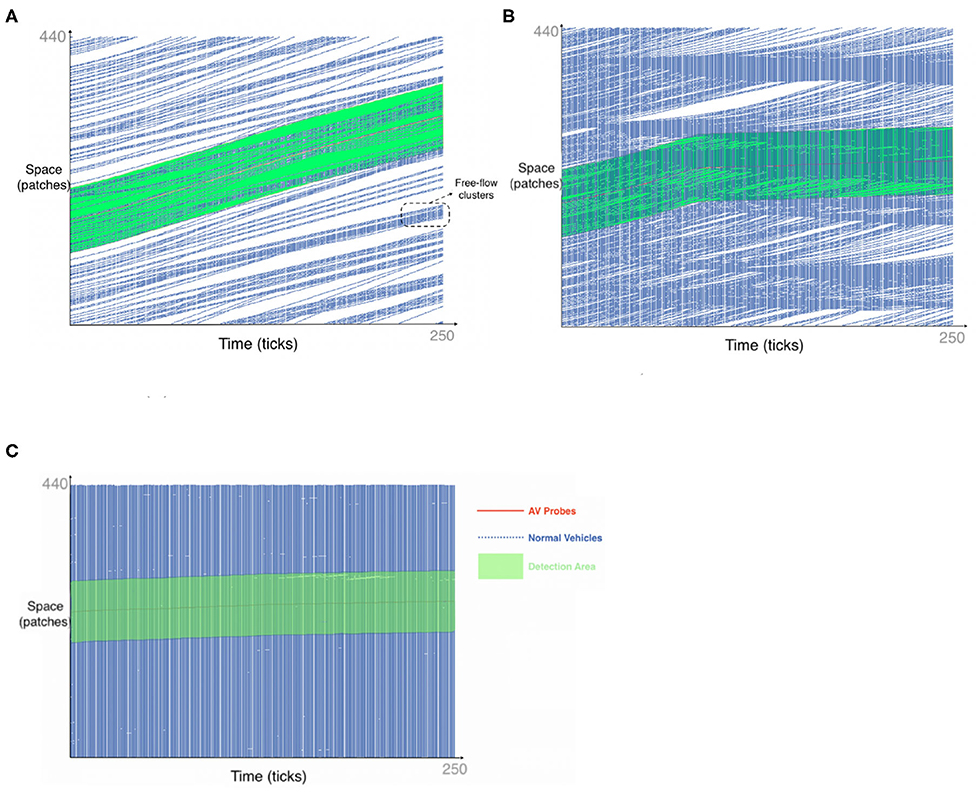
Figure 3. Time-space plot of single probe in one direction. (A) 10% road coverage. (B) 30% road coverage. (C) 70% road coverage.

FIGURE 4

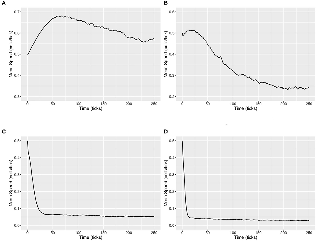
Figure 4. Speed maps for different traffic states. (A) Global mean speed map under 10% road coverage. (B) Global mean speed map under 30% road coverage. (C) Global mean speed map under 70% road coverage. (D) Global mean speed map under 90% road coverage.

To explore the probe errors in varying traffic conditions, a preliminary set of experiments was conducted at 10% intervals of road coverage, with five experiments of 5,000 timesteps for each traffic condition. The results did not follow a pure exponential but a double-hump trend. The unexpected nature of these results led to another set of experiments with the same conditions and sample sizes (20 times 5,000—timestep tests for each road coverage percentage in the detailed 0–30% range) in order to clarify the double-hump trend further. The double-hump curve was found to be consistent across both preliminary experiments.

The final experiment's results can be seen in Figure 5A. The magnitudes of the errors are comparable to most outcomes in other studies (Seo et al., 2015a; Fountoulakis et al., 2017) (presented in Table 2), with the difference in error trends caused by considering traffic heterogeneity and shockwaves. The results show high levels of absolute error for low road coverage, however this error quickly decreased as road coverage approached (approximately) 20%. Following this, there was a second jump back up to high levels of error, which decreased again, in an approximately exponential trend, as road coverage approached jam density.

FIGURE 5

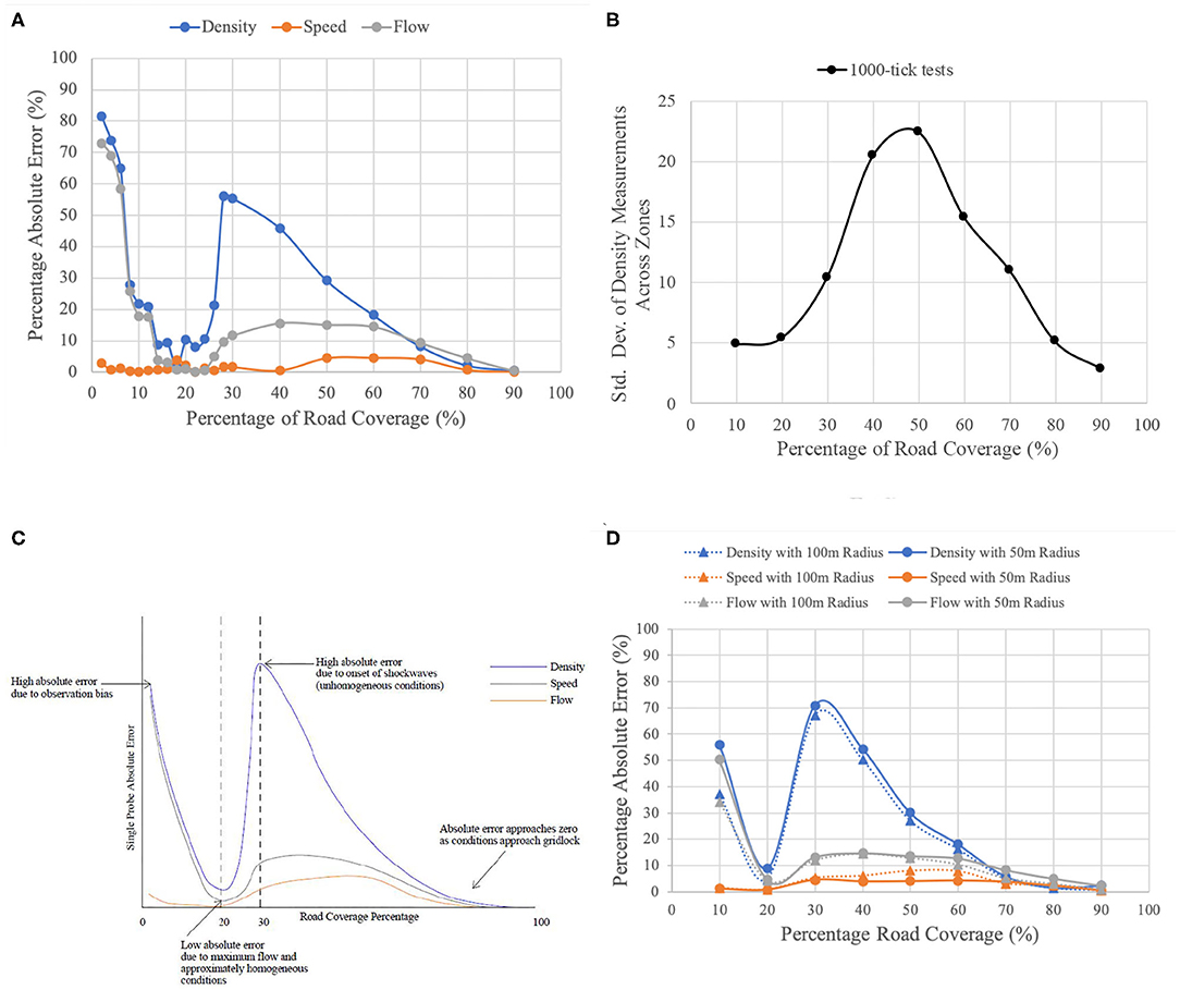
Figure 5. Double-hump trend of the single probe and explanation. (A) Single probe absolute error to road coverage. (B) Stochasticity in different road coverages. (C) Idealized double-hump curve. (D) Comparison of absolute error for ideal and reduced visibility radius.

TABLE 2

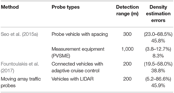
Table 2. Results comparison to other studies with varying AV penetration rates.

To attempt to explain this double-hump trend, further analysis that produces a more nuanced view of the changes in traffic conditions and how they affect error is required. Firstly, with the aim of establishing the density corresponding to the maximum flow in the model, a q-k curve was plotted based on the overall observer's measurements. It illustrated that maximum flow occurred at 20% road coverage. Therefore, it was suggested that the maximum flow point is correlated with the first decrease in error in the double hump curve, as this also occurs at 20% road coverage. The reason for this correlation is probably that at maximum flow, the probe is moving most efficiently with almost no shockwaves, and then it is getting a larger and more representative sample of vehicles along its trajectory.

Further to this, the traffic conditions were analyzed based on stochasticity. To measure stochasticity, 1,000-timestep tests were run for a range of road coverages. The standard deviations of the densities measured in each zone were plotted for varying coverage percentages. Thus, the variability of the different percentages along the pipeline were compared. The results are shown in Figure 5B.

From the above results, at the beginning, the errors are high, because the single probe is highly like to be within a platoon and observe the locally high density. Then, it reaches the point of maximum flow (around 20% road coverage), traffic conditions are relatively smooth, with nearly no shockwaves. For road coverage higher than 20%, it was observed during model simulations that stop-and-go waves had started occurring in the traffic, and then caused lower flow rates. When the flow rate is lowered, the accuracy benefits associated with high flow rates are removed. The stochasticity of the road conditions peaks at around 40–50% road coverage, but then sharply decreased as conditions approached jam density. Following the increase in error associated with the onset of shockwaves, the error was found to decrease as conditions approached jam density. This was in keeping with the hypothesis mentioned before. The double-hump absolute error trend for a single probe, and the major factors leading to it may therefore be approximately expressed in the idealized diagram in Figure 5C.

In both Figure 5A and its idealization Figure 5C, we found that the accuracy of flow was a function of the accuracy of density and the accuracy of speed measurements. It appears that density inaccuracy dominates flow inaccuracy up until 20% coverage. However, speed inaccuracy dominates flow inaccuracy for the rest. It is clear that density error is consistently much larger than speed error. This is expected given that density is subject to both traffic heterogeneity and shockwaves and is thus highly sensitive. Speed, on the other hand, is forgiving in that most vehicles are moving within a relatively small band of speeds, and thus any sample of speeds taken by the probe will not have a very large error.

For all the above tests, a radius of visibility of 22 cells (approximately 100 m) has been used for the probe in the model. This is the ideal visible range of current LIDAR technology. However, in reality it is likely that this ideal range would often not be possible due to obstacles and weather conditions (among other causes of visibility reduction). It is, however, hoped that improvements in technology and well-placed LIDAR sensors will allow the ideal visible radius to be largely met in reality. Nonetheless, a series of tests were run to assess the absolute error of a single probe with a reduced radius of visibility. The reduced radius was taken as 11 cells (approximately 50 m). The results of the reduced radius tests are shown below in Figure 5D. Note that for each percentage of road coverage, 10 tests of 5,000 timesteps were undertaken, so that the sample size is consistent with the ideal (22 cells) visibility radius data presented again.

From Figure 5D, it will be noticed that for both density and flow measurements, there is a consistent increase in the absolute error from the ideal visibility radius to the reduced visibility radius, which is generally not very significant except for low road coverage. However, for speed measurements, there is a large portion of road coverage percentages (30–70%) where the absolute error actually decreases with the reduced visibility radius. This feature, however, is caused by the reduced visibility radius that decreases the observation of shockwaves so that the accuracy slightly increases. Overall, the marginal increase in error (or the resulting additional error) associated with reduced visibility means that even in situations where LIDAR cannot be used to its full potential due to obstacles or weather, is not very significant. It should be noted that the conclusion above is on the premise that the probe recognizes when it is experiencing reduced visibility, then reduces its radius of visibility uniformly, and bases any density calculations off that smaller section of road.

To summarize, a single probe's absolute error follows a double-hump trend, with the high error associated with low road coverage; low error associated with the point of maximum flow; high error again associated with the onset of shockwaves; and low error again associated with the approach to jam density conditions. The reason is mainly because the probe's error is affected by heterogeneous traffic conditions with clusters in the relative low coverage regime and stop-and-go waves in the relative high coverage regime. Furthermore, even though a probe is generally less accurate than a comparable static induction loop detector in low road coverage situations or its visibility radius gets restricted, it still shows the potential of collecting the data efficiently and economically.

5.2. Multiple Probes in One-Directional Pipeline

The second scenario that was considered involved up to 100 probes in a three-lane one-directional pipeline which was identical to that used for Scenario 1. The aim of this scenario was to explore the reduction of error associated with multiple probes, and at what point the addition of probes no longer contributed meaningful error reduction. Again, this was tested under a range of traffic conditions by varying the road coverage percentage.

It had been originally hypothesized that an increase in the number of probes would decrease the absolute error associated with density, speed, and flow measurement. After the verification of simulation results, this was broadly found to be the case that the majority of the decrease in error was achieved by a relatively small number of additional probes, but with some unexpected “noise” in the data. Even when increasing number of probes, the common observation bias appears to be significant. The results measuring the percentage absolute error of parameters at 10, 20, 30, and 70% road coverage, for 1, 2, 10, 20, and 100 probes, are presented in Figures 6A–C. For each percentage of road coverage, five simulations were undertaken of 1,000-timestep length and the results averaged.

FIGURE 6

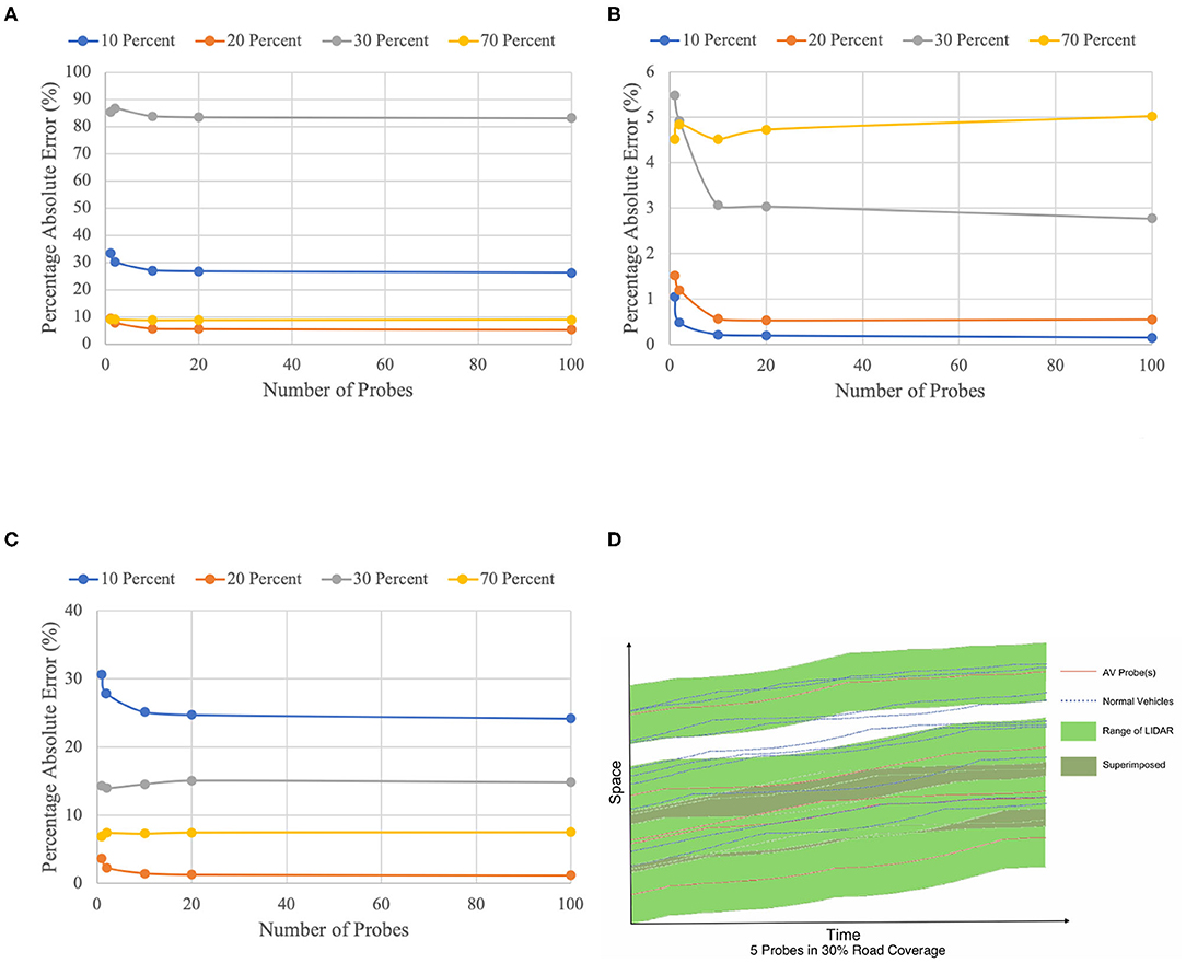
Figure 6. Percentage absolute error for multiple probes. (A) Percentage absolute error in density measurement. (B) Percentage absolute error in speed measurement. (C) Percentage absolute error in flow measurement. (D) Space-time plot of multiple probes in one direction.

From Figure 6A, it is clear that the reduction in error in the measurement of density between 10 probes and 100 probes is relatively small for all percentages of road coverage tested. Any additional probes to these are not contributing any substantial reduction of error. It is also found that the improvement due to additional probes becomes less significant progressively from 10% road coverage (with a reasonably steep improvement), to 70% road coverage (with practically no improvement).

The reduction of speed measurement error with the increase of probes from Figure 6B is generally similar to that of density. However, the errors are of a much smaller magnitude and in a much smaller range, which is the reason for a lot of noise in the data, and the apparently inexplicable trend at 70% road coverage. It is again clear that any more than 10 probes (5 probes per kilometer) will not deliver any substantial error reduction in speed measurement. Similarly, the trend registers the greatest improvement with the onset of shockwaves (around 20% road coverage).

Again the reduction of flow measurement error with the increase of probes is broadly consistent with density and speed shown in Figure 6C. Given that density measurement tends to dominate flow measurement, the flattening of the curves with increased road coverage is again apparent, though more noise is present due to the noise within both the density and the speed measurement data.

The small error reductions, even when there are large numbers of probes present, point to the considerable structural error associated with moving array probes. This structural error is mainly identified as common observation bias where most of the vehicles are probes. Because the multiple probes drive in the same direction, they “share” the observation bias as shown in the superimposed parts (filled by dark green) of Figure 6D with each other so that the bias cannot be eliminated progressively with increased percentage of probes, even when it reaches 100% probes. In this case, it is clear that there will be an overestimation of vehicle density due to the shared bias. However, unfortunately, this structural error is unavoidable, and it is the reason behind the relatively small error reductions associated with multiple probes.

Thus, it can be concluded that an increased number of probes reduces the absolute error associated with density, speed, and flow measurement, with an optimum of 10 probes. However, the reductions in error, as observed, are quite small due to the superimposed bias of multiple probes.

5.3. Single Probe in Two-Directional Pipeline

The third scenario that was considered involved a single probe in a six-lane, two-directional pipeline essentially a duplication of the pipeline used previously. From that, a further aspect of the probe's ability to measure the density, speed and flow of vehicles passing in the opposite direction is tested. Insofar as this scenario involves two directions of traffic, it better approximates reality.

With the model consistency being established, the probe's measurement error for the oncoming traffic's information was plotted and distinguished against the error associated with measuring concurrent traffic. The results are progressively presented below in Figures 7A–D. Note the x-axis (Percentage of Road Coverage) represents the varying traffic states for either direction of the road, depending on in which direction the errors are measured.

FIGURE 7

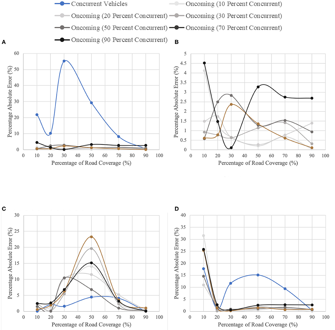
Figure 7. Percentage absolute error for a single probe in a two-directional pipeline. (A) Percentage absolute error in density measurement. (B) Percentage absolute error in density measurement (oncoming only). (C) Percentage absolute error in speed measurement. (D) Percentage absolute error in flow measurement.

Figure 7A shows that the error is consistently lower when the probe measures the density of oncoming traffic as opposed to concurrent traffic regardless of the concurrent varying road coverage. The reason for this significant reduction in error can be that the probe detects a much larger sample of different vehicles and conditions when viewing oncoming traffic. Moreover, a probe traveling in the opposite direction is not more likely to be within areas of congestion that would normally cause observation bias, so that aspect of observation bias is largely removed in the case of oncoming traffic. However, to investigate how the accuracy of oncoming traffic density measurement is affected by concurrent traffic conditions, these cases are enlarged in Figure 7B. From this figure, it is clear that the trends are quite opaque, given that the range in which these errors occur is 0–4.5%. Also, it may be seen that, broadly speaking, the lowest error occurs when the concurrent traffic conditions are at 20% road coverage, which is associated with the highest levels of flow, and thus with the largest sample possible (both of concurrent and oncoming traffic). Note that despite the noise in the data and the small range of errors, it may be assumed that concurrent traffic conditions have relatively little (and quite unpredictable) effects on the accuracy of density measurements of oncoming traffic.

From Figure 7C, there tends to be a single hump-like curve in error when measuring the speed of oncoming traffic, under all concurrent traffic conditions. That is because with the onset of shockwaves, a probe tends to see more slow-moving vehicles since it is more likely to be within a shockwave itself. Besides, when observing oncoming traffic, the probe tends to observe shockwaves for a longer time than areas of free-flow given their slower movement. Since the error is based on an average of all measurements (50,000—one corresponding to each timestep), a disproportionate number of the timesteps will have been spent observing shockwaves in the oncoming traffic. Thus, overall, slow-moving vehicles are over-represented when shockwaves occur so that it leads to the underestimation of the speed in road coverage percentages where shockwaves are present.

From Figure 7D, it can be seen that, again, flow measurement error tends to follow density more than speed. Thus, as for density, the measurement of flow has a (generally) substantial reduction in error when it is of the oncoming traffic rather than concurrent traffic. All the preceding reasons are applicable here since the flow is merely the product of density and speed. However, it is notable that the measurement of oncoming traffic appears to be sometimes less accurate than of concurrent traffic. This occurs when concurrent traffic is at 10% coverage due to associated with observation bias due to insufficient vehicles to detect, and when concurrent traffic is at high percentages (70–90), which reduces the sampling power of the probe due to its slow movement. Despite that, it is clear that in the measurement of flow, it is generally more accurate to measure oncoming traffic rather than concurrent traffic.

6. Conclusion

It has been seen that there is potential in the use of autonomous vehicles as moving array probes. Through the construction of three scenarios, the nature and trends in probe “error” have been detected, presenting the possibility of correction, which may produce results that are acceptable given the other benefits associated with AV probes and the conditions being monitored. Research should be directed to developing techniques to correct for measurement bias. The term “error” itself is a somewhat misleading, as the probe measures the world subjectively, from the point-of-view of the moving vehicle (as a moving array), while the objective loop detector is objective from a fixed point or in the case of complete coverage, all fixed points (providing the omniscient perspective). But the probe measurement, which is time-weighted, i.e., depends on how much time is spent in traffic, is actually closer to how travelers perceive traffic than how system managers measure it (Levinson, 2003), and may provide valuable insights by itself.

The most fundamental finding relating to a single probe's error was the double-hump trend. Probe error was thus found to be the result of an interaction between traffic heterogeneity and shockwaves. It was also found that when the probe's radius of visibility is reduced by half, the increase in error is small.

The results of the investigation into multiple probes differed slightly from expectations. It is found that while there is a decrease in error associated with an increase in the number of probes, it is generally not very large, or proportionate to the number of additional probes. The reason for this is the substantial and unavoidable structural observation bias and tendency to be within areas of congestion.

Finally, it was learned that the effects of concurrent traffic conditions on the observation of oncoming are appreciable but secondary. It was the case that high flow (critical density) in concurrent traffic, was broadly associated with the lower error in the measurement of oncoming traffic.

Future investigation can consider alternative geometric configurations beyond the pipeline including intersections and surrounding infrastructures. More scenarios (for instance, multiple probes in a two-directional pipeline) and more realistic traffic conditions may yield additional insights. Meanwhile, camera recordings are expected to be integrated with the LIDAR data for 3D scenes of tracking objects, which is ongoing in many autonomous vehicle companies. This technology will enhance not only self-driving technology but also the analysis of driver behavior. GPS and V2X communications systems may assist AV probes in the future. In situations where AV traffic is isolated, for instance in dedicated lanes, the accuracy of LIDAR data improves by reducing or eliminating the impact of platooning biases. Overall, it is hoped that this investigation has shown the potential and limitations of AVs used as moving array traffic probes, which is worthy of further research. While accuracy limitations were observed that differ from other traditional data collection methods, we believe these are correctable with appropriate calibration methods, and are outweighed by the economy and ubiquity that AV probes appear to offer.

Data Availability Statement

The original contributions presented in the study are included in the article/supplementary material, further inquiries can be directed to the corresponding author/s.

Author Contributions

BD: conceptualization, methodology, software, validation, and writing—original draft. AJ: software, validation, formal analysis, investigation, and writing—revised draft. BL: methodology, software, validation, and writing—original draft. DL: writing—review and editing and supervision. All authors contributed to the article and approved the submitted version.

Conflict of Interest

The authors declare that the research was conducted in the absence of any commercial or financial relationships that could be construed as a potential conflict of interest.

References

Antoniou, C., Balakrishna, R., and Koutsopoulos, H. N. (2011). A synthesis of emerging data collection technologies and their impact on traffic management applications. Eur. Trans. Res. Rev. 3, 139–148. doi: 10.1007/s12544-011-0058-1

CrossRef Full Text | Google Scholar

Bekiaris-Liberis, N., Roncoli, C., and Papageorgiou, M. (2016). Highway traffic state estimation with mixed connected and conventional vehicles. IEEE Trans. Intell. Transp. Syst. 17, 3484–3497. doi: 10.1109/TITS.2016.2552639

CrossRef Full Text | Google Scholar

Cao, M., Zhu, W., and Barth, M. (2011). “Mobile traffic surveillance system for dynamic roadway and vehicle traffic data integration,” in 2011 14th International IEEE Conference on Intelligent Transportation Systems (ITSC) (Washington, DC), 771–776. doi: 10.1109/ITSC.2011.6083096

CrossRef Full Text | Google Scholar

Carrese, S., Cipriani, E., Mannini, L., and Nigro, M. (2017). Dynamic demand estimation and prediction for traffic urban networks adopting new data sources. Transp. Res. Part C 81, 83–98. doi: 10.1016/j.trc.2017.05.013

CrossRef Full Text | Google Scholar

Cetin, M., Sazara, C., and Nezafat, R. V. (2017). Exploring the Use of Lidar Data From Autonomous Cars for Estimating Traffic Flow Parameters and Vehicle Trajectories. Technical report, Old Dominion University, Norfolk, VA.

Google Scholar

Chen, B., Yang, Z., Huang, S., Du, X., Cui, Z., Bhimani, J., et al. (2017). “Cyber-physical system enabled nearby traffic flow modelling for autonomous vehicles,” in Performance Computing and Communications Conference (IPCCC), 2017 IEEE 36th International (San Diego, CA), 1–6. doi: 10.1109/PCCC.2017.8280498

CrossRef Full Text | Google Scholar

Chen, C., Kwon, J., Rice, J., Skabardonis, A., and Varaiya, P. (2003). Detecting errors and imputing missing data for single-loop surveillance systems. Transp. Res. Rec. 1855, 160–167. doi: 10.3141/1855-20

CrossRef Full Text | Google Scholar

Coifman, B. (2003). Estimating density and lane inflow on a freeway segment. Transp. Res. Part A 37, 689–701. doi: 10.1016/S0965-8564(03)00025-9

CrossRef Full Text | Google Scholar

Coifman, B., Wu, M., Redmill, K., and Thornton, D. A. (2016). Collecting ambient vehicle trajectories from an instrumented probe vehicle. Transp. Res. Part C 72, 254–271. doi: 10.1016/j.trc.2016.09.001

CrossRef Full Text | Google Scholar

Cremer, M. (1991). “Flow variables: estimation,” in Concise Encyclopedia of Traffic & Transportation Systems, ed M. Papageorgiou (Pergamon: Elsevier), 143–148. doi: 10.1016/B978-0-08-036203-8.50035-3

PubMed Abstract | CrossRef Full Text

Davidson, P., and Spinoulas, A. (2015). “Autonomous vehicles: what could this mean for the future of transport,” in Proceedings of the Australian Institute of Traffic Planning and Management (AITPM) National Conference (Brisbane, QLD).

Google Scholar

Edie, L. C. (1963). Discussion of Traffic Stream Measurements and Definitions. Port of New York Authority.

Fagnant, D. J., and Kockelman, K. (2015). Preparing a nation for autonomous vehicles: Opportunities, barriers and policy recommendations. Transp. Res. Part A 77, 167–181. doi: 10.1016/j.tra.2015.04.003

CrossRef Full Text | Google Scholar

Fountoulakis, M., Bekiaris-Liberis, N., Roncoli, C., Papamichail, I., and Papageorgiou, M. (2017). Highway traffic state estimation with mixed connected and conventional vehicles: microscopic simulation-based testing. Transp. Res. Part C 78, 13–33. doi: 10.1016/j.trc.2017.02.015

CrossRef Full Text | Google Scholar

He, Z., and Zheng, L. (2017). Visualizing traffic dynamics based on floating car data. J. Transp. Eng. Part A 143:04017005. doi: 10.1061/JTEPBS.0000024

CrossRef Full Text | Google Scholar

Herrera, J. C., and Bayen, A. M. (2010). Incorporation of Lagrangian measurements in freeway traffic state estimation. Transp. Res. Part B 44, 460–481. doi: 10.1016/j.trb.2009.10.005

CrossRef Full Text | Google Scholar

Jenelius, E., and Koutsopoulos, H. N. (2015). Probe vehicle data sampled by time or space: consistent travel time allocation and estimation. Transp. Res. Part B 71, 120–137. doi: 10.1016/j.trb.2014.10.008

CrossRef Full Text | Google Scholar

Korosec, K. (2018). Waymo?s Self-Driving Cars Hit 10 Million Miles. TechCrunch.

Leduc, G. (2008). “Road traffic data: collection methods and applications,” in Working Papers on Energy, Transport and Climate Change.

Google Scholar

Leutzbach, W. (1988). Introduction to the Theory of Traffic Flow, Vol. 47. Berlin; Heidelberg: Springer-Verlag. doi: 10.1007/978-3-642-61353-1

CrossRef Full Text | Google Scholar

Levinson, D. (2003). Perspectives on efficiency in transportation. Int. J. Transp. Manage. 1, 145–155. doi: 10.1016/j.ijtm.2004.01.002

CrossRef Full Text | Google Scholar

Levinson, D. M., and Krizek, K. J. (2017). The End of Traffic & the Future of Access. Network Design Lab.

PubMed Abstract | Google Scholar

Lin, Y., Dai, X., Li, L., and Wang, F.-Y. (2018). Pattern sensitive prediction of traffic flow based on generative adversarial framework. IEEE Trans. Intell. Transp. Syst. 20, 2395–2400. doi: 10.1109/TITS.2018.2857224

CrossRef Full Text | Google Scholar

Liu, Y., Guo, J., Taplin, J., and Wang, Y. (2017). Characteristic analysis of mixed traffic flow of regular and autonomous vehicles using cellular automata. J. Adv. Transp. 2017:8142074. doi: 10.1155/2017/8142074

CrossRef Full Text | Google Scholar

Lou, Y., Li, P., and Hong, X. (2016). A distributed framework for network-wide traffic monitoring and platoon information aggregation using V2V communications. Transp. Res. Part C 69, 356–374. doi: 10.1016/j.trc.2016.06.003

CrossRef Full Text | Google Scholar

Ma, X., and Andréasson, I. (2006). Estimation of driver reaction time from car-following data: application in evaluation of general motor-type model. Transp. Res. Rec. 1965, 130–141. doi: 10.1177/0361198106196500114

CrossRef Full Text | Google Scholar

Makigami, Y., Newell, G. F., and Rothery, R. (1971). Three-dimensional representation of traffic flow. Transp. Sci. 5, 302–313. doi: 10.1287/trsc.5.3.302

CrossRef Full Text | Google Scholar

Morando, M. M., Tian, Q., Truong, L. T., and Vu, H. L. (2018). Studying the safety impact of autonomous vehicles using simulation-based surrogate safety measures. J. Adv. Transp. 2018:6135183. doi: 10.1155/2018/6135183

CrossRef Full Text | Google Scholar

Nanthawichit, C., Nakatsuji, T., and Suzuki, H. (2003). Application of probe-vehicle data for real-time traffic-state estimation and short-term travel-time prediction on a freeway. Transp. Res. Rec. 1855, 49–59. doi: 10.3141/1855-06

CrossRef Full Text | Google Scholar

Qiu, T. Z., Lu, X.-Y., Chow, A. H., and Shladover, S. E. (2010). Estimation of freeway traffic density with loop detector and probe vehicle data. Transp. Res. Rec. 2178, 21–29. doi: 10.3141/2178-03

PubMed Abstract | CrossRef Full Text | Google Scholar

Rahmani, M., Jenelius, E., and Koutsopoulos, H. N. (2015). Non-parametric estimation of route travel time distributions from low-frequency floating car data. Transp. Res. Part C 58, 343–362. doi: 10.1016/j.trc.2015.01.015

CrossRef Full Text | Google Scholar

Sanguesa, J. A., Barrachina, J., Fogue, M., Garrido, P., Martinez, F. J., Cano, J.-C., et al. (2015). Sensing traffic density combining V2V and V2I wireless communications. Sensors 15, 31794–31810. doi: 10.3390/s151229889

PubMed Abstract | CrossRef Full Text | Google Scholar

Schaub, A. (2018). Robust Perception from Optical Sensors for Reactive Behaviors in Autonomous Robotic Vehicles. Wiesbaden: Springer. doi: 10.1007/978-3-658-19087-3

CrossRef Full Text | Google Scholar

Schorr, J., Hamdar, S. H., and Silverstein, C. (2017). Measuring the safety impact of road infrastructure systems on driver behavior: vehicle instrumentation and real world driving experiment. J. Intell. Transp. Syst. 21, 364–374. doi: 10.1080/15472450.2016.1198699

CrossRef Full Text | Google Scholar

Seo, T., Bayen, A. M., Kusakabe, T., and Asakura, Y. (2017). Traffic state estimation on highway: a comprehensive survey. Annu. Rev. Control 43, 128–151. doi: 10.1016/j.arcontrol.2017.03.005

CrossRef Full Text | Google Scholar

Seo, T., Kusakabe, T., and Asakura, Y. (2015b). Estimation of flow and density using probe vehicles with spacing measurement equipment. Transp. Res. Part C 53, 134–150. doi: 10.1016/j.trc.2015.01.033

CrossRef Full Text | Google Scholar

Seo, T., and Kusakabe, Takahiko, and Asakura, Y. (2015a). “Traffic state estimation with the advanced probe vehicles using data assimilation,” in 2015 18th International IEEE Conference on Intelligent Transportation Systems (ITSC) (Las Palmas de Gran Canaria). doi: 10.1109/ITSC.2015.139

CrossRef Full Text | Google Scholar

Soria, I., Elefteriadou, L., and Kondyli, A. (2014). Assessment of car-following models by driver type and under different traffic, weather conditions using data from an instrumented vehicle. Simul. Model. Pract. Theory 40, 208–220. doi: 10.1016/j.simpat.2013.10.002

CrossRef Full Text | Google Scholar

van Erp, P. B., Knoop, V. L., and Hoogendoorn, S. P. (2018). Macroscopic traffic state estimation using relative flows from stationary and moving observers. Transp. Res. Part B 114, 281–299. doi: 10.1016/j.trb.2018.06.005

CrossRef Full Text | Google Scholar

Wang, Y., and Papageorgiou, M. (2005). Real-time freeway traffic state estimation based on extended Kalman filter: a general approach. Transp. Res. Part B 39, 141–167. doi: 10.1016/j.trb.2004.03.003

CrossRef Full Text | Google Scholar

Wilensky, U. et al. (1998). “Netlogo traffic 2 lanes model,” in Netlogo (Center for Connected Learning and Computer-Based Modeling; Northwestern University).

Work, D. B., Blandin, S., Tossavainen, O.-P., Piccoli, B., and Bayen, A. M. (2010). A traffic model for velocity data assimilation. Appl. Math. Res. Exp. 2010, 1–35. doi: 10.1093/amrx/abq002

CrossRef Full Text | Google Scholar

Xu, D., Wei, C., Peng, P., Xuan, Q., and Guo, H. (2020). GE-GAN: A novel deep learning framework for road traffic state estimation. Transp. Res. Part C 117:102635. doi: 10.1016/j.trc.2020.102635

CrossRef Full Text | Google Scholar

Xuan, Y., and Coifman, B. (2012). Identifying lane-change maneuvers with probe vehicle data and an observed asymmetry in driver accommodation. J. Transp. Eng. 138, 1051–1061. doi: 10.1061/(ASCE)TE.1943-5436.0000401

CrossRef Full Text | Google Scholar