Dynamics of Flow Merging and Diverging in MFD-Based Systems: Validation vs. Microsimulation

1. Introduction

1.1. Research Question

Since the early works of Daganzo (2007) and Geroliminis and Daganzo (2007), using the Macroscopic Fundamental Diagram (MFD) to simulate traffic states at the city scale has attracted increasing interest in the literature. In particular, numerous studies (see e.g., Keyvan-Ekbatani et al., 2012, 2015; Kouvelas et al., 2017; Zhong et al., 2018; Sirmatel and Geroliminis, 2019; Haddad and Mirkin, 2020) have used MFD-based simulation to design promising traffic control frameworks for large-scale networks, where such networks are split into several homogeneous reservoirs (urban areas) with a well-defined MFD. However, there is still a lack in understanding flow exchanges and limitations at the reservoir boundaries in multi-reservoir systems. More precisely, we identify three research questions that need to be investigated: (i) How can the maximum available flow that can enter a reservoir, for both under- and over-saturated conditions be defined dynamically? (ii) How can inflow merging be managed? and (iii) How can outflow diverging be managed when different demand flows are distinguished (by their origins, destinations, or regional paths)?

1.2. Literature Review

The literature provides no complete response to any of these questions. The first refers to what is sometimes called the “entry supply function” of the reservoir (also named “receiving capacity” or “boundary capacity”). It is assumed to be a decreasing function of the reservoir accumulation and represents the total available inflow entering the reservoir. Its value is maximum when the accumulation is small (under-saturation), and goes down to zero when the accumulation is high (over-saturation). Its existence has been shown by Geroliminis and Daganzo (2007) through a simulation study. Other authors like Hajiahmadi et al. (2013), Knoop and Hoogendoorn (2014), Lentzakis et al. (2016), and Mariotte and Leclercq (2019) adopted an entry supply function with a shape based on the Cell Transmission Model (CTM) of Daganzo (1994). The reason behind this approach is that the theoretical formulation of the reservoir dynamics may correspond to cell dynamics in the CTM. Thus, connecting together a sequence of reservoirs would be similar to connecting a sequence of cells. This solution is appealing as we know from kinematic wave theory that such a formulation efficiently reproduces congestion propagation between entities. However, the objection to this approach is that the cell properties cannot be scaled up at the reservoir level. In particular, the maximum inflow capacity and the critical accumulation (at which the inflow capacity starts decreasing) of the entry supply function may differ from the MFD's capacity and critical accumulation. For instance, Geroliminis and Daganzo (2007) showed with their simulation results that the critical accumulation of the supply function is double that of the critical accumulation of the MFD. Aboudolas and Geroliminis (2013) was the first to propose an MFD-based traffic management strategy with a multi-reservoir settings using microsimulation tests on San Francisco network. However, the authors did not use inflow or outflow functions to manage the boundary flows. In Ramezani et al. (2015) and Sirmatel and Geroliminis (2017), a simple piecewise linear function was used with these two parameters (the maximum inflow capacity and the critical accumulation). This was also probably the approach taken by Yildirimoglu and Geroliminis (2014) and Yildirimoglu et al. (2015), although not explicitly mentioned in their works. Interestingly, these authors designed a supply function for each reservoir boundary (thus each function limits inflow from a specific neighboring reservoir), but they did not provide further details about the interactions between these functions. Their implementation was merely justified by technical reasons, i.e., avoiding gridlocks in some scenarios, and the authors acknowledged the fact that their shapes would have negligible influence on their simulation results due to the action of perimeter control or route guidance. This was notably illustrated by Sirmatel and Geroliminis (2017), who performed a sensitivity analysis on the two function parameters they used and showed that these parameters had little impact on their study. These works inspired Mariotte and Leclercq (2019), who further discussed and illustrated the implications of such shapes of entry supply functions on MFD dynamics. In the stated work, the authors proposed the so-called endogenous entry flow function, which is different from the one widely used in the literature. It was also concluded that the conventional outflow model used in the literature results in unrealistic gridlock situations in over saturated traffic states. Lately, Kim et al. (2018) explored flow exchanges between reservoirs with the results from a micro-simulation, and proposed an even simpler shape for this function (linearly decreasing), also used in Zhang et al. (2015). Nevertheless, only inflow and outflow shares were tested with network loading scenarios, and the proposed entry supply function was not implemented in an MFD-based simulation. Haddad (2017) proposed a perimeter control strategy based on MFD by including the effect of boundary queues. Having the queued vehicles inside the reservoir due to outflow restrictions can influence the shape of MFD and consequently, the exit flow function. However, this effect of boundary queues is neglected and a well-defined MFD is assumed to exist at all times in the present work.

The second problem about inflow allocation is often solved by using merging rules based on demand pro-rata (see e.g., Geroliminis, 2009; Knoop and Hoogendoorn, 2014; Yildirimoglu and Geroliminis, 2014; Ramezani et al., 2015), or less often fair merging rules (see e.g., Zhong et al., 2018). Ge and Fukuda (2019) developed a unified merge and diverge model similar to Jin and Zhang (2004) to determine turning fractions in their multi-reservoir modeling, which is also based on demand pro-rata rules. On the other hand, Mariotte and Leclercq (2019) found that incorporating constraints on production into the merging scheme potentially leads to a different flow allocation. In this case, the inflow share at entry would also depend on the reservoir inner dynamics (i.e., evolution of each partial accumulation) and the different trip lengths inside the reservoir.

Finally, the third question on outflow diverging is rarely investigated in the literature. To the author's best knowledge, almost all studies on MFD-based modeling assume a decreasing reservoir outflow in over-saturated conditions. However, by reproducing the effect of reservoir internal congestion, and through simulation and empirical studies, Mariotte et al. (2017) and Mariotte and Leclercq (2019), showed that this assumption might lead to inefficient modeling of congestion propagation between reservoirs. They particularly insisted on the fact that the outflow demand of transferring trips that aim to enter a neighboring reservoir must be maximum in congestion, which is what would be observed on a simple network like an arterial. Recently, Wada et al. (2019) derived an analytical method to track congestion patterns and spillbacks in networks by solving an inverse Dynamic User Equilibrium (DUE) problem. Their method provided an analytical formulation of the network throughput, validated with link-level simulation. They showed that the network exit flow remains constant in over-saturated conditions for simple configurations, but decreases for more complex grid networks where users have many different destinations.

It is worth noting that the multi-reservoir models that are being investigated in the current work aim to provide traffic predictions over a medium to large time horizon for the systems that do not necessarily have active perimeter control. Such a case requires advanced modeling of congestion spillbacks. Most Model Predictive Control (MPC) approaches use short (about a few seconds) time horizons, which essentially reduces discrepancies due to inaccurate predictions. Furthermore, perimeter control aims to avoid congestion spillbacks as the reservoir operates at the peak capacity. So, a simple MFD model formulation without use of entry and exit flow functions is certainly sufficient. The ability of simpler MFD formulations for control application have already been tested when the time horizon is increased to 1 or 2 min. In other words, accumulations from the plant model are only updated every 1 or 2 min. We found that such a formulation failed to provide proper predictions, which significantly deteriorated the control performances (Batista et al., 2020). This limitation highlights the need for more advanced formulations if longer time horizons are used for predictions.

1.3. Objective and Methodology

In this work, we want to further investigate these three questions by comparing different assumptions in MFD-based approaches with microsimulation outputs. Without loss of generality and to simplify the settings, we focus on a single reservoir with multiple flows. Doing a similar study in the multi-reservoir settings will not change the conclusions. For instance, the entry flow function is only relevant at the external node, where inflow demand is imposed from outside the network. Suppose a reservoir is present between two reservoirs in a multi-reservoir setting. In that case, the inflow to the given reservoir is simply the outflow of the upstream reservoir and similarly, the outflow is the inflow capacity of the upstream reservoir. Thus, the flow dynamics are relevant only if the entries and exits are external in the present context. That is we choose a single reservoir setting to present the results with more clarity and ease. Moreover, we already presented a validation study (Mariotte et al., 2020) using a multi-reservoir MFD framework on a real network using empirical demand and OD matrix data. Our case study consists of a regular grid network crossed by two main regional flows (West-East and North-South). On the one hand, network-level traffic states on each regional flow (accumulation, inflow, outflow, production) are estimated by aggregating the link-level outputs from the microsimulation. These states are assumed to represent the ground truth of the grid network traffic dynamics. On the other hand, aggregated traffic states are simulated with an MFD accumulation-based model including multiple trips, so that each regional flow is represented by a partial accumulation, inflow and outflow. Two different representations of traffic dynamics exist in the literature, namely accumulation-based and trip-based models, see Mariotte et al. (2017) for an extensive review. As we will focus on highly congested situations in this study, we use only the accumulation-based approach and not the trip-based one, as the latter was found to behave similarly to the accumulation-based model in such situations (Mariotte and Leclercq, 2019). At the network entry, two inflow merging schemes are tested against the microsimulation results: (i) demand pro-rata merging, depending on the ratio of external demands that want to enter the reservoir (commonly used in the literature); and (ii) endogenous merging, depending on the ratio of partial accumulation inside the reservoir (see Mariotte and Leclercq, 2019). Also tested at the network exit are two outflow diverging schemes based on (i) a decreasing outflow demand in oversaturation (widely used in the literature), and (ii) based on a maximum outflow demand in oversaturation (our approach). We particularly focus on steady-state predictions of network loading scenarios, where congestion is created by fixing exogenous flow limitation at the network exit links. This is the most stressful situation for MFD models, as oversaturation is discussed less in the literature. The network MFD is calibrated using stationary network loadings with microsimulation. Our results first allow the calibration of a reliable entry supply function for the network studied, and second, the comparison between the above-mentioned inflow merging and outflow diverging models.

This paper takes the following structure: first, the different MFD-based modeling approaches to be compared are introduced; second, the simulation case study is presented; and finally, the microsimulation results are analyzed and compared with the different MFD models.

2. Multiple Trips in the Single Reservoir Model: Review of Existing Approaches

In this section, we present the main approaches that have been developed in the literature to describe flow exchanges in a single reservoir with multiple trip categories. We particularly focus on the underlying flow merge and diverge models that characterize these approaches.

2.1. General Framework

We consider an urban area described by a single reservoir model (Daganzo, 2007; Geroliminis and Daganzo, 2007), i.e., where traffic states are represented by a well-defined production-MFD P(n) (in [veh.m/s]) or speed-MFD V(n) = P(n)/n (in [m/s]), n(t) (in [veh]) being the total accumulation (number of vehicles traveling in the reservoir at time t). The production-MFD is defined by: the jam accumulation n_j and the critical accumulation n_c where the production reaches its maximum P_c = P(n_c). We investigate flow exchanges in the framework of multiple trip categories, as first introduced in Geroliminis (2009, 2015) and further used in Yildirimoglu and Geroliminis (2014), Ramezani et al. (2015), Haddad (2015), and Mariotte et al. (2020). We use these different approaches from the literature as presented and synthesized in Mariotte and Leclercq (2019). In this study, a trip category defines a “macroscopic route” (sometimes called “regional path”) or simply “route” in the following. It corresponds to the aggregation of multiple individual paths on the real street network that shares certain common characteristics (e.g., similar topology or length, following the same sequence of reservoirs in multi-reservoir systems, etc.). It usually has its own length, which requires considering multiple trip lengths in each reservoir (see also Batista et al., 2019; Paipuri et al., 2020).

Let us assume that the single reservoir considered comprises N routes with lengths {L_i}_1≤i≤N and corresponding accumulations {n_i(t)}_1≤i≤N, the total accumulation being $n(t)=\sum _{i=1}^N{n}_i(t)$. The system dynamics are described by the following conservation equations (Geroliminis, 2015):

$\begin{array}{ll}\forall i\in \left\{1,\dots ,N\right\},\frac{d{n}_i}{dt}=q_{\text{in},i}(t)-q_{\text{out},i}(t)& (1)\end{array}$

where q_in,i(t) and q_out,i(t) are route i effective inflow and outflow, respectively. These flow values therefore govern the entire evolution of the system, and are the result of the entry supply and merging and diverging schemes that are presented next. The general configuration of the reservoir exchanging flows with its neighbors is summarized in Figure 1. As in Mariotte and Leclercq (2019), we distinguish the routes by the location of their origin and destination (inside or outside the reservoir) for the treatment of their inflow and outflow. From the reservoir point of view, each route i has an exogenous demand λ_i(t) at its entry, which represents the flow sent from another reservoir or generated inside. It also has an exogenous supply μ_i(t) at its exit, which represents limitations to enter the next reservoir or possible constraints to park inside.

FIGURE 1

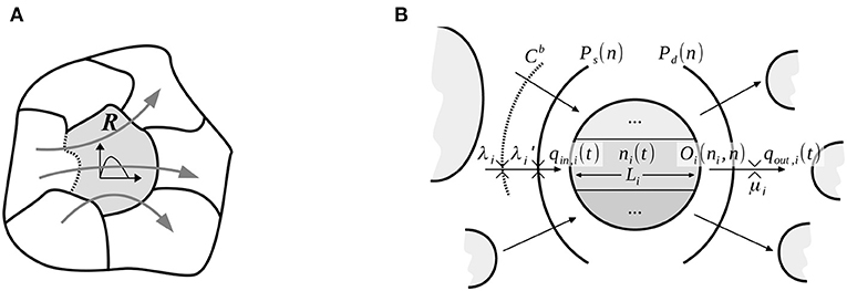
Figure 1. Single reservoi configuration crossed by multiple routes, (A) multi-reservoir context where one of the reservoir borders is represented by a dashed line, and (B) detail of flow exchanges on a given route.

2.2. Reservoir Exit Demand and Outflow Diverging Scheme

As in Mariotte and Leclercq (2019), the routes that end inside the reservoir (defined by the set ${{P}}_{\text{out}}^{\text{int}}$) are considered unconstrained at exit for simplicity:

$\begin{array}{ll}\forall i\in {{P}}_{\text{out}}^{\text{int}},{\mu }_i(t)=+\infty & (2)\end{array}$

On the contrary, the routes that end outside the reservoir (defined by the set ${{P}}_{\text{out}}^{\text{ext}}$) have their outflow possibly limited by capacity constraints from downstream reservoirs. This outflow is calculated as the confrontation between demand and supply at exit. The outlow demand corresponds to (Geroliminis, 2015; Mariotte and Leclercq, 2019):

$\begin{array}{ll}\forall i\in {{P}}_{\text{out}}^{\text{ext}},O_i(n_i,n)=\frac{n_i}{n}\frac{P_d(n)}{L_i}(\text{outflow demand})& (3)\end{array}$

where P_d(n) is called the exit production demand. The meaning of this concept is more mathematical than physical, it was first mentioned in Mariotte and Leclercq (2019) to ease the presentation of the different outflow models. It is directly defined from the production-MFD P(n). In the literature, the most widely used model is simply (Yildirimoglu and Geroliminis, 2014; Geroliminis, 2015):

$\begin{array}{ll}{P}_d(n)=P(n)\left(\text{decreasing exit demand}\right)& (4)\end{array}$

However, Mariotte et al. (2017) and Mariotte and Leclercq (2019) proposed a different formulation to better reproduce congestion dynamics:

$\begin{array}{ll}{P}_d(n)=\{\begin{array}{ll}P(n)& \text{if }n<n_c\\ P_c& \text{otherwise}\end{array}(\text{maximum exit demand})& (5)\end{array}$

As shown by the same authors, these formulations have a direct implication on the definition of the outflow diverge model. For the decreasing exit demand model, the effective outflows are calculated as (Yildirimoglu and Geroliminis, 2014):

$\begin{array}{ll}\{\begin{array}{ll}\forall i\in {{P}}_{\text{out}}^{\text{ext}},& q_{\text{out},i}(t)=min\left[{\mu }_i(t);O_i(n_i,n)\right]\\ \forall i\in {{P}}_{\text{out}}^{\text{int}},& q_{\text{out},i}(t)=\frac{n_i(t)}{n(t)}\frac{P(n)}{L_i}\end{array}(\text{for decreasing exit dem}.)& (6)\end{array}$

As for the maximum exit demand model, the effective outflows are obtained as follows (Mariotte and Leclercq, 2019):

$\begin{array}{ll}{q}_{\text{out},k}(t)=min\left[{\mu }_k(t);O_k(n_k,n)\right]\left(\text{most constrained outflow}\right)& (7)\end{array}$

$\begin{array}{l}\text{where: }k=\text{arg}{\displaystyle \underset{1\le i\le N}{min}}\frac{{\mu }_i}{O_i(n_i,n)}\\ \forall i\in \left\{1,\dots ,N\right\},i\ne k,\\ q_{\text{out},i}(t)=\frac{n_i(t)}{n_k(t)}\frac{L_k}{L_i}{q}_{\text{out},k}(t)(\text{for maximum exit dem}.)& (8)\end{array}$

The reader can refer to the discussion in Mariotte and Leclercq (2019) for the justification of this new outflow diverge model. In brief, decreasing exit diverge formulation might result in unrealistic gridlock scenarios when reservoir becomes oversaturated. In other words, network cannot recover from the congestion once it goes into oversaturation even if the demand is reduced. On the other hand, the so-called maximum exit diverge model can address this limitation.

In the following, these two diverge models are named after the underlying exit demand model. They are thus referred to as “decreasing exit diverge” and “maximum exit diverge” models.

2.3. Reservoir Entry Supply and Inflow Merging Scheme

As in Mariotte and Leclercq (2019), the routes that originate inside the reservoir (defined by the set ${{P}}_{\text{in}}^{\text{int}}$) are assumed to be unconstrained at entry:

$\begin{array}{ll}\forall i\in {{P}}_{\text{in}}^{\text{int}},q_{\text{in},i}(t)={\lambda }_i(t)& (9)\end{array}$

On the contrary, the routes that originate outside the reservoir (defined by the set ${{P}}_{\text{in}}^{\text{ext}}$) have their inflow possibly limited by capacity constraints from the reservoir. As detailed in Mariotte and Leclercq (2019) and Mariotte et al. (2020), these inflow restrictions have two origins. First, an exogenous one that comes from the physical capacity of all the links at a specific border of the reservoir (links connected to a specific neighboring reservoir). If we assume that the reservoir has N_B borders (i.e., common boundaries with neighboring reservoirs), each capacity C^b (1 ≤ b ≤ N_B) is expressed as the sum of all the flow capacity of links in border b (in [veh/s], including traffic signal settings of extremity node intersections). Second, the other inflow restriction is endogenous as it comes from the inner congestion state of the reservoir. It is defined with the entry supply function P_s(n), which concept and possible shapes were discussed in Mariotte and Leclercq (2019). Like these authors, we define it in production units and consider its modified expression $P_s^{\text{ext}}(n)=P_s(n)-\sum _{i\in {{P}}_{\text{in}}^{\text{int}}}{L}_i{\lambda }_i$ due to the presence of internal trips (routes in ${{P}}_{\text{in}}^{\text{int}}$). It is converted into flow units as $P_s^{\text{ext}}(n)/L^{\text{ext}}$ thanks to the dynamic average trip length of the routes in ${{P}}_{\text{in}}^{\text{ext}}$: $L^{\text{ext}}=\sum _{i\in {{P}}_{\text{in}}^{\text{ext}}}{n}_i/\sum _{i\in {{P}}_{\text{in}}^{\text{ext}}}\frac{n_i}{L_i}$ (Mariotte and Leclercq, 2019). The validation and calibration of this entry supply function will be investigated in section 4.1.

Then, these capacity constraints are allocated to each entering route i with a merge coefficient α_i(t), providing that $\sum _{i=1}^N{\alpha }_i(t)=1$. Thus, different inflow merge models are derived from the definition of these coefficients. As described in the introduction, to the authors' best knowledge the merge coefficients α_i are almost always assumed to correspond to demand pro-rata (see e.g., Geroliminis, 2009; Knoop and Hoogendoorn, 2014; Yildirimoglu and Geroliminis, 2014; Ramezani et al., 2015):

$\begin{array}{l}\forall i\in {{P}}_{\text{in}}^{\text{ext}},\\ {\alpha }_i(t)=\frac{{\lambda }_i(t)}{{\displaystyle {\sum }_{j\in {{P}}_{\text{in}}^{\text{ext}}}}{\lambda }_j(t)}(\text{demand pro-rata coefficients})& (10)\end{array}$

On the other hand, Mariotte and Leclercq (2019) proposed these coefficients as defined endogenously by the reservoir state:

$\begin{array}{ll}\forall i\in {{P}}_{\text{in}}^{\text{ext}},{\alpha }_i(t)=\frac{n_i(t)}{{\displaystyle {\sum }_{j\in {{P}}_{\text{in}}^{\text{ext}}}}{n}_j(t)}(\text{endogenous coefficients})& (11)\end{array}$

Aside from this, a new allocation scheme was proposed in Paipuri and Leclercq (2020). It is based on a First-In-First-Out (FIFO) rule and thus does not require merging coefficients. We also include it in this study for comparison.

As in Mariotte et al. (2020), the two sources of inflow limitation are combined in a two-layer merging scheme, as illustrated in Figure 1B. The first layer applies the border flow restrictions to the original demands λ_i, while the second layer takes the restricted demands ${\lambda }_i^{\prime }$ as inputs and applies the reservoir supply $P_s^{\text{ext}}(n)$ to them. For any given merge coefficients, the first layer always consists of a flow merge. On the other hand, the second layer is either: (i) a flow merge when using demand pro-rata coefficients [with available capacity $P_s^{\text{ext}}(n)/L^{\text{ext}}$]; or (ii) a production merge when using endogenous coefficients [with available capacity $P_s^{\text{ext}}(n)$]; or (iii) the FIFO rule from Paipuri and Leclercq (2020). This two-layer scheme is described as follows (Mariotte et al., 2020):

$\begin{array}{c}\forall b\in \left\{1,\dots ,N_B\right\},\\ {\left\{{\lambda }_i^{\prime }\right\}}_{i\in {{P}}^b}=\text{Merge}\left({\left\{{\lambda }_i\right\}}_{i\in {{P}}^b},{\left\{\frac{{\alpha }_i}{{\displaystyle {\sum }_{j\in {{P}}^b}}{\alpha }_j}\right\}}_{i\in {{P}}^b},C^b\right)& (12)\end{array}$

$\begin{array}{ll}\{\begin{array}{ll}{\{q_{\text{in},i}\}}_{i\in {{P}}_{\text{in}}^{\text{ext}}}=\text{Merge}\left({\{{\lambda }_i^{\prime }\}}_{i\in {{P}}_{\text{in}}^{\text{ext}}},{\{{\alpha }_i\}}_{i\in {{P}}_{\text{in}}^{\text{ext}}},\frac{P_s^{\text{ext}}(n)}{L^{\text{ext}}}\right)& \text{for demand pro-rata coeff}.\\ {\{L_i{q}_{\text{in},i}\}}_{i\in {{P}}_{\text{in}}^{\text{ext}}}=\text{Merge}\left({\{L_i{\lambda }_i^{\prime }\}}_{i\in {{P}}_{\text{in}}^{\text{ext}}},{\{{\alpha }_i\}}_{i\in {{P}}_{\text{in}}^{\text{ext}}},P_s^{\text{ext}}(n)\right)& \text{for endogenous coeff}.\\ {\{q_{\text{in},i}\}}_{i\in {{P}}_{\text{in}}^{\text{ext}}}=\text{MergeFIFO}\left({\{{\lambda }_i^{\prime }\}}_{i\in {{P}}_{\text{in}}^{\text{ext}}},\frac{P_s^{\text{ext}}(n)}{L^{\text{ext}}}\right)& \text{for FIFO rule}\end{array}& (13)\end{array}$

where each set ${{P}}^b$ gathers all the routes crossing the corresponding border b. Equation (12) corresponds to the first layer merge, and Equation (13) to that of the second layer. The merge algorithm is fully described in Mariotte et al. (2020). It was presented in Leclercq and Becarie (2012) and consists of an extension of the fair merge of Daganzo (1995). The FIFO merge algorithm is adapted from Paipuri and Leclercq (2020) and is described as follows. For any set of M merging demands {Λ_i(t)}_1≤i≤M toward a unique entry with capacity C(t), the resulting effective inflows {Q_i(t)}_1≤i≤M are calculated as:

$\begin{array}{l}Q(t)=min\left[{\displaystyle \sum _{i=1}^M}{\Lambda }_i(t);C(t)\right]\text{(total effective inflow)}\\ N(t)={\displaystyle {\int }_0^t}Q(t)dt\text{(total number of entered vehicles)}\\ \forall i\in \left\{1,\dots ,M\right\},\\ N_i(t)={\displaystyle {\int }_0^{t_0}}{\Lambda }_i(t)dt\text{(number of entered vehicles by route)}\\ \text{where }{t}_0\text{ is such that}{\displaystyle {\int }_0^{t_0}}{\displaystyle \sum _{i=1}^M}{\Lambda }_i(t)dt=N(t)\\ \forall i\in \left\{1,\dots ,M\right\},\\ Q_i(t)=\frac{N_i(t)-N_i(t-dt)}{dt}(\text{effective inflows})& (14)\end{array}$

This FIFO merge model considers the effect of waiting in a unique queue at entry before actually entering the reservoir. Unlike the demand pro-rata allocation scheme which uses the current demands λ_i(t) to determine the inflows at t (through the demand pro-rata coefficients), the FIFO scheme keeps memory of the order of vehicles when they enter the queue at entry to allocate inflows. The FIFO merge model is therefore also based on a demand pro-rata rule, but calculated when the flows entered the queue at a time t₀ and not at the current time t.

In the following, these three merge models are referred to as “demand pro-rata entry merge,” “endogenous entry merge,” and “FIFO entry merge” models.

2.4. Implication of Diverge Models on Merging Flows When Connecting Different Reservoirs Together

While multi-reservoir systems are not studied in this paper, it is worth noticing the following important implication of the diverging flows of an upstream reservoir on merging flows that enter a downstream reservoir.

To understand this implication, let us first focus on the single reservoir model. When a reservoir is isolated, all entry demands are independent of each other by construction [represented by the exogenous variables λ_i(t)]. Thus, as in Mariotte and Leclercq (2019), the modeling framework also includes a point-queue model for each route to store queuing vehicles at entry when the corresponding demand is not satisfied. Once a queue has formed for a specific route i, its demand λ_i is set to maximum, equal to its border capacity C^b by default. This mimics the effect of queuing at entry. The independence between these queues allows the implementation of any inflow merge model, like the three ones we presented in the previous subsection. However, this independence does not exist anymore when the queuing vehicles or flows are not waiting in artificial external queues but in an upstream reservoir. In this case, the queues of vehicles that form at the exit of the upstream reservoir are all linked by the mean speed of this reservoir shared by all vehicles (through the production- or speed-MFD, which is the core assumption for MFD dynamics). In a sense, these waiting vehicles are stored in a unique queue before entering the downstream reservoir, although the dynamics are not FIFO when there are different trip lengths. Hence, this implies that this strong relationship between queuing vehicles will bypass the merge model, which applies to the downstream reservoir. Interestingly enough, one can observe that the effective inflows sent from an upstream reservoir with any merge model in a two-reservoir framework will be the same as the effective inflows obtained with a FIFO merge model in a single reservoir framework.

This implies that the choice of the merge model seems to be irrelevant in a multi-reservoir context for the flow exchanges between reservoirs. This is moreover of critical importance for the implementation of merge models in the trip-based model. The translation of the fair merge algorithm for the trip-based model in Mariotte and Leclercq (2019) is therefore only valid for flows generated outside the reservoirs (external entries as defined in Mariotte et al., 2020). For flows exchanged between reservoirs, no special allocation nor merge scheme should be used, but simply allocate the global entry time of the downstream reservoir to the first vehicle allowed to exit the upstream reservoir. While this discussion is worth mentioning, this is now out of the scope of the present paper and should be further investigated.

3. Presentation of the Validation Case Study

In order to validate or invalidate the different approaches for the single reservoir model presented in the previous section, the MFD-based simulation results will be compared with heterogeneous microscopic simulation results aggregated at the network level. In the first step, we focus on the two-route case, for which the properties of MFD-based models have been extensively studied by Mariotte and Leclercq (2019). The use of microsimulation on an artificial network is preferred vs. real field data because we need to control link-scale settings (e.g., distribution of link trip lengths to create different average trip lengths, distribution of link paths to ensure quite homogeneous traffic states) to make a good comparison. Moreover, we need a perfect estimation of regional information, such as inflow and outflow per main flow direction, to avoid any bias in the assessment of the MFD-based models. This information is usually very difficult to obtain in real situations. Nevertheless, the microsimulation settings are tuned to provide traffic states that are as realistic as possible. We include a Dynamic Traffic Assignment (DTA) procedure to approximate User Equilibrium (UE) conditions.

3.1. Network Configuration

The network designed for this case study consists of a 5-by-15 Manhattan grid network, as illustrated in Figure 2A. Each link is two-way with two lanes for each way, and 105 m long. Each intersection includes a traffic light with a cycle time T_c of 60 s, green time T_g of 30 s and offset of 0 s. The traffic dynamics on each lane are described by a triangular FD with typical parameter settings for urban traffic conditions: k_j = 0.17 veh/m (jam density), w = 5.9 m/s (congestion wave speed), and u = 15 m/s (free-flow speed). For each way, each link l has thus the following capacity: q_l = 2 lanes × T_g/T_c × q_c = 0.72 veh/s, where q_c = k_j/(1/u + 1/w) is the maximum flow per lane.

FIGURE 2

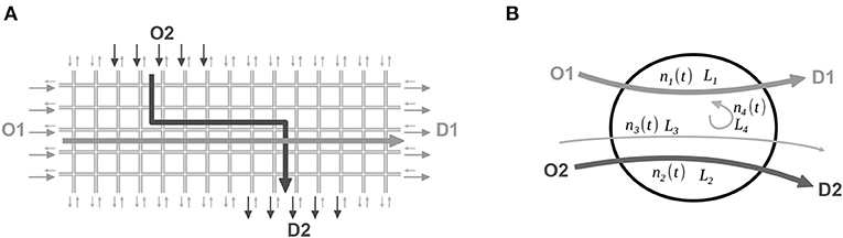
Figure 2. (A) Grid network with two major OD pairs and background traffic, and (B) single reservoir modeling with four routes.

3.2. Simulation Settings

Link-level traffic states are simulated by using the microsimulation platform Symuvia developed by LICIT (University of Lyon, France). This simulator is based on the car-following model of Newell (2002), the lane-changing model of Laval and Leclercq (2008) and further extensions for node merge models and multi-class traffic (Leclercq, 2007a,b; Chevallier and Leclercq, 2009; Leclercq and Laval, 2009). Network loading and unloading are investigated for a simulation duration of 20 h. Path flow distributions are updated for every period of 1 h 40 min to reach UE conditions. The convergence loop uses the classical Method of Successive Averages (MSA), involving the travel times of each path averaged over the last time period (Lu et al., 2009; Ameli et al., 2019). Two main flow directions are defined: O1-D1 aggregates all the trips from the West to the East boundary, and O2-D2 comprises all the trips from five entries in the North to five exits in the South boundary, as depicted in Figure 2A.

The demand scenarios for these trips always include a 30 min warm-up period, possibly followed by a high demand surge per origin O1 and/or O2. The total demand for a given macroscopic origin (O1 or O2) is equally distributed among its corresponding entry links. Each origin link flow is sent evenly to the exit links of the corresponding macroscopic destination (D1 for O1, D2 for O2). For a given macroscopic exit (D1 or D2), each exit link thus receives the same portion of the flow. Apart from the two main flows O1-D1 and O2-D2, the background traffic is set with a total constant demand of 0.075 veh/s evenly distributed among all the remaining entries and exits. A total constant demand of 0.035 veh/s is also set for the internal trips with the origin and destination links evenly distributed inside the network.

3.3. MFD-Based Modeling

In parallel to microsimulation, traffic states are predicted by a multi-trip single reservoir model, as described in section 2. The reservoir model includes four routes, i.e., 1, 2, 3, and 4, representing link-level trips from O1 to D1, from O2 to D2, and background and internal traffic, respectively (see Figure 2B). Based on our review in the previous section, different approaches will be studied, named as follows:

• MFD model 1/1: uses a pro-rata merge model at entry, and a decreasing diverge model at exit

• MFD model 1/2: uses a pro-rata merge model at entry, and a maximum diverge model at exit

• MFD model 2/2: uses an endogenous merge model at entry, and a maximum diverge model at exit

• MFD model 3/2: uses a FIFO merge model at entry, and a maximum diverge model at exit.

FIFO merge model is relevant when two different macropaths share the same entry gate into the reservoir. However, the entry gates for two major macropaths considered are independent and physically separated in the present work. Thus, FIFO merge model is only included to provide a complete overview of available entry flow functions proposed in the literature. The trip length of each route is estimated as the mean of all individual trips recorded in several microsimulations: L₁ = 1,850 m, L₂ = 1,250 m, L₃ = 1,350 m and L₄ = 1,330 m. These mean values may change by about 100 m from one simulation to another. The global routing in this network has been designed to obtain a significant difference between the trip lengths L₁ and L₂ of the two routes 1 and 2. The border capacities of O1 and O2 are calculated as: $C^1=C^2=5\times q_l$ = 3.6 veh/s.

The production-MFD P(n) of the grid network is estimated with several microsimulations of constant demand loading on all entries. Using a dynamic demand loading can introduce hysteresis phenomenon, thereby influencing the shape of the MFD. Hence, multiple microsimulations with each having a different constant demand is used to calibrate the production-MFD. The results of 8 different simulations are presented in Figure 3A, where total production and accumulation are aggregated over 10 min periods. This permits calibrating a piecewise linear MFD with maximum production P_c = 2,640 veh.m/s and two critical accumulations n_c1 = 660 veh, n_c2 = 1,700 veh defining the flat domain in P(n). The points that determine the congested branch of P(n) are obtained by limiting the network outflow exogenously. There are two ways of creating congestion in the network to estimate the congested branch of the MFD. The first is frequently used in other studies and consists in increasing the number of internal trips. Such scenarios favor the creation of local bottlenecks inside the network, thus reducing the average speed of all traveling vehicles. The second method instead focuses on the boundary conditions and exogenously limits the potential outflow of exit links. In this case, bottlenecks are explicitly generated at the network perimeter, from where congestion starts propagating until it finally reaches the entire network. In this study, we adopt this second method because we particularly focus on flow exchanges at the network borders. Thus, we want to calibrate an MFD that mainly describes the behavior of transferring trips. As for the exit demand function, the two models of P_d(n) are directly derived from P(n), as illustrated in Figure 3C.

FIGURE 3

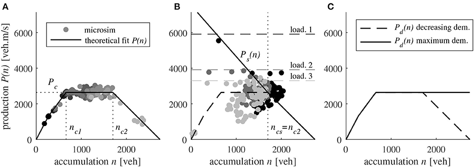
Figure 3. (A) Estimation of the production-MFD P(n) of the grid network using different constant demand loading scenarios in microsimulation, (B) the calibration of the entry production supply P_s(n) with three constant network loadings indicated by three different shades of gray, and (C) exit production demand P_d(n) for the two diverging approaches.

The first calibration of the entry supply function P_s(n) is shown in Figure 3B. In the first test, a simple way of calibrating P_s(n) consists in loading the network with a total entering production demand $\sum _{i=1}^4{L}_i{\lambda }_i$ higher than the MFD capacity P_c, with each macroscopic demand λ_i evenly distributed among all its corresponding entry links. As we know from the MFD calibration that the network cannot sustain a total production higher than P_c at equilibrium, we expect these loading simulations to provide an evolution of the total entering production as follows: from the warm-up level to the demand level $\sum _{i=1}^4{L}_i{\lambda }_i$, and from the demand level to P_c. This latter transient period should provide insight into how the inflows/entering productions adapt dynamically to the network capacity. Moreover, as we assumed that P_s(n) is an intrinsic property of the network, we need to run several loadings to ensure that a unique function is enough to describe the dynamic reduction of the total inflow. To this end, three constant loading scenarios were used to calibrate P_s(n), their respective evolutions in the (accumulation, production) plane are plotted in the same figure with three different shades of gray. While the total entering production demand $\sum _{i=1}^4{L}_i{\lambda }_i$ of each loading is greater than the MFD capacity P_c, we observe in the microsimulation that the traffic states always reach the critical accumulation n_c2 and stabilize around the capacity P_c. Thus, we conclude that n_cs = n_c2 is the critical accumulation of P_s(n) in this network configuration, delimiting saturated and over-saturated states in the reservoir. To be consistent with the MFD definition, for n > n_cs the entry supply function corresponds to the congested branch of P(n), because this branch was obtained precisely when the inflow equilibrated with the exogenous outflow limitation we set (see the description of the MFD estimation above). On the other hand, the estimation of P_s(n) for n ≤ n_cs was made using the highest demand loading case in Figure 3B. For this setting, in the microsimulation, the entering production decreases along the line of P_s(n) we plotted. This first calibration serves as a baseline for running the MFD simulations. Its relevance is investigated further in the following section on inflow merging.

4. Comparisons Between the Entry Merging Schemes With Network Loading Scenarios

The merging of inflows at the network entry is investigated with three sets of loading scenarios detailed below:

• Entry case 1: simulations with a high demand on route 1 and increased demand on route 2 at each simulation;

• Entry case 2: simulations with a high demand on route 2 and increased demand on route 1 at each simulation;

• Entry case 3: simulations with medium demands on routes 1 and 2, and increased demand on route 4 (internal traffic) at each simulation.

These test cases have been designed to stress the network by setting high demand flows at entry. At the same time, entry case with high demands on route 1 and 2 is avoided as it results in a very rapid gridlock with almost no insights into the flow dynamics. Thus, queues are observed spilling back to the entry links due to interactions between the two routes 1 and 2 in the middle of the network. Each simulation is run for 3 h, including a 30 min warm-up period followed by an instantaneous demand increase on both routes at the same time. The network traffic states reach steady states after ~1 h 30 min of simulation.

4.1. Investigation on the Network Entry Supply Function

Figure 4 shows the evolution of the total entering production $\sum _{i=1}^4{L}_i{q}_{\text{in},i}(t)$ in microsimulation for the three above-mentioned entry loading cases. For both cases 1 and 2, the demand of one route i is set to its border capacity Cⁱ = 3.6 veh/s (i = 1 for case 1 and i = 2 for case 2) while different simulations are run with an increased demand on the other route in each simulation. We note that the traffic states do not exactly reach the demand level during the loading. This is due to the aggregation period used to calculate the inflows in the microsimulation. This period must be higher than the signal cycle time of 1 min to smooth the inflow variations induced by green and red phases. While this period is generally of 5 min, shorter periods were chosen close to the demand surge to better observe the levels of entering production during the transient phase. But even with this adjustment, we see that the entering production almost reaches the demand level for <1 min, and then rapidly decreases. Then, the results are too scattered to identify a clear trend in the transition period of the network loading. This means that the intersections close to the entries are not operating at the maximum capacity of the entry links (including signal timings), but at a lower capacity due to interactions between turning vehicles. Here, it can be seen that this transition period depends on the demand settings in each simulation. This suggests that a single entry supply function P_s(n) cannot capture the variety of these transition periods. Whereas, it might constitute a reliable approximation for cases 1 and 3, we clearly see that the network loading of the simulations in case 2 is not well-described by the shape of P_s(n). Interestingly, the results in case 3 are less scattered and suggest a parabolic shape of P_s(n) for the transition period, which also depends on the loading level. Consequently, we see that in theory, a recalibration of the entry supply function would be required for each case if we want the MFD simulation to reproduce this transition period accurately. However, given the fact that in all cases, the shape we choose always leads to a reliable steady state near (n_c2, P_c), this shape can be considered acceptable if we want to preserve the generality of its application and not go into too much detail for the transient period. This modeling choice that we adopt for the rest of this study will also be discussed in the next subsection.

FIGURE 4

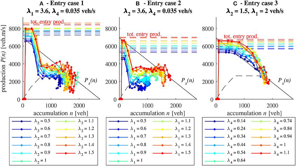
Figure 4. Evolution of total entering production $\sum _{i=1}^4{L}_i{q}_{\text{in},i}(t)$ in the (accumulation, production) plane for different network loading cases in microsimulation. The total entering production demand $\sum _{i=1}^4{L}_i{\lambda }_i$ is indicated by the dashed line. Each color corresponds to one simulation. (A) Results of entry case 1 for 11 simulations with increasing demand λ₂, (B) entry case 2 for 11 simulations with increasing demand λ₁, and (C) entry case 3 for 11 simulations with increasing demand λ₄.

4.2. Comparisons Between the Entry Merging Schemes

We now compare the two merging schemes presented in section 2.3 for a given network loading scenario from the entry case 2 (high demand on route 2). We investigate this case first as it gives the most obvious differences between the merging schemes. At equilibrium, we know, thanks to our previous investigations, that the total production is always around P_c. This will allow properly comparing the share of inflow or entering production between routes 1 and 2 in a steady state.

Figures 5A–C show the evolution of inflows, entering productions vs. time, and entering productions vs. total accumulation, respectively, in both the microsimulation and the MFD model 1/2. Figures 5D–F show the same results but for model 2/2; and Figures 5G–I also show the same results but for model 3/2. In this scenario of a sudden demand loading after 30 min, each inflow equals its corresponding demand, so that the first layer of our merge algorithm (applying the border limitations) is not involved here. But it is clear that both the reservoir inflow supply $P_s^{\text{ext}}(n)/L^{\text{ext}}$ for models 1/2 and 3/2, and production supply $P_s^{\text{ext}}(n)$ for model 2/2, limit the demand. In Figures 5C–I, clear discrepancies can be seen between the microsimulation and the MFD models during the transient period of the network loading. As noticed in the previous subsection, these discrepancies are due to the absence of recalibration of the entry supply function in this scenario. However, they only account for around 15 min of simulation (from t = 30 to 45 min), as shown in e.g., Figures 5D,E. As the steady-state of the total inflow q_in(t) and entering production $P_{\text{in}}(t)=\sum _{i=1}^4{L}_i{q}_{\text{in},i}(t)$ are well-reproduced by both MFD models, we conclude that the entry supply function we calibrate in Figure 3B is sufficient for our needs. We will show with more complex test cases in section 5 that the inflows from the microsimulation are well-estimated and that the discrepancies observed during the short transient phase of network loadings are negligible.

FIGURE 5

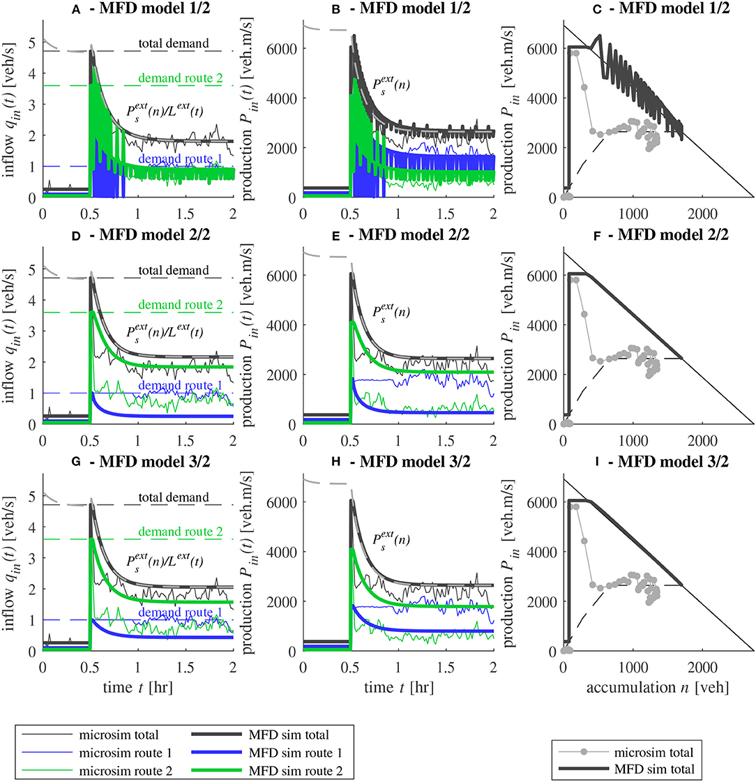
Figure 5. Comparison between microsimulation and two MFD models for a network loading case. (A) Evolution of inflows and (B) entering productions vs. time and (C) total entering production vs. total accumulation for model 1/2. (D) Evolution of inflows and (E) entering productions vs. time and (F) total entering production vs. total accumulation for model 2/2. (G) Evolution of inflows and (H) entering productions vs. time and (I) total entering production vs. total accumulation for model 3/2.

In Figures 5A,B, we observe numerical flow oscillations due to the demand pro-rata merge in model 1/2. This is due to the background traffic of route 3, which also undergoes a restricted inflow because of its small merge coefficient (proportional to demand). Thus, queuing vehicles are stored at entry, suddenly creating a maximum demand for route 3, which therefore has a higher merge coefficient. The result is that a higher flow portion is temporally allocated to route 3 to empty its small queue, and then to a smaller merge coefficient. This process is thus periodically repeated, entailing the oscillations. This is a well-known problem in merging models, with respect to the invariance principle (basically, here the model is not invariant as it oscillates when demand reaches capacity). It is the consequence of the demand pro-rata rule. This numerical phenomenon is mainly due to the point queue model used to account for the storage of vehicles at the entry of this single reservoir model, but the oscillations would likely disappear in a multi-reservoir context when vehicles are stored in another reservoir (also refer to the discussion in section 2.4).

However, despite this numerical issue, the demand pro-rata merge in model 1/2 is found to better reproduce the inflow or entering production share observed in microsimulation, in comparison to the endogenous merge in model 2/2 or the FIFO merge in model 3/2. This is quite obvious in steady-state, where the microsimulation results shows $q_{\text{in},1}^{*}\approx q_{\text{in},2}^{*}\approx$ 1 veh/s while model 2/2 predicts $q_{\text{in},1}^{*}\approx$ 0.1 veh/s and $q_{\text{in},2}^{*}\approx$ 1.9 veh/s (see Figures 5A,D). For model 2/2, the equilibrium inflow share is explained during the transient phase of the network loading. In this test, the maximum demand of route 2 is equal to 3.6 veh/s, which results in a higher increase of accumulation n₂(t) compared to n₁(t). Thus, in this model, since the endogenous coefficient assigned to route 2 is n₂(t)/(n₁(t) + n₂(t)), the greater the accumulation on this route, the more the flow can enter as this ratio becomes higher. This explains the significant difference between q_{in, 2}(t) and q_{in, 1}(t) after t = 30 min. Then, the system stabilizes to this share ratio because the same ratio of accumulations is implied in the outflow calculations, which naturally balances with the inflows. On the other hand, for model 1/2, the same trend is observed at the beginning of the loading just after t = 30 min, because the high demand on route 2 entails a higher allocation ratio for this route. However, as both routes become rapidly limited at entry, a queue forms for both of them and generates a high demand. Both routes are subject to the same demand because queuing vehicles want to enter as soon as possible regardless of their origin. By default, their maximum entrance rate is fixed to the border capacity Cⁱ = 3.6 veh/s as long as the queue for route i is not empty. With C¹ = C², the two merging coefficients are both equal to 0.5, which explains the identical steady inflows for both routes. As for model 3/2, we could expect similar results as model 1/2 because the FIFO merge of model 3/2 is also based on a demand pro-rata scheme. However, as explained in section 2.3, the FIFO merge model uses the demand share ratio at a time t₀ < t (when the vehicles enter the queue at entry) to allocate inflows at time t. Hence, routes 1 and 2 are not given the same allocation as route 2 has a higher demand than route 1, resulting in a higher inflow for route 2 as shown in Figure 5G. Note that this FIFO merge model implies that the vehicles are queuing together in a unique queue, which is actually not the case here (the entry borders of routes 1 and 2 are physically separated). This may thus explain the discrepancies between model 3/2 and the microsimulation results.

The three models 1/2, 2/2, and 3/2 are also compared against the microsimulation results for all the simulations of the three network loading cases. Figures 6A–C present the steady-state inflow for routes 1 and 2 obtained with the microsimulation and MFD models 1/2, 2/2, and 3/2, for entry cases 1, 2, and 3, respectively. In each simulation, the steady-state inflow is calculated as the mean inflow evolution from 1 h 30 min to 3 h. In each plot, one point corresponds to one simulation (one value of steady-state inflow per route). As illustrated in Figure 6B, the demand pro-rata merge in model 1/2 clearly better reproduces the inflow share observed in the microsimulation, in comparison to the endogenous merge in model 2/2 or the FIFO merge in model 3/2. This corroborates our first conclusion from Figure 5. Model 1/2 also provides a better estimation of the steady-state inflows in entry case 1, although bias can be noticed in the inflow in route 1 between the microsimulation outputs and all MFD models (see Figure 6A). In entry case 3, the difference between both MFD models is less obvious; nevertheless, model 1/2 appears more accurate than other models for predicting the outputs of the microsimulation, notably for the inflow in route 2 (see Figure 6C). In conclusion to this section, despite the bias that may appear in the calibration of P_s(n), the demand pro-rata merging scheme detailed in section 2.3 is shown to efficiently reproduce the inflow share observed in the microsimulation in a variety of situations. Note, however, that the comparison between the demand pro-rata and FIFO merge models is not quite fair, as a better comparison should be carried on another network configuration where the routes enter through the same boundary.

FIGURE 6

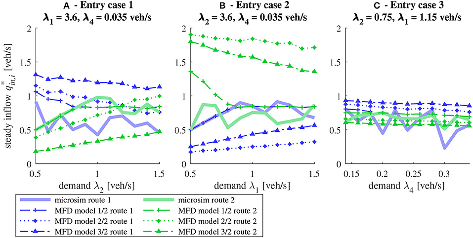
Figure 6. Comparison of steady state inflow per route between microsimulation and MFD models 1/2 and 2/2 for different network loading cases. (A) Results of entry case 1 for 11 simulations with increasing demand λ₂, (B) entry case 2 for 11 simulations with increasing demand λ₁, and (C) entry case 3 for 11 simulations with increasing demand λ₄.

5. Comparisons Between the Exit Diverging Schemes With Congestion Onset-Offset Scenarios

In this section, we present the comparisons between the microsimulation and MFD models 1/1 and 1/2 to investigate the effect of both exit diverge models: the decreasing outflow demand in over-saturation with the independent treatment of partial outflows (in model 1/1), and the maximum outflow demand in over-saturation with the inter-dependent treatment of partial outflows (in model 1/2), see section 2.2. In both MFD models, we use the demand pro-rata merge at entry, which was found to be the best option in the previous section. The demand scenarios for routes 1 and 2 consists of a 30 min warm-up period (around 0.1 veh/s) followed by a high demand surge of around 1 veh/s per origin O1 and/or O2 (equally distributed among entry links). Congestion is created inside the network by limiting the potential outflow from exit links in D1 and/or D2 below the corresponding origin demand. This supply limitation at the exits is then released at t₁ = 6 h 40 min. Finally, the high demand suddenly falls to its initial level after t₂ = 10 h to observe the full recovery of the network. Three test cases are investigated:

• Exit case 1: homogeneous outflow limitation is applied to the exits of D1 and D2

• Exit case 2: homogeneous outflow limitation is applied to the exits of D1 only

• Exit case 3: homogeneous outflow limitation is applied to the exits of D2 only.

The three exit cases are designed to generate different types of congestion spillbacks in the network. Owing to the differences in the trip lengths of macropaths, spillbacks originating from D2 will have a different effect on the network than the ones from D1. Their demand and supply scenarios are presented in Figures 7A–C, respectively. Note that these simulation settings are not intended to correspond to any real situations, the high demands and their long durations are designed to stress the network and to observe clear congestion wave propagation until the next steady-state. In the microsimulation, accumulation, inflow and outflow are calculated for every 5 min aggregation period. After running the MFD simulations, we filter the inflow oscillations generated by the pro-rata merge coefficients. This helps when presenting the results because only the mean value is of importance for our analysis.

FIGURE 7

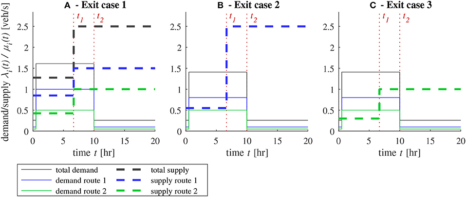
Figure 7. (A) Demand and supply scenario of exit case 1, (B) exit case 2, and (C) exit case 3.

5.1. Exit Case 1: Outflow Limitation on Both Routes

The results for the first case are given in Figure 8. The corresponding demand and supply settings are presented in Figure 7A. The evolutions of accumulations, inflows and outflows in microsimulation are compared against the predictions of each MFD model: in Figures 8A–C for model 1/1, and Figures 8D–F for model 1/2. Several interesting observations can be made, as detailed below.

FIGURE 8

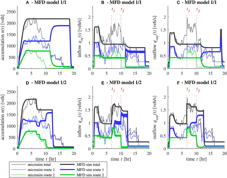
Figure 8. Comparison between microsimulation and different MFD models for case 1: exit limitation on both routes. Times t₁ and t₂ corresponding to supply release and demand decrease, respectively, are indicated. (A) Evolution of accumulation, (B) inflow, and (C) outflow with model 1/1, (D) accumulation, (E) inflow, and (F) outflow with model 1/2.

We first focus on the period [0, t₁], which corresponds to the onset of congestion due to the high increase in demand above the outflow limitations for both routes. At the network exit, all the results show that the outflow of route 2 remains equal to its limitation while the outflow of route 1 decreases after t = 2 h. This is due to the interaction between the two routes in the middle of the network: the vehicles traveling longer trips on route 1 are blocked by congestion on route 2, which spills back faster because of shorter distances. This is quite well-reproduced in both MFD models.

We then focus on the second period, from time t₂ to the end of the simulation, when all outflow limitations are released. As hypothesized and highlighted in MFD simulation by Mariotte et al. (2017) and Mariotte and Leclercq (2019), it clearly appears that the decreasing exit demand function in model 1/1 prevents the reservoir from recovering after the congestion period. In Figure 8C, it can be seen that the outflows do not react to the release of exit limitations after t₁, whereas the microsimulation exhibits a sudden increase of outflow at this time. On the contrary, model 1/2 using the maximum exit demand function adequately reproduces the queue discharge at the network exit after t₁. Then, the network can finally recover after t₂ once the demands fall to their initial levels. Model 1/1 is still able to recover because of the fall in demand at entry after t₂, but the assumption of a low outflow demand results in a much longer congestion period. Congestion vanishes just before t = 20 h, which is nearly twice as long as in model 1/2. However, this model overestimates the outflow of route 1 after t₂, as it predicts a high and fast discharge of the remaining vehicles in the reservoir. This is not the case in the microsimulation, where residual congestion is observed in route 1 until t = 17 h. The outflow of route 1 is lower and thus, the time needed to empty the queues on this route is longer in comparison to the MFD simulation. This phenomenon is the result of internal congestion that can be captured by link-level simulation, but this is hardly reproducible in MFD models. One possible solution would be to adjust the exit demand function P_d(n), for which two opposite approaches have been presented in Equations (4) and (5). Based on this comparative analysis, it appears that the decreasing exit demand model is too pessimistic to reproduce internal congestion. On the other hand, the maximum exit demand model works nicely for short routes like route 2 in this case, but it is too optimistic for longer routes where residual queues need more time to empty. The differences between both routes exhibited in microsimulation are the results of the heterogeneity of traffic states inside the network. Thus, an exit demand function that would work in any situation is impossible to design if such a function is based on a unique MFD P(n), because of the mean speed assumption shared by all vehicles.

The conclusion of this test case comparison is that the best match with microsimulation outputs is obtained with model 1/2, with the maximum exit demand function.

5.2. Exit Case 2: Outflow Limitation on Route 1 Only

The results for the second case are given in Figure 9. The corresponding demand and supply settings are presented in Figure 7B. The evolutions of accumulations, inflows and outflows in microsimulation are compared against the predictions of each MFD model: in Figures 9A–C for model 1/1, and Figures 9D–F for model 1/2.

FIGURE 9

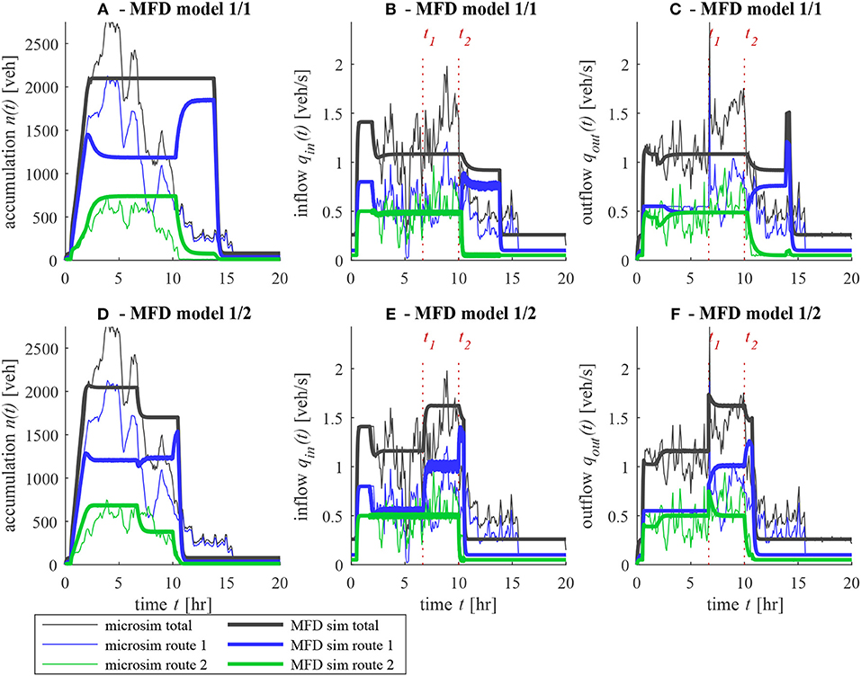
Figure 9. Comparison between microsimulation and different MFD models for case 2: exit limitation on route 1. Times t₁ and t₂ corresponding to supply release and demand decrease, respectively, are indicated. (A) Evolution of accumulation, (B) inflow, and (C) outflow with model 1/1, (D) accumulation, (E) inflow, and (F) outflow with model 1/2.

In this scenario, similar observations can be made as compared to exit case 1. From t = 0 to t₁, both models 1/1 and 1/2 provide, on average, a reliable estimation of the inflows and outflows of the microsimulation. However, considerable scatter in these flow values given by the microsimulation. This scatter results in significant variations observed in the evolution of accumulations, in particular for route 1, as shown in Figures 9A,D. As in exit case 1 after t₁, model 1/1 fails to reproduce the queue release as the outflow of route 1 remains low and equal to its previous exogenous limitation of μ₁ = 0.5 veh/s, applied during [0, t₁]. On the other hand, the queue discharge observed in the microsimulation is quite well-predicted by model 1/2 after t₁. Because of the scatter in the microsimulation outputs, in this case, the increase of outflow of both routes after t₁ is less obvious than in exit case 1. As with the latter case, residual congestion can be seen in Figures 9C,F in the microsimulation results. Again, none of the MFD models is able to describe it; however, model 1/2 is still the most accurate regarding the whole simulation period. The evolution of traffic states on route 2 is particularly well-reproduced with model 1/2, as presented in Figures 9D–F. The conclusions in this test case are hence the same as in exit case 1.

5.3. Exit Case 3: Outflow Limitation on Route 2 Only

The results for the third case are given in Figure 10. The corresponding demand and supply settings are presented in Figure 7C. The evolutions of accumulations, inflows and outflows in microsimulation are compared against the predictions of each MFD model: in Figures 10A–C for model 1/1, and Figures 10D–F for model 1/2.

FIGURE 10

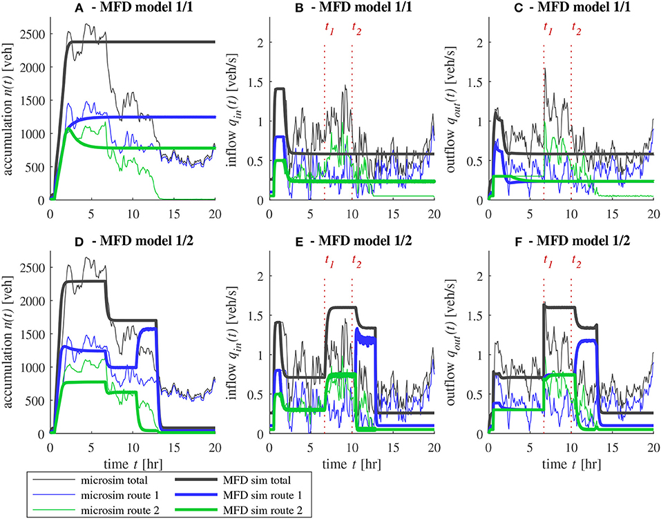
Figure 10. Comparison between microsimulation and different MFD models for case 3: exit limitation on route 2. Times t₁ and t₂ corresponding to supply release and demand decrease, respectively, are indicated. (A) Evolution of accumulation, (B) inflow, and (C) outflow with model 1/1, (D) accumulation, (E) inflow, and (F) outflow with model 1/2.

First, during the onset of congestion before t₁, we can clearly see in Figures 10C,F the outflow limitation of route 2 and its impact on the outflow of route 1. The latter is significantly reduced, although no exogenous limitation is applied on this route in this test case. Likewise, with exit case 1, it is interesting to note that during the first 2 h of the simulation, model 1/1 adequately reproduces the high outflow of route 1, while model 1/2 clearly misses this outflow peak. This underestimation is even more significant in this case than in case 1, due to the diverge outflow model. When using the maximum exit demand assumption, Mariotte and Leclercq (2019) showed that explicit inter-dependency relationships must be employed, as presented in equation 8. While ensuring consistent, steady states after congestion onset, as we can see after t = 2 h, the drawback is that these relationships are applied instantaneously to route outflows. Consequently, once the outflow of route 2 is limited at the very beginning of the simulation, that of route 1 is instantaneously reduced to accommodate this limitation through the formula in Equation (8). In this case, the exit of route 2 is that which is most constrained, as described in Equation (7). The situation is different with the other diverge outflow model in model 1/1. Because each exit limitation is applied independently, the outflow of route 1 can reach the flow level sent by the entry earlier, as can be seen in Figure 10C. But after t = 2 h, the increase of accumulation in the reservoir due to the onset of congestion causes the mean speed to decrease, and thus reduces the potential outflow of route 1 to finally reach almost the same steady-state as in model 1/2. In this approach, the interaction between the route outflows is implicitly described through the speed or production-MFD. Regarding the microsimulation results, it appears that this approach is, therefore, better for transient evolution during congestion onset.

However, during the offset of congestion after t₁, the diverge outflow of model 1/1 is unable to predict the queue discharge on route 2 once its corresponding limitation is released at the exit (see Figure 10C). This is similar to what we observed in exit cases 1 and 2. Here also, model 1/2 provides better results for congestion offset, although the total outflow is noticeably overestimated after t₂. This model anticipates the unloading of route 1 at the same time as for route 2, due to the inter-dependency relationships mentioned above. But this does not occur in the microsimulation as this outflow remains low. The simulation duration is not long enough to observe full network recovery, and residual congestion on route 1 is still observed at t = 20 h. Hence, the exit demand of model 1/2 is again too optimistic for the congestion offset, while the exit demand of model 1/1 is clearly too pessimistic. Though not presented here, model 1/1 is still able to recover due to the decrease in demand at entry after t₂. But the assumption of a low outflow demand results in a much longer congestion period. If we run the MFD simulation for a longer time frame, the offset of congestion appears at t = 24 h, nearly twice as long as in model 1/2.

In conclusion, for this test case, although no MFD approach was found to be fully satisfactory to reproduce the microsimulation results due to local congestion (high link-level heterogeneity), the maximum exit demand function of model 1/2 can at least match the evolution of traffic states in route 2 quite well.

6. Conclusion

In this paper, we compared different MFD models against microsimulation on an artificial grid network crossed by two regional flows having different mean trip distances. The MFD frameworks we tested include three inflow merge models (demand pro-rata merge with flow merge from the literature, our endogenous merge with production merge, and a new FIFO flow merge), and two outflow diverge models (decreasing outflow demand in oversaturation with the independent treatment of partial outflows from the literature, and our maximum outflow demand in oversaturation with the interdependent treatment of partial outflows). The first contribution of this paper was to propose a unified two-layer merging scheme with an entry supply function to handle the inflow merge models. Thanks to microsimulation, the reservoir entry supply function was calibrated with several network loading scenarios. A thorough analysis of these loading cases with different demand patterns showed that the shape of this function might not be unique, as it depends on the demand configuration for its undersaturated branch. However, this non-uniqueness would be critical only during the transient period of the network loading, because our results also showed that an identical equilibrium point is almost always reached in the production-MFD. As the transition period was found to be quite short in our loading simulation tests, the calibration issue of the entry supply function in undersaturation would not be a major source of error in a general case.

The second contribution was the comparison of the different merge models and diverge models. At the network entry, three sets of 11 simulations were used to study various situations of network loading cases. In all these situations, we found that the demand pro-rata merging model provided a better estimation of flow equilibrium after the congestion onset, in comparison to the endogenous and FIFO merge models. Nevertheless, our comparison relies on the perfect independence of the queuing vehicles at entry, which is not universally expected. As we mentioned, this may temper our conclusion on merge models, especially when there are inter-dependent vehicle queues, because stored in the same reservoir in a multi-reservoir framework. Further investigations are therefore still needed on merge models when several reservoirs are connected together.

At the network exit, three test cases of a long scenario with congestion onset and offset were thoroughly investigated. The following observations were made. While adequately reproducing transient states during congestion onset, the approach of a decreasing outflow demand was found to be too pessimistic to predict the unloading of queues once the exit limitations were released. On the other hand, the approach assuming a maximum outflow demand led to better results. Nevertheless, the drawback of the latter framework was that inter-dependency between all the partial outflows had to be explicitly formulated in the diverging outflow scheme to comply with the reservoir mean speed hypothesis (homogeneity in traffic states). This resulted in faster network recovery in comparison to the microsimulation outputs, where local link-level interactions generated more internal congestion than predicted by the MFD simulation. Interestingly, more internal congestion was found in the case when spillbacks on shorter routes interacted with under-saturated traffic flows on longer routes. Such a scenario is likely to generate more heterogeneous traffic states and be thus more challenging for MFD-based simulation. Nevertheless, while being rather optimistic during congestion offset, on the whole, the approach of the maximum outflow demand proved capable of overcoming the issues encountered with the approach of decreasing outflow demand generally adopted in the literature. The latter results still need to be confirmed with other network and demand configurations. It is also worth noting that multi-reservoir models (Mariotte and Leclercq, 2019) use a hybrid approach as internal trips (trips that end inside the reservoir) follow the decreasing diverge outflow model and transfer trips (trips that leave the reservoir) follows the maximum diverge model. Inflows and outflows for internal trips should have special treatments as they can start or end anywhere within the reservoir and should not be restricted by perimeter constraints. As such, it is assumed that internal inflow is unrestricted and that internal outflow (the rate at which the users reach their destination) decreases proportionally to the production-MFD.

Our simulation case was designed to create strong internal correlations between the two major flows, which is certainly a limit case compared to reality. However, it provided a better overview of the aggregation of microscopic dynamics and the way MFD models reproduce it. Thus, further work on more complex simulation cases and real field studies are essential to corroborate these results, especially with more OD options on bigger networks. Internal congestion can be a consequence of several microscopic phenomena, such as traffic signals, routing choice, driver behavior, vehicle characteristics etc. By including such phenomena can have a significant influence on the microsimulation results and shape of the underlying MFD (Buisson and Ladier, 2009; Keyvan-Ekbatani et al., 2019). At the same time, it is impossible to separate each individual phenomenon's effect on the evolution of flow dynamics at the entry and exit. The proposed test case aims to quantify the interactions of the vehicles that are traveling between different OD pairs and their influence on the inflow and outflow dynamics. Hence, a more simplistic case is considered here by minimizing the unwanted phenomena on the traffic dynamics. The inflows and outflows observed in the current case are solely due to the interactions of vehicles at the intersections, which creates congestion bottlenecks, and eventually, spillbacks. For the same reason, a constant traffic signal time settings with zero offset is chosen in the present work. Nonetheless, it would be an interesting contribution to analyze the flow dynamics with more realistic test cases to verify the validity of the present conclusions. The present work lays the foundation for future works by providing some critical conclusions on managing the flows at entry and exits in MFD-based models. It gives a clear idea of how flow dynamics evolve at the extremities in the absence of complex situations and provides a fundamental base that can be included in the MFD-based framework. Using this knowledge and further tests on real networks, it is possible to embed more phenomena into these functions to capture the flow dynamics more accurately and realistically.

Data Availability Statement

The raw data supporting the conclusions of this article will be made available by the authors, without undue reservation.

Author Contributions

GM and LL: study conception and design. MP: microsimulation settings. GM: MFD simulation settings and draft manuscript preparation. GM, LL, and MP: analysis and interpretation of results. LL: supervision. All authors reviewed the results and approved the final version of the manuscript.

Funding

This project received funding from the European Research Council (ERC) under the European Union's Horizon 2020 research and innovation program (grant agreement No 646592—MAGnUM project).

Conflict of Interest

The authors declare that the research was conducted in the absence of any commercial or financial relationships that could be construed as a potential conflict of interest.

Acknowledgments

The content of this article has been published in Chapter 5 as part of the thesis of Guilhem Mariotte (see Mariotte, 2018).

References

Aboudolas, K., and Geroliminis, N. (2013). Perimeter and boundary flow control in multi-reservoir heterogeneous networks. Transport. Res. B Methodol. 55, 265–281. doi: 10.1016/j.trb.2013.07.003

CrossRef Full Text | Google Scholar

Ameli, M., Lebacque, J.-P., and Leclercq, L. (2019). “Multi-attribute, multi-class, trip-based, multi-modal traffic network equilibrium model: application to large-scale network,” in Traffic and Granular Flow 17 (Washington, DC: Springer), 487–495. doi: 10.1007/978-3-030-11440-4_53

CrossRef Full Text | Google Scholar

Batista, S., Ingole, D., Leclercq, L., and Menendez, M. (2020). The role of trip lengths calibration in model-based perimeter control strategies. IEEE Trans. ITS.

Batista, S. F. A., Leclercq, L., and Geroliminis, N. (2019). Estimation of regional trip length distributions for the calibration of the aggregated network traffic models. Transport. Res. B Methodol. 122, 192–217. doi: 10.1016/j.trb.2019.02.009

CrossRef Full Text | Google Scholar

Buisson, C., and Ladier, C. (2009). Exploring the impact of homogeneity of traffic measurements on the existence of macroscopic fundamental diagrams. Transport. Res. Rec. 2124, 127–136. doi: 10.3141/2124-12

CrossRef Full Text | Google Scholar

Chevallier, E., and Leclercq, L. (2009). Do microscopic merging models reproduce the observed priority sharing ratio in congestion? Transport. Res. C Emerg. Technol. 17, 328–336. doi: 10.1016/j.trc.2009.01.002

CrossRef Full Text | Google Scholar

Daganzo, C. F. (1994). The cell transmission model: a dynamic representation of highway traffic consistent with the hydrodynamic theory. Transport. Res. B Methodol. 28, 269–287. doi: 10.1016/0191-2615(94)90002-7

CrossRef Full Text | Google Scholar

Daganzo, C. F. (1995). The cell transmission model, part II: network traffic. Transport. Res. B Methodol. 29, 79–93. doi: 10.1016/0191-2615(94)00022-R

CrossRef Full Text | Google Scholar

Daganzo, C. F. (2007). Urban gridlock: macroscopic modeling and mitigation approaches. Transport. Res. B Methodol. 41, 49–62. doi: 10.1016/j.trb.2006.03.001

CrossRef Full Text | Google Scholar

Ge, Q., and Fukuda, D. (2019). A macroscopic dynamic network loading model for multiple-reservoir system. Transport. Res. B Methodol. 126, 502–527. doi: 10.1016/j.trb.2018.06.008

CrossRef Full Text | Google Scholar

Geroliminis, N. (2009). “Dynamics of peak hour and effect of parking for congested cities,” in Transportation Research Board 88th Annual Meeting, 09-1685 (Washington DC).

Google Scholar

Geroliminis, N. (2015). Cruising-for-parking in congested cities with an mfd representation. Econ. Transport. 4, 156–165. doi: 10.1016/j.ecotra.2015.04.001

CrossRef Full Text | Google Scholar

Geroliminis, N., and Daganzo, C. F. (2007). “Macroscopic modeling of traffic in cities,” in Transportation Research Board 86th Annual Meeting, 07-0413 (Washington DC).

Google Scholar

Haddad, J. (2015). Robust constrained control of uncertain macroscopic fundamental diagram networks. Transport. Res. C Emerg. Technol. 59, 323–339. doi: 10.1016/j.trc.2015.05.014

CrossRef Full Text | Google Scholar

Haddad, J. (2017). Optimal perimeter control synthesis for two urban regions with aggregate boundary queue dynamics. Transport. Res. B Methodol. 96, 1–25. doi: 10.1016/j.trb.2016.10.016

CrossRef Full Text | Google Scholar

Haddad, J., and Mirkin, B. (2020). Resilient perimeter control of macroscopic fundamental diagram networks under cyberattacks. Transport. Res. B Methodol. 132, 44–59. doi: 10.1016/j.trb.2019.01.020

CrossRef Full Text | Google Scholar

Hajiahmadi, M., Knoop, V., De Schutter, B., and Hellendoorn, H. (2013). “Optimal dynamic route guidance: a model predictive approach using the macroscopic fundamental diagram,” in 2013 16th International IEEE Conference on Intelligent Transportation Systems (ITSC) (The Hague), 1022–1028. doi: 10.1109/ITSC.2013.6728366

CrossRef Full Text | Google Scholar

Jin, W., and Zhang, H. (2004). Multicommodity kinematic wave simulation model for network traffic flow. Transport. Res. Rec. 1883, 59–67. doi: 10.3141/1883-07

CrossRef Full Text | Google Scholar

Keyvan-Ekbatani, M., Gao, X. S., Gayah, V. V., and Knoop, V. L. (2019). Traffic-responsive signals combined with perimeter control: investigating the benefits. Transport. B Transport Dyn. 7, 1402–1425. doi: 10.1080/21680566.2019.1630688

CrossRef Full Text | Google Scholar

Keyvan-Ekbatani, M., Kouvelas, A., Papamichail, I., and Papageorgiou, M. (2012). Exploiting the fundamental diagram of urban networks for feedback-based gating. Transport. Res. B Methodol. 46, 1393–1403. doi: 10.1016/j.trb.2012.06.008

CrossRef Full Text | Google Scholar

Keyvan-Ekbatani, M., Papageorgiou, M., and Knoop, V. L. (2015). Controller design for gating traffic control in presence of time-delay in urban road networks. Transport. Res. C Emerg. Technol. 59, 308–322. doi: 10.1016/j.trc.2015.04.031

CrossRef Full Text | Google Scholar

Kim, S., Tak, S., and Yeo, H. (2018). Investigating transfer flow between urban networks based on a macroscopic fundamental diagram. Transport. Res. Rec. 2672, 75–85. doi: 10.1177/0361198118778927

CrossRef Full Text | Google Scholar

Knoop, V. L., and Hoogendoorn, S. P. (2014). “Network transmission model: a dynamic traffic model at network level,” in Transportation Research Board 93rd Annual Meeting, 14-1104 (Washington DC).

Google Scholar

Kouvelas, A., Saeedmanesh, M., and Geroliminis, N. (2017). Enhancing model-based feedback perimeter control with data-driven online adaptive optimization. Transport. Res. B Methodol. 96, 26–45. doi: 10.1016/j.trb.2016.10.011

CrossRef Full Text | Google Scholar

Laval, J. A., and Leclercq, L. (2008). Microscopic modeling of the relaxation phenomenon using a macroscopic lane-changing model. Transport. Res. B Methodol. 42, 511–522. doi: 10.1016/j.trb.2007.10.004

CrossRef Full Text | Google Scholar

Leclercq, L. (2007a). Bounded acceleration close to fixed and moving bottlenecks. Transport. Res. B Methodol. 41, 309–319. doi: 10.1016/j.trb.2006.05.001

CrossRef Full Text | Google Scholar

Leclercq, L. (2007b). Hybrid approaches to the solutions of the “Lighthill-Whitham-Richards” model. Transport. Res. B Methodol. 41, 701–709. doi: 10.1016/j.trb.2006.11.004

CrossRef Full Text | Google Scholar

Leclercq, L., and Becarie, C. (2012). “Meso Lighthill-Whitham and Richards model designed for network applications,” in Transportation Research Board 91st Annual Meeting, 12-0387 (Washington DC).

Google Scholar

Leclercq, L., and Laval, J. A. (2009). “A multiclass car-following rule based on the LWR model,” in Traffic and Granular Flow '07 (Berlin; Heidelberg: Springer Berlin Heidelberg), 151–160. doi: 10.1007/978-3-540-77074-9_13

CrossRef Full Text | Google Scholar

Lentzakis, A. F., Ware, S. I., and Su, R. (2016). “Region-based dynamic forecast routing for autonomous vehicles,” in 2016 IEEE 19th International Conference on Intelligent Transportation Systems (ITSC), 1464–1469. doi: 10.1109/ITSC.2016.7795750

CrossRef Full Text | Google Scholar

Lu, C.-C., Mahmassani, H. S., and Zhou, X. (2009). Equivalent gap function-based reformulation and solution algorithm for the dynamic user equilibrium problem. Transport. Res. B Methodol. 43, 345–364. doi: 10.1016/j.trb.2008.07.005

CrossRef Full Text | Google Scholar

Mariotte, G. (2018). Dynamic modeling of large-scale urban transportation systems (Ph.D. thesis), University of Lyon, Lyon, France.

Google Scholar

Mariotte, G., and Leclercq, L. (2019). Flow exchanges in multi-reservoir systems with spillbacks. Transport. Res. B Methodol. 122, 327–349. doi: 10.1016/j.trb.2019.02.014

CrossRef Full Text | Google Scholar

Mariotte, G., Leclercq, L., Batista, S. F. A., Krug, J., and Paipuri, M. (2020). Calibration and validation of multi-reservoir MFD models: a case study in Lyon. Transport. Res. B Methodol. 136, 62–86. doi: 10.1016/j.trb.2020.03.006

CrossRef Full Text | Google Scholar

Mariotte, G., Leclercq, L., and Laval, J. A. (2017). Macroscopic urban dynamics: analytical and numerical comparisons of existing models. Transport. Res. B Methodol. 101, 245–267. doi: 10.1016/j.trb.2017.04.002

CrossRef Full Text | Google Scholar

Newell, G. F. (2002). A simplified car-following theory: a lower order model. Transport. Res. B Methodol. 36, 195–205. doi: 10.1016/S0191-2615(00)00044-8

CrossRef Full Text | Google Scholar

Paipuri, M., and Leclercq, L. (2020). Bi-modal macroscopic traffic dynamics in a single region. Transport. Res. B Methodol. 133, 257–290. doi: 10.1016/j.trb.2020.01.007

CrossRef Full Text | Google Scholar

Paipuri, M., Xu, Y., Gonzalez, M. C., and Leclercq, L. (2020). Estimating mfds, trip lengths and path flow distributions in a multi-region setting using mobile phone data. Transport. Res. C Emerg. Technol. 118:102709. doi: 10.1016/j.trc.2020.102709

CrossRef Full Text | Google Scholar

Ramezani, M., Haddad, J., and Geroliminis, N. (2015). Dynamics of heterogeneity in urban networks: aggregated traffic modeling and hierarchical control. Transport. Res. B Methodol. 74, 1–19. doi: 10.1016/j.trb.2014.12.010

CrossRef Full Text | Google Scholar

Sirmatel, I. I., and Geroliminis, N. (2017). Economic model predictive control of large-scale urban road networks via perimeter control and regional route guidance. IEEE Trans. Intell. Transport. Syst. 19, 1112–1121. doi: 10.1109/TITS.2017.2716541

CrossRef Full Text | Google Scholar

Sirmatel, I. I., and Geroliminis, N. (2019). Nonlinear moving horiz estimation for large-scale urban road networks. IEEE Trans. Intell. Transport. Syst. 1–12. doi: 10.1109/TITS.2019.2946324

CrossRef Full Text

Wada, K., Satsukawa, K., Smith, M., and Akamatsu, T. (2019). Network throughput under dynamic user equilibrium: queue spillback, paradox and traffic control. Transport. Res. B Methodol. 126, 391–413. doi: 10.1016/j.trb.2018.04.002

CrossRef Full Text | Google Scholar

Yildirimoglu, M., and Geroliminis, N. (2014). Approximating dynamic equilibrium conditions with macroscopic fundamental diagrams. Transport. Res. B Methodol. 70, 186–200. doi: 10.1016/j.trb.2014.09.002

CrossRef Full Text | Google Scholar

Yildirimoglu, M., Ramezani, M., and Geroliminis, N. (2015). Equilibrium analysis and route guidance in large-scale networks with mfd dynamics. Transport. Res. C Emerg. Technol. 59, 404–420. doi: 10.1016/j.trc.2015.05.009

CrossRef Full Text | Google Scholar

Zhang, Z., Wolshon, B., and Dixit, V. V. (2015). “Integration of a cell transmission model and macroscopic fundamental diagram: network aggregation for dynamic traffic models,” in Transport. Res. C Emerg. Technol. 55, 298–309. doi: 10.1016/j.trc.2015.03.040

CrossRef Full Text | Google Scholar

Zhong, R., Huang, Y., Chen, C., Lam, W., Xu, D., and Sumalee, A. (2018). Boundary conditions and behavior of the macroscopic fundamental diagram based network traffic dynamics: a control systems perspective. Transport. Res. B Methodol. 111, 327–355. doi: 10.1016/j.trb.2018.02.016

CrossRef Full Text | Google Scholar