Modelling autonomous vehicle interactions with bicycles in traffic simulation

1 Introduction

Testing of autonomous vehicle functions in real-world scenarios with Vulnerable Road Users (VRUs) such as bicyclists is a key stage on the way to developing fully functioning autonomous vehicles. Recently, evaluating vehicle models in simulation and virtual environments has become a very important intermediate step that reduces costs and avoids potential safety critical situations during the development phase. Virtual tests now include all the different components of a self-driving car. The different manufacturers partly rely on their own in-house simulations, but there are already many open-source programs on the market, some of which even support autonomous vehicle models, such as CARLA, developed by (Dosovitskiy et al., 2017). Microscopic traffic simulation tools such as Simulation of Urban Mobility (SUMO) (Lopez et al., 2018), VISSIM (PTV AG, 2016), and AIMSUN (Barceló and Casas, 2005), which are originally developed for the simulation of vehicle flows in microscopic traffic scenarios, still lack an interface to perform simulations with mixed traffic volumes composed of VRUs and autonomous vehicles. This paper proposes an autonomous vehicle model for use in microscopic traffic simulation focusing on modeling interactions with bicycle traffic. The proposed autonomous vehicle architecture is based on the four most important components of a self-driving car: Perception, Planning, Control, and Communication. Most importantly, the model integrates sensor models for the perception component that identify nearby simulated users and makes use of path-finding algorithms used predominately in the field of robotics and autonomous vehicle research for accomplishing driving tasks and interacting with bicycle traffic.

This paper is divided into three parts. At the beginning, the state of the art of the individual autonomous vehicle components is analyzed with regard to different functions of the model developed. In addition, various research approaches, such as the used path-finding algorithms, are examined. The developed autonomous vehicle model is based on the different components of a self-driving car: Perception, Planning, Control, and Communication. In order to test the implemented control logic and the interface with SUMO, four test scenarios where the autonomous vehicle model has to perform common driving tasks and interact with simulated bicyclists are developed, and the behavior of the vehicle model is examined. The behavior of the simulated bicycle agent in these scenarios is derived from the behavior of real test subjects that took part in bicycle simulator studies conducted at the Chair of Traffic Engineering and Control at the Technical University of Munich (TUM). Finally the performance and behavior of the autonomous vehicle model is compared to the existing car-following models (CFMs) and the lane changing models, which are already part of the SUMO simulation software. The driving behavior of the individual models is then assessed with key traffic safety and performance parameters. The proposed methodology is developed in the context of the @City Project, which aims to develop new automated driving functions for urban traffic scenarios.

2 Methods

2.1 Simulation environments

Since newly developed automated vehicle functions can only be tested in combination with respective testing scenarios, various companies and open-source projects have already developed promising platforms for evaluations. For example, with the NVIDIA Drive Constellation, NVIDIA provides an open platform based on a virtual test fleet for the validation of autonomous vehicles NVIDIA (2019). To evaluate the individual models, the solution relies on the key elements of simulation and the possibility of a subsequent replay allowing for data evaluation and analysis. CARLA is a software simulator for autonomous driving supporting development, training, and validation of autonomous urban driving systems. It supports different sensor specifications and environmental conditions combined with three self-driving approaches: a classic modular pipeline, an end-to-end model trained via imitation learning, and an end-to-end model trained via reinforcement learning (Dosovitskiy et al., 2017). It also offers an integration with SUMO and VISSIM for simulating traffic flow. These environments can be eventually integrated with physical simulators that enable interconnected studies with real test subjects assuming the role of a driver, pedestrian, or bicyclist. In order to study the behavior of bicyclists in traffic, a bicycle simulator is introduced Keler et al. (2018). The bicycle simulator has the purpose of collecting trajectories of test subjects experiencing traffic scenarios, interacting with other simulated road users, and transport infrastructure. The bicycle simulator consists of a physical bicycle fitted with speed and steering sensors connected to a micro-controller, which sends the measurements to a model (MATLAB Simulink) within the driving simulation software DYNA4 from the company TESIS, part of Vector Informatic GmbH. Microscopic traffic simulation is handled by SUMO via a bridge module between SUMO and DYNA4. The bicycle simulator setup is presented in Figure 1 For increasing simulation accuracy and quality, the development of high quality models is of utmost importance. In microscopic traffic simulation software such as SUMO, VISSIM, and AIMSUN Barceló and Casas (2005) that can be coupled with simulators used for autonomous vehicle research such as CARLA or DYNA4, motor traffic is modeled through the implementation of car-following models that adapt the agent’s behavior based on the position and speed of the leading vehicle. The lateral movement is usually adapted through a discrete lane choice model and in the case of mixed traffic simulation through the resolution of a traffic lane into sub-lanes or through non-lane-based behavior using the maximum longitudinal time to collision (TTC) to choose the lateral position along a lane Lopez et al. (2018); PTV AG (2016); Fellendorf and Vortisch (2010); Semrau and Erdmann (2016). Therefore, the integration of autonomous driving functions in the existing models becomes a difficult and time-consuming procedure, as it requires the adaptation of existing model functions. Additionally, the motion of the simulated agents remains confined by the resolution of the traffic space into lanes and other simulator-specific network elements, which in turn limits the simulation accuracy for advanced autonomous driving functions, especially in cases with interactions with other simulated agents.

FIGURE 1

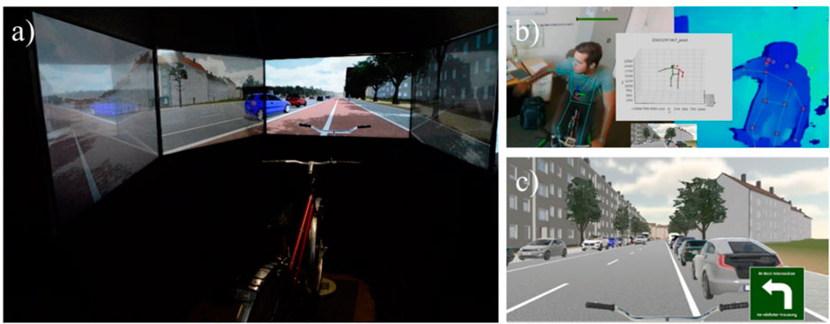
FIGURE 1. (A) Bicycle simulator setup, (B) skeletal points extraction and depth field detection, (C) 3D simulator environment.

2.2 Basic autonomous agent model

In order to address the existing limitations identified in the literature review executed in the process of this project, an approach for modeling and studying autonomous vehicle and bicycle interactions is proposed. The proposed autonomous agent model relies on the four elements used in the development of autonomous vehicles Perception, Planning, Control, and Communication. In order to combine these controlling devices, the agent is fitted with a main Controlling Unit, which is responsible for connecting the various parts of the control in a main control system taking care of when to use specific sub-controllers. The main control loop is shown in Figure 2 given by Algorithm 1. Its architecture is based on the general autonomous vehicle control components described in the literature review and the layout proposed in Kogan and Murray (2006), extending it to work for implementation in a simulation software environment. The model is implemented in SUMO using the Traffic Control Interface (TraCI) that provides users the ability to modify the behavior of simulated objects and the simulation state in real-time Wegener et al. (2008). Due to simplicity reasons, the autonomous vehicle physics have been reduced to a one-dimensional context neglecting lateral acceleration such as traversal velocity. This is tolerable in comparison with other CFMs since they are generally based on one-dimensional vehicle models.

FIGURE 2

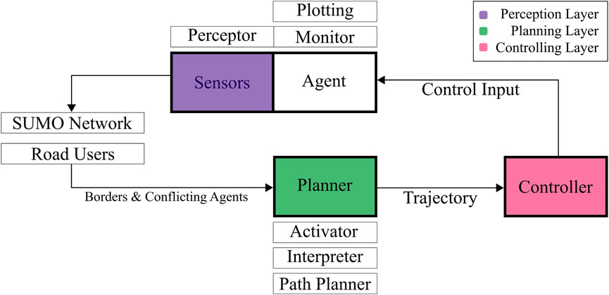
FIGURE 2. The developed Controlling Unit layout of the autonomous agent.

Algorithm 1. The main control loop of the autonomous agent.

1 initialize()

2 while not arrived do

3 Perceptor.find_conflicting_agents();

4 PathPlanner.get_path() → path;

5 Controller.make_trajectory() → trajectory;

6 for i in range(0, len(trajectory)) do

7 Simulator.traci_step()

8 if check_for_arrival() then

9 plot_results();

10 arrived = True;

11 break;

12 end

13 Activator.conflict_agent_speed_changed();

14 if Activator.agent_finished_overtaking() then

15 break

16 end

17 if Activator.agent_passed_stopping_vehicle() then

18. break

19 end

20 Perceptor.plot_and_sensor_update();

21 Perceptor.find_conflicting_agents();

22 if Interpreter.is_enabled then

23 if Interpreter.check_for_conflict() then

24 break

25 end

26 if Interpreter.check_for_junction_control() then

27 break;

28 end

29 if Activator.acceleration_changed() then

30 break;

31 end

32 end

33 if Perceptor.junction_in_view() then

34 break;

35 end

36 if overtaking_enabled then

37 if Interpreter.check_for_overtaking() then

38 break;

39 end

40 end

41 end

42 end

2.3 Sensors and perceptor

The autonomous agent’s path planning relies on the recognition of the lane borders along its route and the detection of other simulated agents. To sense its environment, the agent is fitted with a front camera model and a forward facing LiDAR sensor model. In reality, autonomous vehicles are fitted with many more perception hardware and sensors, however, this work only serves as a proof of concept and limits the sensor setup to a minimum in order to guarantee full functionality while saving computing cost. It is however possible for future applications to add additional sensors in different positions across the vehicle model and assess its performance with different sensor setups. To add the different sensors and cameras to the model, a local coordinate system, based on the agent’s back right corner is first defined.

The LiDAR is modeled as a collection of rays with a set length joined to a sensor cone of a certain reach, coverage, and covering angle. A higher coverage results in a greater number of rays assigned to the sensor. To simulate the functionality of a radar, the frequency of the agent’s sensor can also be set. For each sensor ray, the intersection point with the closest road border is calculated, set as the ray’s endpoint, and identified as a definite road border data point. The algorithm principle is given by Algorithm 2. During the time of active AV control, all this data gathered by the LiDAR sensor is recorded by the Controlling Unit’s Data Monitor (see Figure 2). In order to determine the agent’s final path, the data points are labeled as either being on the left or right border of the agent’s current driving lane. Therefore, the data points are checked beginning with the point closest to the agent and then moving along the data points always finding the closest neighbor to the current point. This procedure is repeated until the distance to the closest neighbor exceeds the current lane width. Once this criterion is met, the second closest, not-yet-labeled point to the agent’s position is found and then processed as in the previous step, again until the distance exceeds the lane width. The high frequency of the sensor updates (given by the time step in SUMO, or, if set, the sensor’s frequency) ensures sufficient input for the path planning process, even though the evaluation logic skips some data points. Figure 4 shows the described logic showing color-coded outputs.

Algorithm 2. The Border Derivation Algorithm

1 border = list(closest_pt);

2 new_closest = None;

3 pt_to_remove = 0;

4 while sensor_data_pts is not empty do

5 min_dist = inf;

6 closest_pt = border[-1];

7 for i in range(0, len(sensor_data_pts)) do

8 current_dist = dist(closest_pt, sensor_data_pts[i]);

9 if current_dist $<$ min_dist then

10 new_closest = sensor_data_pts[i] min_dist = current_dist;

11 pt_to_remove = i;

12 end

13 if min_dist ≥ lane_width then

14 break;

15 end

16 border.append(new_closest);

17 sensor_data_pts.remove(pt_to_remove)

18 end

19 end

20 return border;

The Camera Sensor is modeled as a cone represented by a polygon, basically determining the agent’s field of view. Every object that falls within the field of view polygon will be recognized by the agent and considered in the further planning process. The camera’s specifications assume the ability to recognize nearby intersections, as well as the position, speed, and orientation at the current time step of nearby agents falling inside the cone of view. The sensor layout is presented in Figure 3 and a detailed example of the sensor setup in operation in Figure 4.

FIGURE 3

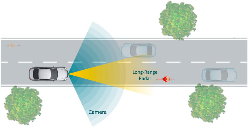
FIGURE 3. The sensor layout of the autonomous agent used in this work.

FIGURE 4

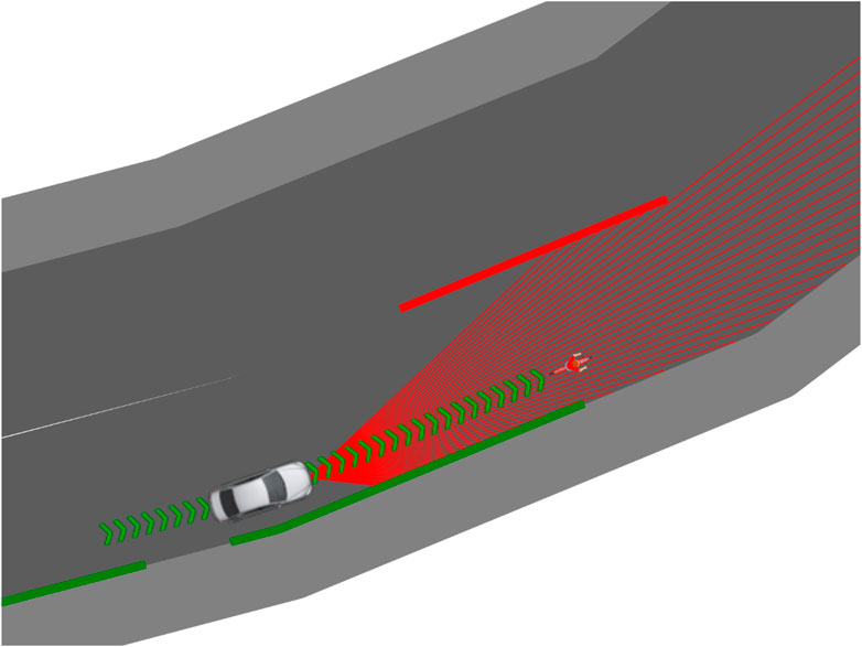
FIGURE 4. The visualisation of the sensor working principle including the projected trajectory. The thin red lines represent the LiDAR’s recognition rays, with the thick red and green lines showing the derived left and right lane border and, ultimately, the proposed driving path given by the green chevrons.

The Perceptor proceeds to classify all detected agents inside the field of view of the sensors so that the autonomous agent can react to them in the appropriate order. The classification developed in the course of this work is based on the conflicting vehicle’s position and its orientation. It groups the detected agents into the following sets:

• Agents in View: all agents, which are currently inside the field of view

• Aligned Agents: all agents facing the same direction as the autonomous agent

• Oncoming Agents: all agents facing the opposite direction as the autonomous agent

• Agents to Yield: all agents approaching the autonomous agent from the right and, therefore, having the right of way, e.g. at intersections

• Minor Agents: agents, which are in the field of view, however, their role in the current traffic situation is rather minor due to, for example, their distance from the autonomous agent or because they are approaching from the left and, therefore, must yield to the autonomous agent

In order to keep a certain flexibility in assigning the conflict vehicle to a specific group, a deviation angle Δϕ is introduced, so that vehicles traveling in the autonomous agent’s direction or in a direction within a user specified interval will still be considered an aligned agent. The same principle is used for the other groups. All these sets are then sorted in an ascending manner according to the conflicting agent’s distance to the autonomous agent. The logic is presented in Figure 5 given by Algorithm 3.

FIGURE 5

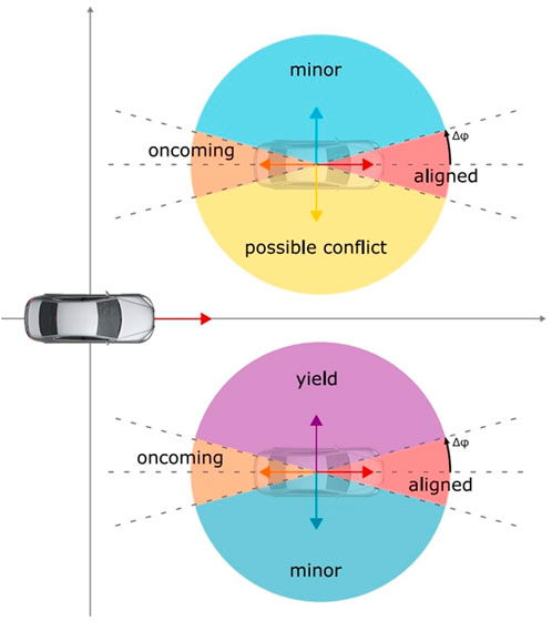
FIGURE 5. The sorting principle of conflicting agents.

Algorithm 3. Get Agent Role Algorithm.

1 move_conflict_agent_to_origin();

2 rotate_conflict_agent_to_zero();

3 if conflict_angle $<$ 0 then

4 conflict_angle += 2 *π;

//Takes care of negative angles

5 end

6 if eps ≤ conflict_angle ≤ π - eps then

7 if conflict_agent_left_of_av_agent then

8 conflict_role = minor;

9 end

10 else

11 conflict_role = yield;

12 end

13 end

14 else if π - eps ≤ conflict_angle ≤ π + eps then

15 conflict_role = oncoming;

16 end

17 else if π + eps ≤ conflict_angle $<\pi$ - eps then

18 conflict_role = minor;

19 end

20 else

21 conflict_role = aligned;

22 end

2.4 Interpreter

The Interpreter can be seen as the autonomous agent’s brain. After the Perceptor recorded the agent’s surrounding area, the Interpreter assesses the current situation based on the gathered input data. Figure 6 presents the decision tree of the Interpreter, with the yellow arrow illustrating the importance hierarchy of the various conflict checks. In comparison to existing car following models, the Interpreter also takes into account other simulated vehicles that are not directly in a leading position compared to the autonomous agent, as well as handling intersections and overtaking maneuvers.

FIGURE 6

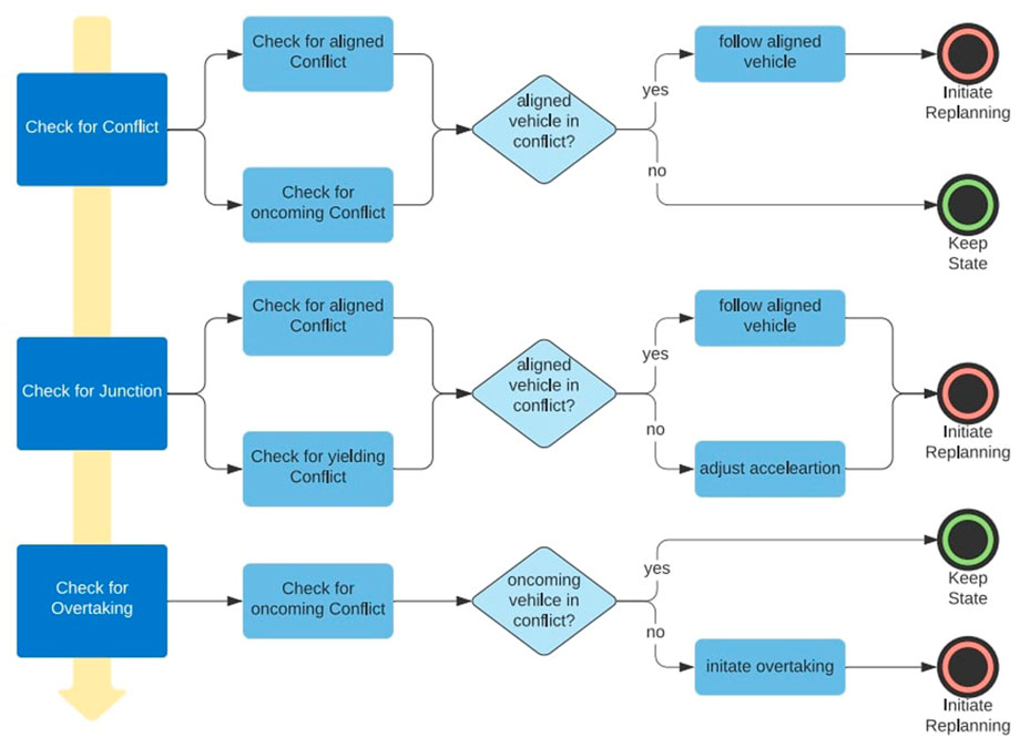
FIGURE 6. The developed Controlling Unit logic of the autonomous agent.

The first check performed by the controlling unit is for imminent conflicts. The leading vehicle of the autonomous agent will always be the critical vehicle to react to in every traffic situation. Therefore, the check and ultimately the reaction to a conflicting aligned vehicle (conflict meaning within a certain distance to the autonomous agent) always wins over any decision made based on other conflicting vehicles. Obviously, the control value affected by a leading vehicle is the acceleration, or deceleration α_ego in case of a vehicle traveling at a lower velocity than the autonomous agent. The autonomous agent needs to always maintain a minimum gap x_min to the leading vehicle and aims for the same speed as the leading traffic participant. Since this paper focuses on the interaction with bicyclists this is a viable speed target and exceeding speed limits is not relevant (However, to address speed limits, the autonomous agent model is also configurable with a maximum speed limit). A re-planning of the autonomous agent’s path will then take place whenever the leading vehicle’s speed changes. Therefore, for the re-planning step, one can assume α_conflict = 0. This results in the autonomous agent’s change of position based on time and its change in velocity based on time specified by the following equations, which are all based on the fundamental laws of movement given in Gerlough and Huber (1975):

$\mathrm{\Delta }x\left(t\right)=x_{\mathit{conflict}}\left(t\right)+v_{\mathit{conflict}}\left(t\right)\ast t-v_{\mathit{ego}}\left(t\right)\ast t-\frac{1}{2}\ast {\alpha }_{\mathit{ego}}\left(t\right)\ast t^2(1)$

$\mathrm{\Delta }v\left(t\right)=v_{\mathit{conflict}}\left(t\right)+v_{\mathit{ego}}\left(t\right)\ast t-{\alpha }_{\mathit{ego}}\left(t\right)\ast t(2)$

This equation system has a unique solution for the predicted time gap t_mingap it takes for the autonomous agent to reach the minimum tolerable distance x_min−x_conflict,i to the leading agent and the respective acceleration α_ego,i given the current agent states, resulting in the following set of equations for any given time step i:

$t_{\mathit{mingap,i}}=\frac{2\ast \left(x_{\mathit{min}}-x_{\mathit{conflict,i}}\right)}{v_{\mathit{conflict,i}}-v_{\mathit{ego,i}}}(3)$

$a_{\mathit{ego,i}}=\frac{v_{\mathit{conflict,i}}-v_{\mathit{ego,i}}}{t_{\mathit{mingap,i}}}(4)$

In a second step, the check for an upcoming intersection is performed. This control module adjusts the agent’s control in the vicinity of intersections. In case of a nearby intersection, the presence of an agent with right-of-way, and the absence of a leading agent, the autonomous agent’s acceleration or deceleration a_ego will be adjusted in such a way that the time to arrival t_ego,arr is outside the time interval defined by the arrival time of the conflicting agent t_conflict,arr and a user-defined safety time gap t_safety. Given a nearby intersection and an agent with right-of-way, the autonomous agent’s time to arrival t_ego,arr,i at any given time step i can be calculated as follows:

$t_{\mathit{ego,arr,i}}=\frac{-v_{\mathit{ego,i}}\pm \sqrt{\left(v_{\mathit{ego,i}}^2+2\ast {\alpha }_{\mathit{ego,i}}\ast \left|x_{\mathit{ego,i}}-x_{\mathit{intersection}}\right|\right)}}{{\alpha }_{\mathit{ego,i}}}(5)$

Assuming an acceleration a_conflict = 0 for the conflicting agent at the intersection, the arrival time of the agent to yield is:

$t_{\mathit{conflict,arr,i}}=\frac{\left|x_{\mathit{conflict,i}}-x_{\mathit{intersection}}\right|\left.\right)}{v_{\mathit{conflict,i}}}(6)$

Subsequently, an adjusted acceleration a_ego,i+1 for the autonomous agent is necessary, if the following criterion is met:

$\left|t_{\mathit{conflict,arr,i}}-t_{\mathit{ego,arr,i}}\right|\le t_{\mathit{safety}}(7)$

If the autonomous agent’s predicted arrival time is prior to the conflicting arrival time, the desired arrival time t_des,arr,i is given by:

$t_{\mathit{des,arr,i}}=t_{\mathit{conflict,arr,i}}-t_{\mathit{safety}}(8)$

Unless the autonomous agent’s predicted arrival time is later than the conflicting arrival time, in which case it is given by:

$t_{\mathit{des,arr,i}}=t_{\mathit{conflict,arr,i}}+t_{\mathit{safety}}(9)$

If the autonomous agent’s predicted arrival time is prior to the conflict’s arrival time, an acceleration is necessary—or, in the case of a later arrival time, a deceleration—which is calculated by:

$a_{\mathit{ego,i+1}}=\frac{2\ast \left(\left|x_{\mathit{ego,i}}-x_{\mathit{intersection}}\right|\right)-v_{\mathit{ego,i}}\ast t_{\mathit{des,arr,i}}}{t_{\mathit{des,arr,i}}^2}(10)$

This logic allows for a continuous stream of traffic without the necessity to stop at intersections possibly causing delays and traffic jams in upstream traffic.

Finally the check for overtaking is performed. The overtaking logic implemented in this work imitates the driver’s behavior in a real traffic situation. Provided a certain decision and sight distance to the leading vehicle in order to evaluate the overtaking situation, the Interpreter considers oncoming vehicles and upcoming intersections. To guarantee a safe manoeuvre, the autonomous agent must finish its overtaking with a safety gap x_safety,1 to the vehicle to be overtaken and an additional safety gap x_safety,2 to the oncoming vehicle, in order not to affect other traffic. Further, the maneuver must be finished before reaching a distance of x_min of any downstream intersection. First, the time necessary for an overtaking maneuver t_m is calculated at the overtaking maneuver initiation time step i = 0:

$\mathrm{\Delta }v=v_{\mathit{ego,0}}-v_{\mathit{conflict,0}}(11)$

$t_m=\frac{\mathrm{\Delta }v\pm \sqrt{{\left(\mathrm{\Delta }v\right)}^2+2\ast a_{\mathit{ego}}\ast \left(\left|x_{\mathit{ego,0}}-x_{\mathit{conflict,0}}\right|\right)+x_{\mathit{safety,1}}+L_{\mathit{ego}}}}{-{\alpha }_{\mathit{ego,max}}}(12)$

The necessary distance for the overtaking move is derived based on the time t_m and the maximum acceleration of the autonomous agent α_ego,max and given by the following equation:

$x_m=x_{\mathit{ego}}\ast t_m+\frac{1}{2}\ast {\alpha }_{\mathit{ego,max}}\ast t_m^2(13)$

For the above stated safety reasons, the overtaking move will only be initiated, if the following criterion is met:

$\mathrm{\Delta }x\left(t_m\right)\stackrel{!}{=}\left(\left|x_{\mathit{ego,0}}-x_{\mathit{oncoming,0}}\right|\right)+v_{\mathit{oncoming}}\ast t_m-v_{\mathit{ego}}\ast t-\frac{1}{2}\ast {\alpha }_{\mathit{ego,max}}\ast t_m^2(14)$

In order to avoid unnecessary re-planning cycles, the Interpreter is fitted with an additional upstream Activator. The Activator tracks the agent’s acceleration α_ego,i−1 in the previous time step i, as well as the current critical conflict vehicle, its speed v_{conflict,i−1}, and the current traffic situation to be handled. Based on these parameters, the Interpreter can be switched off, so that the agent maintains its current driving state until a certain threshold in the change of the environment parameters is exceeded.

2.5 Path planner

The Path Planner’s task is to derive a path considering the vehicle dynamic constraints based on the agent’s surroundings such as intersections, obstacles, and most importantly lane borders. In a first step, it is necessary to derive the desired path from the start to the end position within the given road network. This initial control is equivalent to standard satellite navigation, which considers the entire road network and returns the shortest path from start to goal resulting in an ordered list of network nodes and edges to be passed. Planning is based on an A* path finding algorithm presented in Koubaa et al. (2018), which is an extension of Dijkstra’s Algorithm, but achieves better performance with respect to time.

While driving, the agent’s trajectory is calculated as the center-line using the left and right lane borders, which are recognized by the Perceptor, as reference. These functions assume no obstacles for the current lane such as vehicles parked along the side of the road. The path itself is a poly-line, not yet containing specific controlling information such as speed, time-based agent placement, or orientation. The actual driving behavior will be derived subsequently by the Controller.

In order to decouple the agent’s path from a lane—i.e., in order to pass a stopping vehicle due to oncoming traffic—an RRT* path planning algorithm with a subsequent Dubins Paths optimization has been proposed. Although it is possible to directly implement the agent’s motion constraints within the RRT* planning, the resulting path turns out very curvy (without optimization) and does not produce a feasible solution to the problem. Besides, it makes RRT* a lot more computationally expensive compared to using simple straight edges. Therefore, an initial RRT* motion planning without differential constraints is used in order to explore the configuration space C for a set number of iterations N or until a path to the target position z_end (the end of the intersection) is found. In a second step, the shortest path from the agent’s position to the end of the intersection is split at z_mid in a 1:2 ratio, defined as the ratio of the number of nodes along the target path from the middle node to the target node and the number of nodes from the start node to the middle node calculated as the nearest integer. This results in two consecutive segments which are then converted into two Dubins curves—comprising the actual desired path—passing the obstructing vehicle LaValle (2006). Despite the fact, that usually cloothoids are used in traffic engineering, this paper uses Dubins curves instead in order to provide a proof-of-concept while maintaining implementation simplicity. However, cloothoids can easily replace the current paths in further research. The minimum turning radius used for the resulting Dubins curves r_ego,min can be calculated, ignoring traversal jerk and maximum cornering acceleration, based on the Ackermann steering model and is dependent of the maximum steering angle ϕ_ego,max given by the following equations Lavacs (2006):

$r_{\mathit{ego,min}}=\frac{L_{\mathit{ego}}}{\mathit{sin}\left({\varphi }_{\mathit{ego,max}}\right)}(15)$

Resulting in a maximum curvature of:

$c_{\mathit{ego,max}}=\frac{\mathit{sin}\left({\varphi }_{\mathit{ego,max}}\right)}{L_{\mathit{ego}}}(16)$

The end result is shown in Figure 7. The Dubins paths implementation used in this work is taken from Sakai et al. (2018). A main advantage of the path planner is that the proposed methodology enables lane-free motion of the simulated autonomous agent in comparison to the existing models used in SUMO, where the lateral movement of vehicles is lane-based, typically simulated through discrete lane choice models or through the resolution of a traffic lane into sub-lanes Semrau and Erdmann (2016).

FIGURE 7

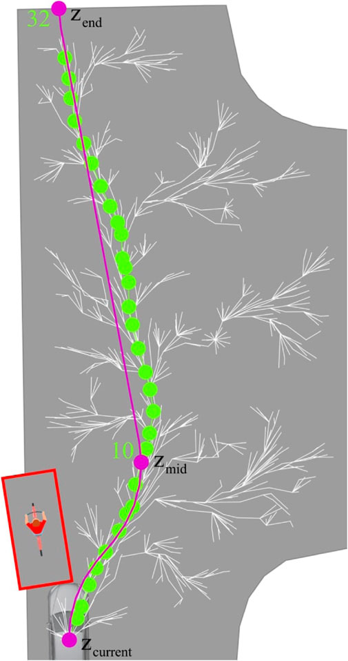
FIGURE 7. Intersection passing path planning results combining RRT* with dubins path. The green path represents the path, chosen by the RRT* algorithm. The purple curve then gives the optimsed dubins path, whilst the white edges show the complete RRT* output.

2.6 Controlling

After the current traffic situation has been evaluated by the Interpreter and an appropriate path has been generated by the Path Planner, the Controller is responsible for creating the final trajectory for the upcoming time steps t_i: ∈ [0, T]. It consists of the actual positions x_i(t) following the given path, the respective orientation θ_i(t), and the anticipated speed v_i(t). The control logic is based on the acceleration determined by the Interpreter for the current traffic situation and, additionally, the engine’s limitations, such as the maximum acceleration and speed. The evaluation points x_i(t) and orientations θ_i(t) are indicated by markers, which are colour-coded based on the respective speed and can be annotated by the velocity for better examination.

2.7 Comparison of the agent’s behavior to the existing driving models

In order to assess the driving behavior of the autonomous vehicle model in response to interactions with bicyclists, its trajectory will be compared to some of the existing driving models already implemented in SUMO. Therefore, in the developed scenarios the AV was replaced by agents controlled through SUMO using the following already implemented CFMs:

• The Car Following Model Wiedemann 99, 10-Parameter version as implemented in SUMO (Lopez et al., 2018).

• The Krauss Model with some modifications, which is the default model used in SUMO Krauss et al. (1997).

• The Intelligent Driver Model (IDM) Treiber and Kesting (2013).

The CFMs are coupled with the SUMO sub-lane model Semrau and Erdmann (2016). For the agents controlled by the three models defined in SUMO, corresponding vehicle types (vType) are created, which correspond in their properties to those of the autonomous agent. Arbitrary scenarios can therefore be simulated without using the autonomous vehicle control logic. Since both the behavior of the autonomous agent and the agents controlled by SUMO follow the default logic and the parameters of the critical agent have not been changed, making the tests deterministic, it was sufficient for the evaluation of the autonomous vehicle model to run through each test scenario only once. Further, this work is intended to develop a general autonomous vehicle framework to be used for further research and tests, so the proposed test scenarios only evaluate the basic functions of an autonomous vehicle. The behavior of the different agents is evaluated based on the scenario using key traffic parameters such as the average speed, maximum acceleration, maximum deceleration, waiting time, and time to collision Hou et al. (2014). The TTC is a defined as:

$TTC=\frac{|x_{\mathit{ego}}\left(t\right)-x_{\mathit{conflict}}\left(t\right)|}{{\dot{x}}_{\mathit{ego}}\left(t\right)-{\dot{x}}_{\mathit{conflict}}\left(t\right)}(17)$

The required time to collision TTC_req defined by the minimum safety gap, the current speed and acceleration

$TT{C}_{\mathit{req}}=\frac{\mathrm{\Delta }v\pm \sqrt{\mathrm{\Delta }{v}^2+2\ast \left({\alpha }_{\mathit{ego,i}}-{\alpha }_{\mathit{conflict,i}}\right)\ast safety\text{\_}gap}}{{\alpha }_{\mathit{ego,i}}-{\alpha }_{\mathit{conflict,i}}}(18)$

with

$\mathrm{\Delta }v=v_{\mathit{ego,i}}-v_{\mathit{conflict,i}}(19)$

Given the current speed, a maximum braking deceleration is specified by SUMO Lopez et al. (2018):

${\alpha }_{\mathit{brake}}=-7.5m/s^2(20)$

The Time To Stop (TTS) is then a function of:

$TTS=\frac{-v_{\mathit{ego}}}{{\alpha }_{\mathit{brake}}}(21)$

2.7.1 The bicycle simulator dataset

In order to assess the proposed autonomous vehicle model and compare its performance to existing models, trajectories gathered using the bicycle simulator described in Keler et al. (2018) are used. All the non-autonomous agents in this study are controlled based on these trajectories and not by any specific CFM. The bicyclist trajectories were gathered as part of a previous bicycle simulator study with 30 participants per scenario (This does not suffice for statistic significance, however, it gives a good starting test for a initial model), where test subjects were asked to perform common bicyclist maneuvers in mixed traffic conditions with motor vehicles. Three scenarios were examined for left turns, two scenarios for the crossing, and one scenario for right turns at an non-signalized intersection. Additional scenarios included the test subjects performing lane changing maneuvers along a road section and crossing a roundabout. These scenarios were specifically chosen in order to account for frequent urban traffic situations. The speed limit on all streets was set to 30 km/h. For the purposes of this work and to account for all the simulator data, the autonomous agent’s control logic has been tested with an average trajectory based on all thirty test subjects of each specific scenario. This has the advantage that noise from the orientation data points, which was quite common, could be eliminated. A correct and especially continuous orientation is very important, as the autonomous agent’s interpretation ability relies on accurate agent orientation. Key scenarios are thoroughly described in the next subsections.

2.7.2 Scenario 1—Simple following

The first scenario simulates a simple bicycle following scenario without any turning or overtaking desire by the involved agents. Both agents are simply moving along a straight road segment without any other vehicles to yield to or obstacles. When placed at their initial positions, the distance between the autonomous agent and the bicyclist is 120m. This is to ensure that the autonomous agent starts driving freely, not being influenced by the critical agent, since it is not within the field of view Figure 8A.

FIGURE 8

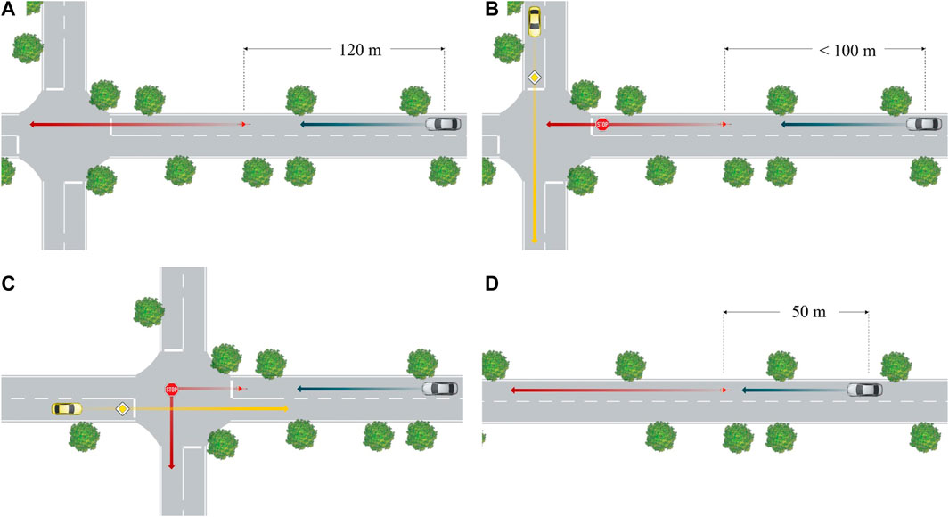
FIGURE 8. (A) Scenario 1- Simple Following, (B) scenario 2—Advanced Following, (C) scenario 3—Intersection Passing, (D) scenario 4—Overtaking.

2.7.3 Scenario 2—Advanced following

The goal of scenario 2 is to examine the autonomous agent’s behavior when interacting with a stopping leading critical bicycle agent. Unlike the previous scenario, the bicycle agent starts already within the autonomous agent’s field of view. Until reaching the minimum gap, the autonomous agent simply follows the leading critical agent until it comes to a stop. In order to simulate more realistic driving behavior, additionally to the safety gap, an absolute minimum gap is introduced, which results in a final approach up to this distance when the leading critical agent stops. For varying tests, the critical agent’s stopping position as well as the anticipated stopping time can be defined, which has been set to 10s in this example (see Figure 8B).

2.7.4 Scenario 3—Junction passing

Scenario 3 requires the most advanced planning effort for the autonomous agent’s driving behavior. The simulation setup is again based on a leading bicyclist and an additional intersecting agent traveling in the opposite direction of the autonomous agent. However, the bicyclist’s desire to make a left turn in combination with the oncoming traffic leads to the critical agent stopping in the middle of the intersection, which is a very common scenario occurring at non-signalized intersections (see Figure 8C). It is important to mention that the stopping of the preceding agent in both scenario 2 and scenario 3 was modeled using a reference coordinate, which was chose to be a fixed coordinate just before entering the intersecting lane representing the typical location a left-turning vehicle or cyclist would stop in order to let oncoming traffic pass. When passing this reference coordinate, the simulation causes the preceding agent to rather suddenly stop without taking into account physical limits such as realistic negative acceleration. As a result, the braking acceleration of the preceding vehicle reaches very high values as can be seen in Figure 9B and Figure 10B. Even if the stopping behavior of the bicyclist is therefore unrealistic, its implementation fulfills its purpose, since the scenario task for the autonomous agent is to pass a stationary obstacle at an intersection. The reason why and how the obstacle stopped is not important to evaluate the proposed autonomous agent model. The junction passing itself is modeled using an RRT* algorithm excluding the bicyclists extended by a certain safety distance from the configuration space. The resulting path is optimized using dubins paths and in the following split into two sections in a 1:2 ratio in order to guarantee smooth driving behavior. The logic is shown in Algorithm 4.

FIGURE 9

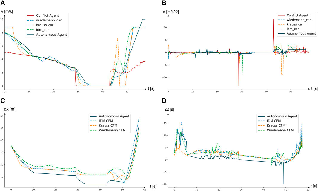
FIGURE 9. (A) Resulting speed profiles for scenario 2, (B) resulting acceleration and deceleration profiles for scenario 2, (C) showing the distance to the leading agent for scenario 2, (D) showing the difference between the actual TTC and TTC_req defined by the given minimum safety distance to the leading agent for scenario 2.

FIGURE 10

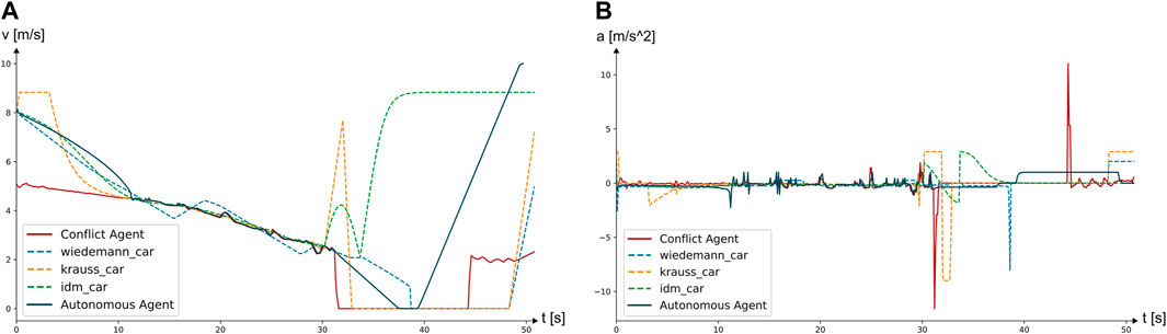
FIGURE 10. (A) Resulting speed profiles for scenario 3, (B) resulting acceleration and deceleration profiles for scenario 3.

Algorithm 4. Junction Vehicle Passing Algorithm.

1 InitializeRRT(C_f, C_b, z_current);

2 z_end = RRTPlanning(N);

3 RenumberTargetPath(z_end);

4 z_mid = GetNodeByNumber(int(z_end.nbr/3));

5 segment₁ = DubinsPath(z_current, z_mid, c = c_ego,max);

6 segment₂ = DubinsPath(z_mid, z_end, c = c_ego,max);

7 path = Join(segment₁, segment₂);

8 return path

2.7.5 Scenario 4—Overtaking

Since in urban traffic situations, bicyclists and vehicles are often travelling at different speeds, overtaking maneuvers are quite common. A maximum overtaking speed and acceleration for the autonomous agent have already been defined. The maximum speed is extended to 15m/s and the maximum acceleration to 2m/s² respectively. The scenario setup is presented in Figure 8D.

3 Results

3.1 Testing setup

All tests were run under Windows 10 Pro N Version 1903 using SUMO build v1_3_1+0841-0db23d23c1 and a machine with the following hardware specifications:

• Processor: Intel Core i7-6700K CPU @ 4.00GHz

• Memory: 16.0 GB

• GPU: GeForce GTX 1070 GPU @ 8 GB GDDR5

3.2 Scenario 1—Simple following

The main goal of the simple following scenario is to drive as close to the desired minimum gap and to reach a maximum average velocity throughout the simulation. Results show that the autonomous vehicle model drove at maximum average speed in comparison to the other CFMs (see Figure 11A) while maintaining relatively low maximum acceleration and deceleration values, indicating a smooth driving (see Figure 11B). In fact, the other CFMs show high deflections in acceleration especially when reaching a shorter distance to the leading agent. Figure 11D shows TTC−TTC_req for the different vehicle models, which should be as close to zero as possible when reaching the minimum allowed gap. The autonomous agent successfully maintains a stable minimum distance to the leading vehicle.The constant switch between positive and negative acceleration, when reaching the minimum gap is due to the agents controller trying to adjust to the leading bicyclist’s slightly changing speed.

FIGURE 11

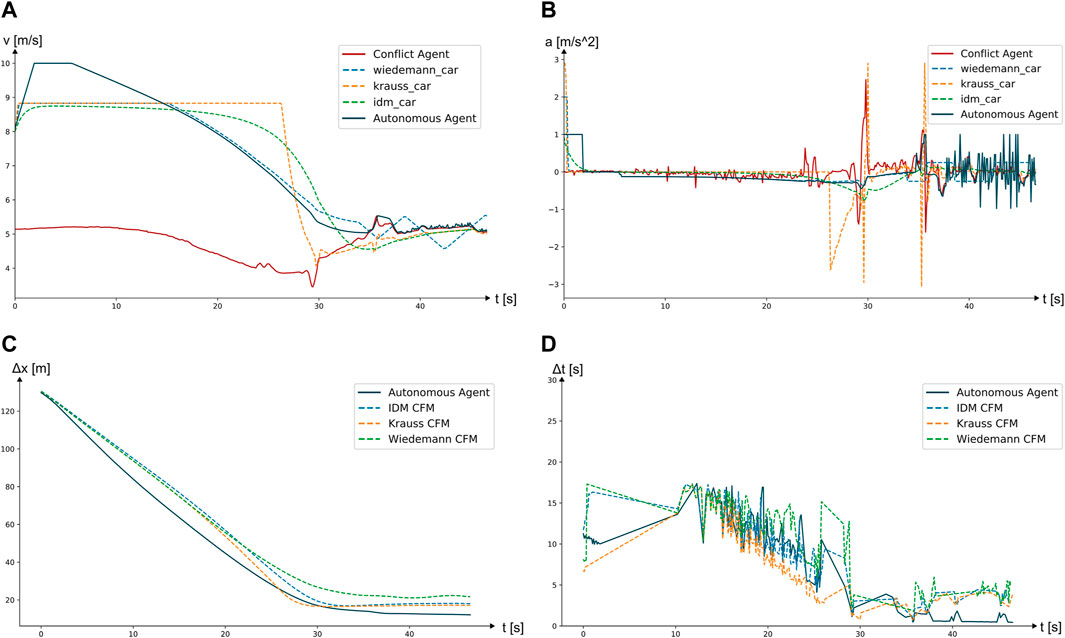
FIGURE 11. (A) Resulting speed profiles for scenario 1, (B) resulting acceleration and deceleration profiles for scenario 1, (C) showing the distance to the leading agent for scenario 1, (D) showing the difference between the actual TTC and TTC_req defined by the given minimum safety distance to the leading agent for scenario 1.

3.3 Scenario 2—Advanced following

Figure 9A shows the leading critical agent stopping at around 28s, resulting in the autonomous agent reaching the absolute minimum gap. The existing CFMs, although given the same safety gap as the autonomous agent, do not drive as closely to the minimum gap as possible, showing deviations almost twice the defined value (see Figure 9B). However, the speeds are equally accurate to the bicyclist’s speed for all the CFMs, shown in Figure 9C.

When comparing the results of the autonomous agent to the existing models it becomes clear, that, even though existing models also perform a second approach upon the leading vehicle’s stop, they do not drive closer to the critical agent than the minimum safety gap, resulting in rather unrealistic driving behavior. This ultimately leads to greater deviations of TTC from TTC_req (See Figure 9D). A drop in the autonomous agent’s TTC−TTC_req can also be found in Figure 9D. This is due to the fact, that the autonomous agent has two safety gaps defined: A minimum safety gap, when driving in a fluid traffic situation and and absolute safety gap, when approaching and ultimately stopping behind a leading stopped traffic participant. The absolute safety gap, however, leads to a violation of the minimum required time to collision. After all, this does not lead to any dangerous situations and mimics realistic driving behavior.

3.4 Scenario 3—Intersection passing

In this scenario, the stopping agent produces comparable deflections to the agent’s acceleration in scenario 2. Its stopping position is denoted by a red dot in Figure 10A. Unlike the other SUMO models, after entering the intersection and reaching its maximum tolerable stopping time, the autonomous agent begins a right-hand side overtaking maneuver at the intersection. This behavior is enabled by the path-planning module of the autonomous agent, which enables lane-free movement, in contrast to those of agents simulated by the simulation software, whose movement is limited to the available lane space. The simulation ends before the critical agent has fully left the intersection, hence the SUMO models do not continue their driving after they have come to a stop. Additionally as observed in Figure 10C and Figure 12, the IDM model fails to stop and passes through the simulated bicyclist. However, even the other SUMO CFMs seem to struggle with this scenario, shown by partly high deflections in their accelerations in Figure 10B.

FIGURE 12

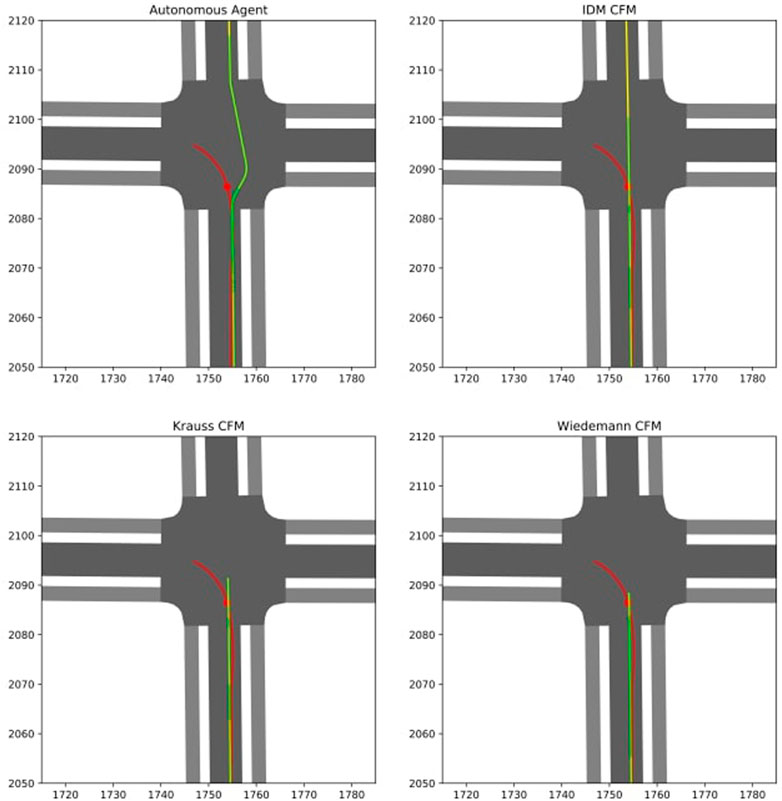
FIGURE 12. The trajectories of the autonomous agent in comparison to the other car models scenario 3.

Regarding the total waiting times of the various CFMs, the AV model results in the lowest waiting time (2s), due to its ability to pass a stopped agent in comparison to Krauss (15.5s) and Wiedemann (9.7s). Although resulting in the lowest waiting time of (0s), the IDM agent’s behavior is not considered correct, as it leads to a collision with the stopping critical agent. Another interesting observation is the deflection in the Krauss agent’s speed in Figure 10A at around 32s, which shows that the CFM first interprets the obstacle as negligible, but quickly after changes its decision and performs a stop as well, resulting in strong braking.

3.5 Scenario 4—Overtaking

Since scenario 4 is also based on a straight road section, the highest possible average speed within the permissible maximum speed while reaching the target position as fast as possible is desirable. Due to a lack of oncoming traffic, an overtaking maneuver is the most logical consequence for the agents after they have reached the leading critical agent. However, none of the SUMO CFMs is capable of such a maneuver if it involves entering the oncoming lane. Thus, the SUMO agents simply follow the leading critical agent, maintaining a similar speed and safety distance, as shown in Figures 13A,B. On the contrary, it is possible for the autonomous agent to perform an overtaking maneuver according to the proposed control logic, even when using the opposite lane. This results in a great difference in the autonomous agent’s trajectory in comparison to the other vehicle models. Unlike the other scenarios, the CFMs perform fairly well in regards to their acceleration, shown in Figure 13B, resulting in a maximum deceleration of −2.9 m/s², which is the defined maximum braking deceleration for the SUMO agents not leading to uncomfortable driving behavior.

FIGURE 13

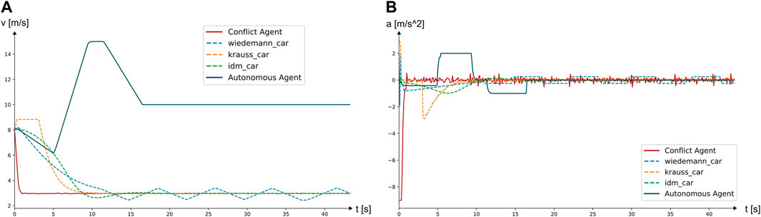
FIGURE 13. (A) Resulting speed profiles for scenario 4, (B) resulting acceleration and deceleration profiles for scenario 4.

4 Discussion

4.1 Limitations

The following design of a car following model primarily assumes correct driving behavior of other road users. Scenarios in which this behavior is violated or randomness, such as sensor failure or unnatural bike-riding behavior, were not considered in the concept design. Furthermore, individual modeling steps, such as that of a stopping preceding vehicle, lead to partially unrealistic driving behavior of the preceding vehicle due to their implementation. This limitation was accepted, however, in order to test certain functionalities of the developed car following model. Since the underlying study was based on bicyclists as interaction vehicles, such were also used as control vehicles in the design of the car following model. Nevertheless, all design concepts work with any type of control vehicle. A further limitation regarding the autonomous vehicle model is the simplification to a one-dimensional driving model resulting in the neglection of traversal jerk such as lateral acceleration, which becomes particularly important in the context of the path optimization used due to the Dubins curves. This leads to a simplified cornering behavior throughout the conducted simulations. Performance optimization was also not considered when implementing the autonomous agent’s logic. Therefore, all simulations were performed on a single machine, which led to performance interference of the running simulation with the autonomous agent calculations. However, looking at Figure 14 and Figure 15 show the duration of the control unit’s calculation duration against the threshold of 0.1 s, which was the duration of one simulation time step within SUMO. This illustrates that no considerable input lag was introduced by the control logic apart from the path planning in scenario 3, which should be improved considering performance in further research.

FIGURE 14

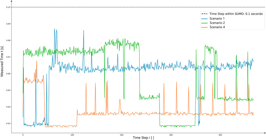
FIGURE 14. Showing the duration of the different controlling steps during the simulation for scenarios 1, 2, and 4 against the time step duration threshold within SUMO, which was chosen to be 0.1 s.

FIGURE 15

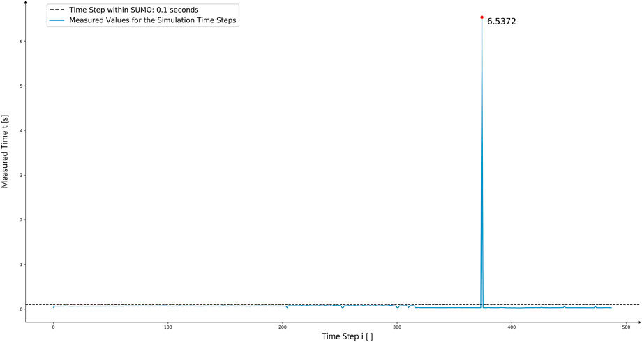
FIGURE 15. Showing the duration of the different controlling steps during the simulation for scenario 3 against the time step duration threshold within SUMO, which was chosen to be 0.1 s.

4.2 Conclusion

In this work, an autonomous vehicle model based on current state of the art in robotics and autonomous vehicle research was presented and evaluated in the microscopic traffic simulation software SUMO for modeling interactions with bicyclists. The vehicle model features a navigation component, which connects to the microscopic traffic simulation software SUMO through a node edge representation and uses an A* path planning algorithm to generate a path from the start to the target destination, returning all the lanes and intersections along the way. To account for more complex driving maneuvers in the presence of bicyclists, such as overtaking and passing, the autonomous agent is further fitted with an RRT* path planner, which generates a path based on a given configuration space (i.e., the intersection area) converting it to a drivable trajectory based on dubins paths, given the limits defined by the vehicle dynamics model. In a second step, an example AV agent was assembled and tested in common traffic simulation scenarios in SUMO. To evaluate the developed model, the scenarios were also simulated with the autonomous agent replaced by vehicles, that use the existing car following models and the sub-lane model already implemented in SUMO. The derived simulation data was compared to resulting speed and acceleration profiles and to various key evaluation parameters specifically related to the respective scenario.

Results show, that the profiles of the autonomous agent match the profiles generated by the existing driving models that are part of SUMO and that the autonomous agent was able to drive much closer to the given thresholds than the agent models defined in SUMO, leading to a more realistic driving behavior, overall reduction in queuing times, and a potentially higher traffic density throughout the network. Additionally, the autonomous agent was able to perform overtaking maneuvers due to the lane-free path planning approach through the combined use of RRT* and dubins paths. Thus, it outperformed the existing SUMO models in simulation scenarios, where the former are limited by the lane-based simulation approach and the junction model limitations in handling such interactions. This is a significant improvement, especially for modeling bicyclist interactions with autonomous vehicles. Also, the autonomous vehicle model achieves significantly more consistent acceleration and speed profiles compared to the existing SUMO CFMs in the presence of a bicyclist, which improves the simulation accuracy and quality.

The highly modular approach in the Controlling Unit’s implementation allows for easy, uncoupled further research regarding the different control components. It is also possible for users to modify the proposed model components by integrating existing methods and developing and testing their own new methods for autonomous vehicle operation and navigation in traffic environments. Given the stable driving in the tested traffic scenarios, an evaluation of the behavior in more complex scenarios, possibly with several conflict agents, would be interesting. Regarding scenario generation, a coupling with Alekszejenkó and Dobrowiecki (2019) seems possible. To make use of the inter-vehicle and network communication, the agent model could be tested in scenarios with several autonomous agents communicating either with each or other with nearby intersections. It would also be interesting to evaluate overall network utilization taking into account autonomous, non-autonomous vehicles, and bicycle traffic. Finally, considering the results of the first two test scenarios, which are mainly defined by the vehicle following behavior, it becomes clear that the vehicle model developed in this work represents a realistic alternative to the CFMs already defined in SUMO. In further research and development work, this logic could therefore possibly be implemented directly in SUMO as a new CFM called Kimarite. The whole source code developed over the course of this work is freely accessible under: https://github.com/FlixFix/Kimarite.

Data availability statement

The datasets presented in this study can be found in online repositories. The names of the repository/repositories and accession number(s) can be found below: https://github.com/FlixFix/Kimarite.

Ethics statement

Written informed consent was obtained from Patrick Malcolm for the publication of any potentially identifiable images or data included in this article.

Author contributions

The authors confirm contribution to the paper as follows: study conception and design: GG and FR, data collection: PM, GG, AK, and FR; analysis and interpretation of results: FR and GG; draft manuscript preparation: GG, PM, FR, and KB. All authors reviewed the results and approved the final version of the manuscript.

Funding

Federal Ministry for Economic Affairs and Energy of Germany (BMWi), based on a decision taken by the German Bundestag, grant number 19A17015B.

Acknowledgments

This work is part of the research project @CITY—Automated Cars and Intelligent Traffic in the City. The project is supported by the Federal Ministry for Economic Affairs and Energy of Germany (BMWi). The authors are solely responsible for the content of this publication.

Conflict of interest

The authors declare that the research was conducted in the absence of any commercial or financial relationships that could be construed as a potential conflict of interest.

Publisher’s note

All claims expressed in this article are solely those of the authors and do not necessarily represent those of their affiliated organizations, or those of the publisher, the editors and the reviewers. Any product that may be evaluated in this article, or claim that may be made by its manufacturer, is not guaranteed or endorsed by the publisher.

References

Alekszejenkó, L., and Dobrowiecki, T. (2019). Sumo based platform for cooperative intelligent automotive agents. EPiC Ser. Comput. 62, 107–123. doi:10.29007/sc13

CrossRef Full Text | Google Scholar

Barceló, J., and Casas, J. (2005). “Dynamic network simulation with aimsun,” in Simulation approaches in transportation analysis (New York, United States: Springer), 57–98.

Google Scholar

Dosovitskiy, A., Ros, G., Codevilla, F., Lopez, A., and Koltun, V. (2017). “CARLA: An open urban driving simulator,” in Conference on Robot Learning (CoRL 2017), Mountain View, United States. arXiv preprint arXiv:1711.03938.

Google Scholar

Fellendorf, M., and Vortisch, P. (2010). “Microscopic traffic flow simulator VISSIM,” in Fundamentals of traffic simulation (New York, United States: Springer), 63–93.

CrossRef Full Text | Google Scholar

Gerlough, D. L., and Huber, M. J. (1975). Traffic flow theory: A monograph. Transportation Research Board, National Research Council.

Google Scholar

Hou, J., List, G. F., and Guo, X. (2014). New algorithms for computing the time-to-collision in freeway traffic simulation models. Comput. Intell. Neurosci. 2014, 1–8. doi:10.1155/2014/761047

PubMed Abstract | CrossRef Full Text | Google Scholar

Keler, A., Kaths, J., Chucholowski, F., Chucholowski, M., Grigoropoulos, G., Spangler, M., et al. (2018). “A bicycle simulator for experiencing microscopic traffic flow simulation in urban environments,” in IEEE Conference on Intelligent Transportation Systems, Proceedings, ITSC, Maui, HI, USA, 04-07 November 2018. doi:10.1109/ITSC.2018.8569576

CrossRef Full Text | Google Scholar

Kogan, D., and Murray, R. (2006). “Optimization-based navigation for the DARPA grand challenge,” in Conference on Decision and Control (CDC).

Google Scholar

Koubaa, A., Bennaceur, H., Chaari, I., Trigui, S., Ammar, A., Sriti, M.-F., et al. (2018). “Introduction to mobile robot path planning,” in Robot path planning and cooperation (New York, United States: Springer), 3–12.

CrossRef Full Text | Google Scholar

Krauss, S., Wagner, P., and Gawron, C. (1997). Metastable states in a microscopic model of traffic flow. Phys. Rev. E - Stat. Phys. Plasmas, Fluids, Relat. Interdiscip. Top. 55, 5597–5602. doi:10.1103/PhysRevE.55.5597

CrossRef Full Text | Google Scholar

Lavacs, H. (2006). “A 2D car physics model based on Ackermann steering,” in Institute of distributed and multimedia systems (Vienna: University of Vienna).

Google Scholar

LaValle, S. M. (2006). Planning algorithms. Cambridge, New York: Cambridge University Press.

Google Scholar

Lopez, P. A., Behrisch, M., Bieker-walz, L., Erdmann, J., Fl, Y.-p., Hilbrich, R., et al. (2018). “Microscopic traffic simulation using SUMO,” in 2018 21st International Conference on Intelligent Transportation Systems (ITSC), Maui, Hawaii, USA, 04-07 November 2018, 2575–2582. doi:10.1109/ITSC.2018.8569938

CrossRef Full Text | Google Scholar

NVIDIA (2019). Virtual reality autonomous vehicle validation platform Silicon Valley: NVIDIA’s GPU Technology Conference (GTC).

Google Scholar

PTV AG (2016). PTV vissim 9. Karlsruhe: PTV, AG.

Google Scholar

Sakai, A., Ingram, D., Dinius, J., Chawla, K., Raffin, A., and Paques, A. (2018). PythonRobotics: A Python code collection of robotics algorithms. arXiv preprint arXiv:1808.10703.

Google Scholar

Semrau, M., and Erdmann, J. (2016). “Simulation framework for testing ADAS in Chinese traffic situations,” in Proceedings of the 2016 SUMO User Conference, Berlin, Germany, May 23–25, 2016

Google Scholar

Treiber, M., and Kesting, A. (2013). Traffic flow dynamics: Data, models and simulation. Berlin, Germany: Springer-Verlag Berlin Heidelberg.

Google Scholar

Wegener, A., Piorkowski, M., Maxim, R., Hellbrück, H., Fischer, S., and Hubaux, J.-P. (2008). “TraCI : An interface for coupling road traffic and network simulators,” in Proceedings of the 11th communications and networking simulation symposium, Ottawa, Canada, April 14 - 17, 2008, 155–163.

Google Scholar