A movement and interaction model for cyclists and other non-lane-based road users

1 Introduction

Road users differ in their size, dynamics, vulnerability, and behavior. Transportation systems in many countries are centered around the requirements of one type of road user: motorists. Road infrastructure is designed and built to serve the drivers of cars and trucks and the traffic rules and regulations ensure efficiency for motorized traffic. The recent revival of utilitarian cycling, innovations in bicycle engineering that have led to an uptake in e-bikes and cargo bicycles, and the introduction of novel micro-mobility devices, such as e-kick scooters, fundamentally transform urban traffic. The lane and rule-based behavioral patterns associated with motor vehicle traffic are becoming less predominant. These new transport modes are smaller, more flexible, and less encapsulated, leading to more diverse movement patterns and more intuitive interactions between road users. However, tools used to plan and evaluate transportation systems, including microscopic traffic simulation, are not yet able to realistically and reliably recreate this emerging urban traffic.

Operational behavior models are mathematical representations of movement and interactions between road users. They are used in microscopic traffic simulation tools such as SUMO (Krajzewicz et al., 2014) and PTV Vissim (Fellendorf and Vortisch, 2010) to realistically advance simulated road users to their goal or along their desired pathway while reacting to other road users and their environment in a realistic way. The road environment is complex and includes static and dynamic, physical and conceptually defined obstacles, traffic rules, and behavioral norms. Although the input is intricate, the output of an operational behavior model is simple: an acceleration vector $a\left(t\right)$ that is generated for each simulated road user in each simulation time step.

In conventional car-following approaches, acceleration is reduced to a scalar quantity in the longitudinal direction of travel. If movement is constrained by a leading road user, longitudinal acceleration (or deceleration) is derived based on the differences in position and speed of the two road users. The lateral position is not considered in this type of model. In simulation visualizations, vehicles are typically shown moving along the center of the driving lane. Over the last 70 years, a wide variety of car-following models have been formulated and calibrated to recreate the flow of motor vehicle traffic under many conditions. In general, one-dimensional movement and interaction approaches based on desired speeds and car-following models are relatively simplistic and can realistically simulate road users whose behavior is governed by lane discipline. The driving lane-based model is shown schematically in Figure 1A.

FIGURE 1

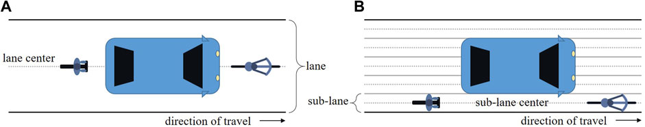
FIGURE 1. Schematic of a lane-based simulation environment (A) and the sub-lane extension (B).

Pedestrians exist on the other side of the spectrum from motor vehicle traffic. Their movement is not controlled by lanes; rather, people traveling by foot move freely on a two-dimensional plane and interact with one another on a more intuitive and less rule-oriented basis. The most common family of models used to simulate this behavior are social force models, the first of which was introduced by Helbing and Molnar (1995). The operating principle of these force models is that the acceleration vector in each time step emerges from the sum of various attractive and repulsive forces experienced by the pedestrian. For example, the destination acts as an attractive force that “pulls” the pedestrian towards it, while repulsive forces “push” the pedestrian away from obstacles and other pedestrians (or other road users). Other forces such as “pull” forces to points of interest or cohesive forces between groups of “friends” can also be included.

The behavior of cyclists and users of many micro-mobility devices falls somewhere in between that of a pedestrian and a motorist. Their movements and interactions are more intuitive and less dependent on lane discipline and traffic rules than motor vehicle drivers. The lack of a vehicle exterior makes it possible for cyclists and micro-mobility users to communicate with other road users in a more human way. Compared to pedestrians, however, these road users have one main axis of movement and are less able to change their velocity at any given moment. Analogous to motor vehicle traffic, engineering measures such as braking distance, minimum turning radius, and the design speed of infrastructure have a meaning for bicycle and micro-mobility traffic that they do not for pedestrian traffic. However, cyclists and micro-mobility users are capable of adjusting their behavior to adapt to the surrounding environment. In busy urban centers or shared spaces, they can slow down and move and interact similarly to a pedestrian. When moving on a road characterized by higher traffic volumes and higher traveling speeds, they can reduce their lateral movement and travel in a mainly longitudinal direction, adhering to the given rules of the road.

Other notable behaviors of cyclists and micro-mobility users include the ability to flexibly adjust their lateral position within a (bicycle) lane to pass other road users (Khan and Raksuntorn, 2001; Yuan et al., 2018), switch between the roadway, cycling infrastructure, and sidewalks (Twaddle and Busch, 2019), and use of unexpected routes to cross intersections (Imbert and Te Brömmelstroet, 2014; Wexler and El-Geneidy, 2017; Lind et al., 2021). It is clear that behavior models developed for the uniform and relatively predictable behavior of motorists can and will not simulate cyclists or users of micro-mobility devices with adequate realism.

How can the movement and interactions of such adaptable road users be modeled? Typically, modifications are made to the simulation environment that allows car-following models to be applied to non-lane-based traffic. In SUMO, a driving or bicycle lane is divided into multiple sub-lanes. Within each sub-lane, the simulated road users move along the one-dimensional lane, their movements controlled by dynamics models and their interactions governed by car-following models (Sekeran et al., 2022). The lateral movement between sub-lanes is controlled using the same or similar models as those used for lane selection and lane change for motor vehicle traffic. The sub-lane approach is illustrated in Figure 1B. Falkenberg et al. (2003) proposed a model in which the longitudinal behavior is governed by a car-following model and the lateral position within a lane is determined by maximizing the Time-To-Collision to leading vehicles/cyclists in the same lane. The lateral and longitudinal models work independently of one another. An adaptation of this model is implemented in PTV Vissim.

These pragmatic approaches allow for the more realistic simulation of cyclists, micro-mobility users, and mixed traffic flows, in which road users pass each other within one lane. However, the flexible nature of non-lane-based traffic, particularly at intersections, or when switching between infrastructures (bicycle lane, sidewalk, and roadway), is not natively replicable (Twaddle et al., 2014a).

Social force models have been formulated for bicycle traffic based on the original concept of pedestrians (see, for example, Li et al. (2011), Li et al. (2021), Liang et al. (2012) and Schönauer et al. (2012)). Although the flexibility of cyclists and their interactions with other road users can be replicated in a realistic way using social force models, the movement must be limited to reflect the dynamics of riding a bicycle. In addition, it can be difficult to replicate tactical behaviors, such as selecting between different types of pathways across an intersection, and using social force alone.

In this paper, a method for linking the modeling paradigms used to simulate motor vehicle traffic (one-dimensional lane-based models) and pedestrian traffic (two-dimensional social force models) is presented. This approach enables the simulation of flexible movement patterns while maintaining a mainly longitudinal movement. This model is based on the principle of guidelines, or desire lines, which lead each simulated cyclist or other non-lane-based road user to move along the road to their destination. However, unlike the one-dimensional structure for modeling motor vehicle movement and interactions, road users move freely on a two-dimensional plane, so their movement and interactions are decided by an adapted social force model.

The Python package CyclistModel is publically available and was used to implement the proposed modeling framework with the open-source microscopic traffic simulation tool SUMO and the Traffic Control Interface TraCI. The modeling framework for non-lane-based road users was developed based on observed cyclist behavior and calibrated with data from bicycle traffic, the concept applies to any type of road user who is not bound by lane discipline.

This model and the text in this paper were originally presented in the dissertation “Development of tactical and operational behavior models for cyclists based on automated video data analysis” by Heather Twaddle (Twaddle, 2017) (the maiden name of the author of this paper).

2 Materials and methods

The NOMAD model for pedestrian dynamics is conceptualized based on balancing walking costs and activity utility (normative theory). The final formulation is similar in many aspects to the social force model presented by Helbing and Molnar (1995) and can be categorized as a type of social force model. The original NOMAD model is presented in Normative Pedestrian Flow Behavior Theory and Applications (Hoogendoorn, 2001) and a simplified version is formulated, calibrated, and validated in the paper Microscopic Calibration and Validation of Pedestrian Models: Cross-Comparison of Models Using Experimental Data (Hoogendoorn and Daamen, 2007).

The simplified model formulation for the acceleration of pedestrian $p$ at time $t$, $a_p\left(t\right)$, is given in Eq. 1 through Eq. 3.

$a_p\left(t\right)=\frac{v_p^0-v_p\left(t\right)}{T_p}-A_p{\displaystyle \sum _{q\in Q_p}}{u}_{pq}\left(t\right)e^{\frac{-d_{pq}\left(t\right)}{R_p}}(1)$

where:

$d_{pq}\left(t\right)=‖r_q\left(t\right)-r_p\left(t\right)‖(2)$

$u_{pq}\left(t\right)=\frac{r_q\left(t\right)-r_p\left(t\right)}{d_{pq}\left(t\right)}(3)$

The desired velocity $v_p^0$ is a two-dimensional vector pointing to the desired (interim) destination of pedestrian $p$. The velocity $v_p\left(t\right)$ and the position $r_p\left(t\right)$ are two-dimensional vectors. The distance between pedestrian $p$ and an interacting pedestrian $q$ is given by $d_{pq}\left(t\right)$. The position of pedestrian $q$ is given by $r_q\left(t\right)$. The set of pedestrians within a certain radius of pedestrian $p$ is given by $Q_p$. Four pedestrian-specific parameters, the desired speed $V_p^0$, the acceleration time $T_p$, the interaction factor $A_{p,}$ and the radius of interaction $R_p$, are included in the model. The acceleration time $T_p$ controls the intensity with which a pedestrian follows their desired path at their desired speed. The interaction parameter $A_p$ controls the intensity with which a pedestrian reacts to other pedestrians.

An extension to the basic model that accounts for the anisotropic behavior of pedestrians is formulated in Eq. 4 and Eq. 5. Anisotropy describes the tendency for pedestrians to react most strongly to other pedestrians directly in their intended pathway. Persons directly behind pedestrian $p$ have no influence on the movement while those ahead but not ‘in the way’ have a relatively small influence.

$a_p\left(t\right)=\frac{v_p^0-v_p\left(t\right)}{T_p}-A_p{\displaystyle \sum _{q\in Q_p}}{u}_{pq}\left(t\right)e^{\frac{-d_{pq}^{\ast }\left(t\right)}{R_p}}{1}_{u_{pq}\left(t\right)\bullet v_p\left(t\right)>0}(4)$

where:

$d_{pq}^{\ast }\left(t\right)=\frac{u_{pq}\left(t\right)\bullet v_p\left(t\right)}{‖v_p\left(t\right)‖}+{\eta }_p\frac{u_{pq}\left(t\right)\bullet w_p\left(t\right)}{‖v_p\left(t\right)‖}(5)$

The vector $w_p\left(t\right)$ is perpendicular to $v_p\left(t\right)$ with the same magnitude. Pedestrian $p$ only responds to other pedestrians in front of him or herself, which is denoted by $1_{u_{pq}\left(t\right)\bullet v_p\left(t\right)>0}$, an indicator function that takes the value 1 if the interacting pedestrian is in front of pedestrian $p$ and zero if it is behind. The factor ${\eta }_p$ is constant and pedestrian-specific and denotes the reaction difference of pedestrian $p$ to obstacles or interacting road users in front or to the side of the pedestrian (${\eta }_p>1$). Higher values of ${\eta }_b$ indicate stronger relative importance of road users directly in the direction of travel compared to those slightly to the left or right.

An adapted version of this dynamics model is applied to bicycle traffic. The NOMAD model was selected because the behavioral premise of the model also applies to cyclists; cyclists balance the costs of cycling with the utility gained by reaching their destination. To capture the mainly longitudinal behavior of cyclists and to be able to easily model differences in the changes in speed and changes in direction, the acceleration vector is divided into two separate models. This makes it possible, for example, to differentiate the magnitude of the reaction (interaction factor $A_b$) concerning the change in speed ($A_{vb}$) and change in direction ($\left.A_{\theta b}\right)$ to different road users or types of obstacles or traffic control.

Three versions of the models were formulated, calibrated, and evaluated:

• a basic model in which the modeled cyclist/non-lane-based road user responds equally to all other road users, regardless of position or velocity.

• an anisotropic model in which the modeled cyclist/non-lane-based road user responds more strongly to other road users directly in their path of travel.

• A velocity anisotropic model in which the modeled cyclist/non-lane-based road user responds less to other road users moving with a similar velocity.

The models build on each other in terms of complexity. Therefore, the velocity anisotropic model (which contains the anisotropic model components) should provide the best results. This improved output comes at the cost of more parameters to calibrate and, as a result, more specification errors. These three models are formulated and explained in more detail in the following sections.

2.1 Basic model

The formulation of the separated norm and angle model for non-lane-based road user behavior is given in Eq. 6 and Eq. 7, respectively. In this paper, the modeling concept is applied to bicycle traffic, and as such all variables are denoted for cyclist b. Throughout the paper, capital letters represent scalar quantities and small case letters denote two-dimensional vectors. Hence, $v_p^0$ in Eq. 4 is the velocity with a $v_x$ and a $v_y$ component and $V_p^0=‖v_p^0‖$.

$∆V_b\left(t\right)=\frac{V_b^0-V_b\left(t\right)}{T_{vb}}-A_{vb}{e}^{\frac{-{\mathit{min}}_i\left\{D_s,D_{bi}\left(t\right)\right\}}{R_{vb}}}{1}_{\varphi <\frac{\pi }{2}}(6)$

$∆{\theta }_b\left(t\right)=\frac{{\theta }_b^0\left(t\right)-{\theta }_b\left(t\right)}{T_{\theta b}}-A_{\theta b}{\displaystyle \sum _{i\in IRU}}{U}_{bi}\left(t\right)e^{\frac{-D_{bi}\left(t\right)}{R_{\theta b}}}{1}_{\varphi <\frac{\pi }{2}}(7)$

where:

$\begin{array}{cc}{U}_{bi}\left(t\right)=\frac{v_b\left(t\right)\times d_{bi}\left(t\right)}{D_{bi}\left(t\right)V_b\left(t\right)\sin \varphi }& \varphi ={\cos }^{-1}\frac{d_{bi}\left(t\right)\bullet v_b\left(t\right)}{D_{bi}\left(t\right)V_b\left(t\right)}\end{array}(8)$

In the change in speed $∆V_b\left(t\right)$ equation (Eq. 6), the parameter $V_b^0$ is the desired speed of cyclist $b$, $V_b\left(t\right)$ is the current speed at time $t$, $T_{vb}$ is a speed relaxation parameter unique to cyclist $b$ and $R_{vb}$ is the radius of interaction for bicycle $b$ regarding the speed adjustment. The set of other road users within a predefined radius (e.g., 10 m) is given by $IRU$. The distance between road user $i$ and cyclist $b$ is given by the vector $d_{bi}\left(t\right)=p_i\left(t\right)-p_b\left(t\right)$, the scalar quantity of which is $D_{bi}\left(t\right)=‖d_{bi}\left(t\right)‖$. A graphical representation of the vectors and angles used in Eqs 6–8 is shown in Figure 2.

FIGURE 2

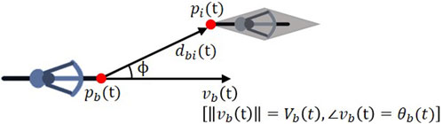
FIGURE 2. Graphical representation of the vectors and angles included in the models.

In response to the presence of the interacting road user $i$ in Figure 2, the depicted cyclist $b$ will reduce their speed ($∆V_b\left(t\right)<0$) and will change direction away from the interacting road user in the clockwise direction ($∆{\theta }_b\left(t\right)<0$).

In addition to separating the model into the norm and angle representation of the velocity vector, the original NOMAD model is adapted in two important ways. First, the reaction to a traffic signal is included directly in the change in speed model. This is done by mimicking the reaction of a cyclist to a large interacting road user that cannot be passed. The outline of the signalized intersection is denoted by a polygon that connects the stop lines of all the approaches. The nearest point on the stop line polygon to $p_b\left(t\right)$ is selected as $p_s\left(t\right)$. The distance vector $d_s\left(t\right)=p_s\left(t\right)-p_b\left(t\right)$ and norm $D_s\left(t\right)=‖d_s\left(t\right)‖$ are analogous to the variables defined for interacting with road users. This is only done for the change in speed model because cyclists cannot maneuver around traffic signals.

Second, instead of using a constant bicycle-specific parameter to control the interaction response $A_{vb}$, a variable is defined based on the current speed $V_b\left(t\right)$, the desired speed $V_b^0$ and the speed relaxation parameter $T_{vb}$ that ensures simulated cyclists are able to stop in any simulation second. If the current speed $V_b\left(t\right)$ is large, the interaction response $A_{vb}$ also increases in magnitude to allow for a stronger deceleration response to avoid collisions in all possible situations. In addition, this conversion reduces the number of parameters in the model by one, enabling a more stable prediction of the remaining model parameters.

$A_{vb}=\frac{V_b^0+\left(T_{vb}-1\right)V_b\left(t\right)}{T_{vb}}(9)$

The equation describing the change in direction $∆{\theta }_b\left(t\right)$ (Eq. 7) is formulated similarly; ${\theta }_b\left(t\right)$ is the direction of travel of cyclist $b$ at time t, and $T_{\theta b}$, $A_{\theta b,}$ and $R_{\theta b}$ are constant cyclist specific parameters controlling the change of direction specifically. $U_{bi}\left(t\right)$ is introduced to specify the position of the interacting road user concerning the desired path of travel and enables cyclist $b$ to move to the left in response to a road user on the right and vice versa. $U_{bi}\left(t\right)$ can take a value of either $-1$ or $1$ depending on the side of the interacting road user relative to the velocity of bicycle $b$. The main difference between Eq. 6 and Eq. 7 is that ${\theta }_b^0\left(t\right)$ is not a static parameter, as $V_b^0$ is in Eq. 6, but rather changes to guide cyclist $b$ along his or her desired pathway across the intersection. The desired change in direction based on the desired position of cyclists $b$ at time $t$ is shown in Figure 3.

FIGURE 3

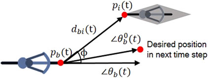
FIGURE 3. Graphical representation of the definition of desired change of direction.

The summation across all interacting road users in the set $IRU$ is restricted to the change in angle equation (Eq. 7). This reflects the interacting behavior of road users. It is presumed that a cyclist adapts their speed based only on the most critical of interacting road users. For example, when riding in a single-file platoon of cyclists, a cyclist does not ride slower if there are many cyclists ahead in the platoon than he would if there were only one cyclist ahead. The speed is determined to prevent a collision with the most critical interacting road user. In contrast, the direction is adapted as a response to many other road users within a given area. This enables the cyclist to maneuver through a group of cyclists. Furthermore, it is presumed that cyclists do not react to road users positioned behind themselves, and to this effect the indicator function $1_{\varphi <\pi /2}$ is deployed in all models includes the basic model. This presumption was confirmed through initial evaluations of models including interacting with road users in all directions.

2.2 Anisotropic model

The first variation of the basic model examined here is an adaptation of the anisotropic NOMAD model, which takes into account the position of the interacting road user $i$ with respect to the direction of travel of cyclist $b$. Using this approach, road users directly in the line of travel of cyclist $b$ have the largest impact on the change in speed $∆V_b\left(t\right)$ and direction $∆{\theta }_b\left(t\right)$. This extension reflects the behavior hypothesis that cyclists, like pedestrians, react to those in their field of vision (not behind them) and those who are “in the way” of planned movement. The formulation of the anisotropic model is given in Eqs 10, 11:

$∆V_b\left(t\right)=\frac{V_b^0-V_b\left(t\right)}{T_{vb}}-A_{vb}{e}^{\frac{-{\mathit{min}}_i\left\{D_s,D_{bi}^{\ast }\left(t\right)\right\}}{R_{vb}}}{1}_{\varphi <\frac{\pi }{2}}(10)$

$∆{\theta }_b\left(t\right)=\frac{{\theta }_b^0\left(t\right)-{\theta }_b\left(t\right)}{T_{\theta b}}-A_{\theta b}{\displaystyle \sum _{i\in IRU}}{U}_{bi}\left(t\right)e^{\frac{-D_{bi}^{\ast }\left(t\right)}{R_{\theta b}}}{1}_{\varphi <\frac{\pi }{2}}(11)$

where:

$D_{bi}^{*}\left(t\right)=\frac{d_{bi}\left(t\right)\bullet v_b\left(t\right)}{V_b\left(t\right)}+{\eta }_b\frac{d_{bi}\left(t\right)\bullet w_b\left(t\right)}{V_b\left(t\right)}(12)$

Here, the distance between cyclist $b$ and road user $i$ is divided into two components, one parallel and the other perpendicular to the direction of travel of cyclist $b$. The vector $w_b\left(t\right)$ is perpendicular to $v_b\left(t\right)$ with the same scalar quantity and is oriented in the direction of road user $i$. The bicycle-specific parameter ${\eta }_b$ describes the weighting of the distance of two components relative to one another (${\eta }_b>1$). Two different values of ${\eta }_b$ are solved for in the model, one for the $∆V_b\left(t\right)$ component (${\eta }_{vb}$) and one for the $∆{\theta }_b\left(t\right)$ component (${\eta }_{\theta b}$).

2.3 Velocity anisotropic model

A final extension is proposed here to include the direction of travel of the interacting road user in the change of speed and change of direction model. The behavior hypothesis behind this extension is that cyclists have a less pronounced response to interacting road users moving with a similar velocity. For example, a cyclist moving in a platoon of other cyclists will only make minimal adjustments to his or her speed in response to a leading cyclist moving in the same direction with a similar speed, even though this leading cyclist may be very close in terms of distance. In contrast, the response to another road user moving towards cyclist $b$ will be much larger, even if this road user is further away. To account for this aspect of behavior, the effective distance $D_{bi}^{**}\left(t\right)$ is increased or decreased depending on the velocity vector of the interacting road user in relation to that of cyclist $b$.

$∆V_b\left(t\right)=\frac{V_b^0-V_b\left(t\right)}{T_{vb}}-A_{vb}{e}^{\frac{-{\mathit{min}}_i\left\{D_s,D_{bi}^{**}\left(t\right)\right\}}{R_{vb}}}{1}_{\varphi <\frac{\pi }{2}}(13)$

$∆{\theta }_b\left(t\right)=\frac{{\theta }_b^0\left(t\right)-{\theta }_b\left(t\right)}{T_{\theta b}}-A_{\theta b}{\displaystyle \sum _{i\in IRU}}{U}_{bi}\left(t\right)e^{\frac{-D_{bi}^{**}\left(t\right)}{R_{\theta b}}}{1}_{\varphi <\frac{\pi }{2}}(14)$

where:

$D_{bi}^{**}\left(t\right)=\frac{d_{bi}\left(t\right)\bullet v_b\left(t\right)}{V_b\left(t\right)}+{\eta }_b\frac{d_{bi}\left(t\right)\bullet w_b\left(t\right)}{V_b\left(t\right)}+{\gamma }_b\frac{v_i\left(t\right)\bullet v_b\left(t\right)}{V_i\left(t\right)V_b\left(t\right)}(15)$

The parameter ${\gamma }_b$ reflects the bicycle-specific adjustment of the effective distance depending on the similarity between the velocity of the interacting road user $i$ and that of bicycle $b$. The cosine of the angle between $v_i$ and $v_b$ ($\frac{v_i\left(t\right)\bullet v_b\left(t\right)}{V_i\left(t\right)V_b\left(t\right)}$) ranges between $-1$ and $1$ and as such the parameter ${\gamma }_b$ represents the adjustment of the effective distance in meters. Two different values of ${\gamma }_b$ are solved in the model, one for the $∆V_b\left(t\right)$ component (${\gamma }_{vb}$) and one for the $∆{\theta }_b\left(t\right)$ component (${\gamma }_{\theta b}$).

2.4 Parameter estimation

For each of the proposed models, there are several cyclist-specific parameters to be calibrated using observed trajectory data (Table 1). Trajectories from cyclists were extracted from video data collected at four signalized intersections in Munich, Germany (Twaddle et al., 2014b). Videos were recorded during the spring and summer months of 2013 and 2014 for between two and 4 days per intersection. The observation period began at approximately 7:00 a.m. and ended at about 7:00 p.m. The open-source software Traffic Intelligence (Saunier, 2016) was used for automated extraction of trajectories of a sub-set of videos and the resulting trajectory database was manually controlled and corrected. A total of 634 high-quality trajectories were used for model calibration and validation (k-fold cross-validation).

TABLE 1

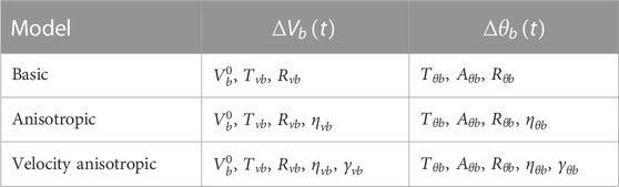
TABLE 1. Model parameters to be calibrated.

The observed values for $p_b\left(t\right)$, $v_b\left(t\right)$ and $p_i\left(t\right)$, $v_i\left(t\right)$ for all interacting road users in the set $IRU$ are extracted from the trajectory data for each time step $t$ for each cyclist $b$.

Each trajectory has the form $S_b=\left[\begin{array}{cc}{\left(x_b,y_b\right)}_{t=0}& {\left(x_b,y_b\right)}_{t=1}\cdots {\left(x_b,y_b\right)}_{t=T_b}\end{array}\right]$, where ${\left(x_b,y_b\right)}_t$ is the position coordinate of cyclist $b$ at time $t$ and $T_b$ is the duration of the trajectory. Here, the position observations are aggregated such that the frequency of 25 observations per second is reduced to 8.33 (25/3) observations per second. The noise in the position data was partially resolved through this aggregation. The aggregated position points are smoothed using the Savitzky–Golay filter (Savitzky and Golay, 1964). The change in speed and change in direction observations are derived from the smoothed and aggregated trajectories.

The remaining vectors $d_{bi}\left(t\right)$ and $w_b\left(t\right)$, angle $\varphi$ and the value $U_{bi}\left(t\right)$ are calculated from the $p_b\left(t\right)$, $v_b\left(t\right)$, $p_i\left(t\right)$ and $v_i\left(t\right)$ observations. In each time step, a presumed desired direction ${\theta }_b^0\left(t\right)$ is inferred using the representative trajectory for the cluster to which cyclist $b$ is found to belong. The representative trajectory is assumed to embody the desired position points of each cyclist along their trajectory. Without this assumed desired trajectory, it is not possible to generate a ${\theta }_b^0\left(t\right)$ in each time step. The desired direction in time step $t$ is found by locating the point on the representative trajectory nearest to $p_b\left(t\right)$ (point $l_1$ in Figure 4). A second point is specified at a distance $\overline{V^0}$ further along the representative trajectory (point $l_1+\overline{V^0}$ in Figure 4). The first point is necessary to act as a starting point for measuring the distance $\overline{V^0}$ along the representative trajectory. A vector is drawn between $p_b\left(t\right)$ and this second point, the angle of which is taken to be ${\theta }_b^0\left(t\right)$. A graphical representation of this approach is shown in Figure 4.

FIGURE 4

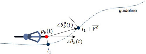
FIGURE 4. Graphical representation of the approach for finding ${\mathit{\theta }}_{\mathit{b}}^{\mathbf{0}}\left(\mathit{t}\right)$.

The model parameters are calibrated to fit the observed behavior using Maximum Likelihood Estimation (MLE). This method provides a means for deriving the values of a set of parameters $\left.\beta ={\left\{\beta \right.}_0,{\beta }_1,{\beta }_2,\dots {\beta }_m\right\}$ in a model to best fit a sample of data. This is achieved by expressing the likelihood as a joint probability mass function of the sample of observations as shown in Eq. 16 and Eq. 17. The likelihood $L\left(\beta \right)$ is a function of the parameter set $\beta$ and is maximized to find the optimal set of parameters.

$L\left(\beta \right)=P\left(X_1=x_1,X_2=x_2,\dots ,X_n=x_n\right)(16)$

$L\left(\beta \right)=f\left(x_1;\beta \right)\bullet f\left(x_2;\beta \right)\bullet \bullet \bullet f\left(x_n;\beta \right)={\displaystyle \prod _{i=1}^n}f\left(x_i;\beta \right)(17)$

Assuming that the observations are normally distributed, the probability mass function can be expressed using Eq. 18 and the joint probability mass function or likelihood of $\beta$ is given by Eq. 19

$f\left(x_i;\beta \right)=\frac{1}{\sqrt{2\pi {\sigma }^2}}{e}^{\left(-\frac{{\left(x_i^{pred}-x_i^{obs}\right)}^2}{2{\sigma }^2}\right)}(18)$

$L\left(\beta \right)={\displaystyle \prod _{i=1}^n}f\left(x_i;\beta \right)={\displaystyle \prod _{i=1}^n}\frac{1}{\sqrt{2\pi {\sigma }^2}}{e}^{\left(-\frac{{\left(x_i^{pred}-x_i^{obs}\right)}^2}{2{\sigma }^2}\right)}(19)$

The log of the likelihood $\mathcal{L}\left(\beta \right)$ is typically maximized:

$\mathcal{L}\left(\beta \right)=-\frac{n}{2}\ln \left(2\pi {\sigma }^2\right)-\frac{1}{2{\sigma }^2}{\displaystyle \sum _{i=1}^n}{\left(x_i^{pred}-x_i^{obs}\right)}^2(20)$

The standard deviation ${\sigma }^2$ must be determined in order to numerically solve for the best fitting parameter set $\beta$. The maximum likelihood estimator of the variance is given in Eq. 21.

${\widehat{\sigma }}^2=\frac{1}{n}{\displaystyle \sum _{i=1}^n}{\left(x_i^{pred}-x_i^{obs}\right)}^2(21)$

The log likelihood function given ${\widehat{\sigma }}^2$ is expressed in Eq. 22. Using this function, the parameter set $\widehat{\beta }$ can be solved for using numerical optimization.

$\mathcal{L}\left(\beta ;{\widehat{\sigma }}^2\right)=-\frac{n}{2}\ln \left(\frac{2\pi }{n}{\displaystyle \sum _{i=1}^n}{\left(x_i^{pred}-x_i^{obs}\right)}^2\right)-\frac{n}{2}(22)$

$\widehat{\beta }=\arg \max \mathcal{L}\left(\beta ;{\widehat{\sigma }}^2\right)(23)$

Trajectory data from each of the observed cyclists at three of the four research intersections were used to estimate parameters. The parameter set for each cyclist is denoted as ${\beta }_b$ and includes the parameters shown in Table 1. The model parameters are calibrated for each observed cyclist using the following equations:

$\mathcal{L}\left({\beta }_b;{\widehat{\sigma }}_b^2\right)=-\frac{n}{2}\ln \left(\frac{2\pi }{n}{\displaystyle \sum _{i=1}^n}{\left(a_i^{pred}-a_i^{obs}\right)}^2\right)-\frac{n}{2}(24)$

${\widehat{\beta }}_b=\arg \max \mathcal{L}\left({\beta }_b;{\widehat{\sigma }}_b^2\right)(25)$

where $n$ is the number of observation points along the aggregated trajectory. To ensure that $n$ is large enough to find stable estimates of ${\widehat{\beta }}_b$, samples with fewer than 50 observations are filtered out from the dataset. This reflects the recommendation by Long (Long, 1997) to include at least 10 observations per parameter. The majority of the trajectories include between 100 and 250 observation points.

The maximum log likelihood is numerically solved using the SciPy Python implementation (The Scipy community, 2016) of the Constrained Optimization BY Linear Approximation (COBYLA) algorithm proposed by Powell (Powell, 1994). Using this method, it is possible to set constraints that prevent the algorithm from locating an illogical, but mathematically optimal, minimum (e.g., extremely large desired velocity $V_b^0$ and relaxation time $T_b$ pairs). Initial estimates of the parameters are supplied to the algorithm.

2.5 Model evaluation

The models are evaluated using K-fold cross-validation. Using this method, the sample of observations ($n$ per cyclist) is randomly divided into $K$ mutually exclusive sub-samples of approximately equal size. The calibration of the parameter set is repeated $K$ times (or folds). In each fold, a sub-sample is held back from the model calibration and the parameter set ${\widehat{\beta }}_{bsub-sample}$ are estimated using the remainder of the dataset. The calibrated model is then validated using the held back sub-sample. The model predictions are made by taking the observed position and velocity of the road users at each time step, extracting or calculating the model vectors and scalars, and computing the predicted $∆V_b\left(t\right)$ and $∆{\theta }_b\left(t\right)$. These predictions are compared to the actual change in speed and angle observed at that time step. This type of validation reduces potential influence from the random splitting of the data because each of the observations is used exactly once for validation.

In order to assess the predictive power of the models, the performance is compared to the constant velocity model in which acceleration equals zero in each time step (null case). Although this model is not capable of simulating traffic, it provides a useful method to determine if the predictions made in each time step are significantly better than a prediction of $0$. Two measures are used to compare the developed models with this base model. The average improvement in log likelihood and the log likelihood ratio test. The average improvement in log likelihood, which indicates the overall improvement in model performance, is given by Eq. 26:

$I=\frac{{\displaystyle \sum _{b\in B}}\mathcal{L}\left({\beta }_b;{\widehat{\sigma }}^2\right)-{\displaystyle \sum _{b\in B}}{\mathcal{L}}_{bnull}}{‖{\displaystyle \sum _{b\in B}}{\mathcal{L}}_{bnull}‖}(26)$

Where $B$ is the set of observed cyclists and ${\mathcal{L}}_{bnull}$ is the log likelihood of the constant velocity model. The log likelihood ratio test is a statistic that enables the comparison between models of differing complexities. Because model estimations inherently improve with each additional parameter, the magnitude of this improvement with respect to the increase in degrees of freedom must be examined to determine if a complex model is better. The test statistic for the log likelihood ratio test is given by:

$D=2\left(\mathcal{L}\left({\beta }_b;{\widehat{\sigma }}_b^2\right)-{\mathcal{L}}_{bnull}\right)(27)$

$D$ is compared with the critical value ${\chi }^2$ from the chi-squared distribution with degrees of freedom $df={df}_{alternative}-{df}_{null}$. The degrees of freedom ${df}_{alternative}$ is the number of parameters for each model shown in Table 1. Models are accepted as significantly better if $p<0.1$. The percentage of models (one model per observed cyclist) that pass this test is used as an assessment measure for the overall model performance. The calibration and validation algorithm implemented here is shown in pseudo code below. All three model variations are tested using this approach.

The models are tested using different delay times that represent the reaction times of the observed cyclists. It is presumed that, like motorists, cyclists do not respond immediately to stimuli in the road environment. Instead, a certain amount of time is required to collect sensory information, process this data, decide upon an appropriate response, and carry out this response. Mean reaction times for car drivers have been estimated to lie between 0.7–1.5 s (Green, 2007). To reflect this reaction time, the acceleration observations are collected at $t+\tau$ for observations from time step $t$. Values of $\tau$ ranging between 0.0 s and 1.5 s are tested and the model quality is assessed using $I$ (Eq. 26) and the percentage of models that pass the log likelihood ratio test (Eq. 27).

3 Results

The parameter distributions for the calibrated change in speed model are shown and are briefly discussed in the first section followed by the results for the calibrated change in angle model. The best-suited reaction time $\tau$ is located by examining the overall percent increase in the log likelihood $I$ and the percent of calibrated models that pass the log likelihood ratio test for each reaction time $\tau$ between 0 s and 1.5 s at an interval of 0.12 s. The lowest reaction time $\tau$ leading to markedly improved model performance is selected and the calibrated model parameters for this reaction time are presented.

3.1 Change in speed

The evaluation measures for the varying reaction time $\tau$ values are shown in Figure 5. A reaction time $\tau$ of 1.2 s leads to the best prediction of change in speed values. This lies within the range suggested by Green (Green, 2007) for car drivers but is considerably larger than the 0.28 s found by Hoogendoorn and Daamen (Hoogendoorn and Daamen, 2007) for pedestrians.

FIGURE 5

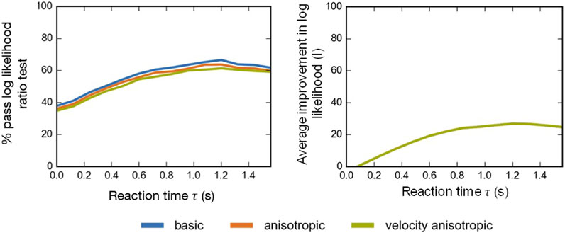
FIGURE 5. Evaluation of the calibrated change in speed models for varying reaction times $\mathit{\tau }$.

Based on a qualitative assessment of the distributions shown in Figure 6, the calibrated model parameters are deemed to be roughly represented by the normal distribution, although the lognormal distribution may be more appropriate for the parameters $T_{vb}$ and ${\gamma }_{vb}$. Nevertheless, all parameters here were defined using the mean and standard deviation, as listed in Tables 2–4. The magnitudes of these distribution parameters fall within an expected range of values and the consistency between parameters occurring in multiple models, $V_b^0$, $R_{vb}$, $T_{vb}$ and ${\eta }_{vb}$, indicates the stability of the parameter outputs from the maximum likelihood estimation. The resulting parameter distributions of the basic and anisotropic models closely resemble those shown for the velocity anisotropic model shown in Figure 6.

FIGURE 6

FIGURE 6. Distributions of calibrated model parameters for the ${\Delta \mathit{V}}_{\mathit{b}}\left(\mathit{t}+\mathit{\tau }\right)$ velocity anisotropic model.

TABLE 2

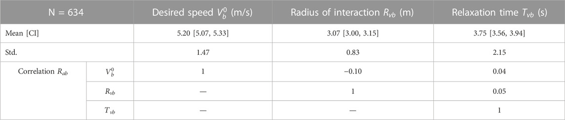
TABLE 2. Calibration results for ${\mathbf{\Delta }\mathit{V}}_{\mathit{b}}\left(\mathit{t}+\mathit{\tau }\right)$ basic model (reaction time: $\mathit{\tau }=\mathbf{1.2}\mathit{s}$).

TABLE 3

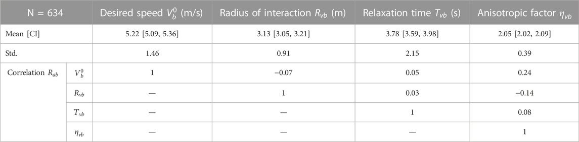
TABLE 3. Calibration results for the ${\mathbf{\Delta }\mathit{V}}_{\mathit{b}}\left(\mathit{t}+\mathit{\tau }\right)$ anisotropic model (reaction time: $\mathit{\tau }=\mathbf{1.2}\mathit{s}$).

TABLE 4

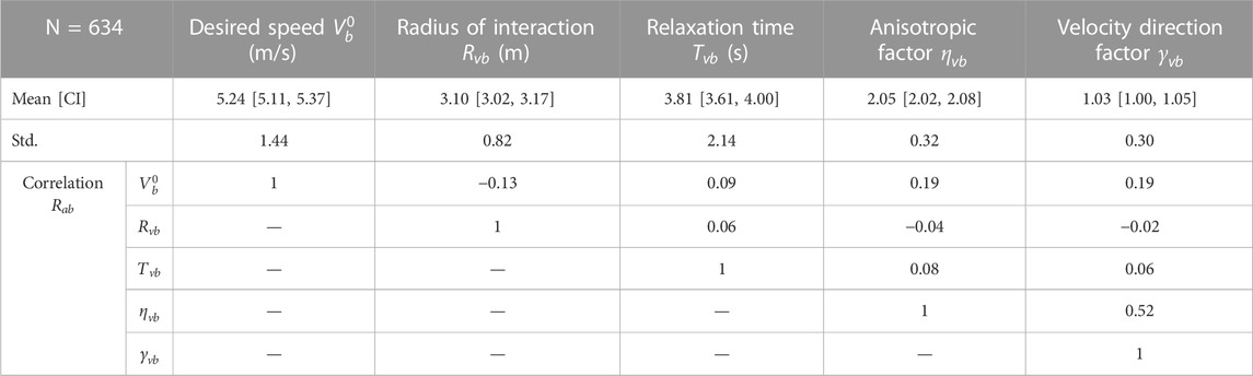
TABLE 4. Calibration results for ${\mathbf{\Delta }\mathit{V}}_{\mathit{b}}\left(\mathit{t}+\mathit{\tau }\right)$ velocity anisotropic model (reaction time: $\mathit{\tau }=\mathbf{1.2}\mathit{s}$).

The correlations between the model parameters are also important to consider and include in the subsequent traffic simulation to avoid incompatible parameter combinations. The Pearson correlation coefficient between the parameters is calculated using the formula below:

$R_{ab}=\frac{n\sum ab-\sum a\sum b}{\sqrt{\left(n\sum a^2-{\left(\sum a\right)}^2\right)\left(n\sum b^2-{\left(\sum b\right)}^2\right)}}(28)$

where $n$ is the number of observations, and $a$ and $b$ are variables for which the correlation is to be determined. The resulting correlation ranges between −1 and 1, with 0 indicating no correlation between parameters.

In the meta-analysis of 28 studies that measure the speed of cyclists (Twaddle, 2017), a median value of 4.6 m/s (16.5 km/h) was found. The higher value of 5.2 m/s (18.7 km/h) found here is logical because this value represents the desired speed of a population of cyclists rather than the realized or observed speeds. Realized speeds are per definition lower as the cyclist must slow to avoid other road users and obstacles and react to the signal control.

The relaxation time is a proxy measure for the maximum acceleration. If the mean relaxation time of 3.8 s is combined with the mean desired speed, a maximum acceleration of 1.4 m/s² emerges. The acceleration rate is slightly higher than those found in the literature (Parkin and Rotheram, 2010) but falls within a reasonable range. This is also expected as it is based on desired speed and not observed speed. A radius of interaction of 3.1 m appears reasonable but cannot be assessed in comparison to the findings of other research because none were found. The mean and standard variations of the parameters ${\eta }_{vb}$ and ${\gamma }_{vb}$ are realistic and signify an average cyclist that weights interacting road users directly in the path of travel with roughly twice the importance of those directly to the side. Roughly 1 m is subtracted from the effective distance $D_{bi}^{**}$ if the interacting road user is traveling with the same velocity as cyclist $b$ and added if the velocity is opposite.

The correlations between the calibrated model parameters are quite small. The most noteworthy correlations are the positive correlation between the desired speed and both the anisotropic and velocity direction factor, the negative correlation between the desired speed and the radius of interaction, and the correlation between the anisotropic factor and the velocity direction factor. Together these correlations indicate that cyclists who aim to travel with a higher speed have a slightly smaller interaction zone and are more focused on interacting with road users directly in their planned pathway and those with an opposing velocity vector. This may point to a group of cyclists who are faster, more confident, and who are more likely to accept risk.

3.2 Change in angle

The equation for predicting the change in angle proved to be much more difficult to calibrate than that for the change in speed. This is due to the inherent difficulty in isolating the desired change in angle. Here, the representative trajectory of a cluster of cyclists is used to approximate the desired direction of travel of a cyclist at each position while crossing the intersection. The desired direction in each time step ${\theta }_b^0\left(t\right)$ is therefore based on the representative trajectory for the cluster to which cyclist $b$ is assigned. It is very likely, however, that the actual desired direction ${\theta }_b^0\left(t\right)$ varied (slightly or greatly) from the approximated value. Another difficulty arises due to noise in the trajectory data. Although the high angle of the video camera to the intersections and smoothing the trajectory data reduced the amount of noise, small variations in the tracked centroid likely have a small impact on the quality of the model calibration. Nevertheless, the calibrated models proved to be a significant improvement over the constant velocity model for more than half of the observed cyclists. Considering that ${\Delta \theta }_b\left(t\right)$ lies very close to zero in each time step of 0.12 s and the lack of concrete data describing the desired direction, the results presented below are exceptional.

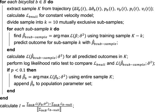
The evaluation parameters for the calibrated models, the average improvement in log likelihood $I$ (Eq. 26) and percent passing the log likelihood ratio test, for reaction times $\tau$ ranging between 0 s and 1.5 s with an interval of 0.12 s are shown in Figure 7.

FIGURE 7

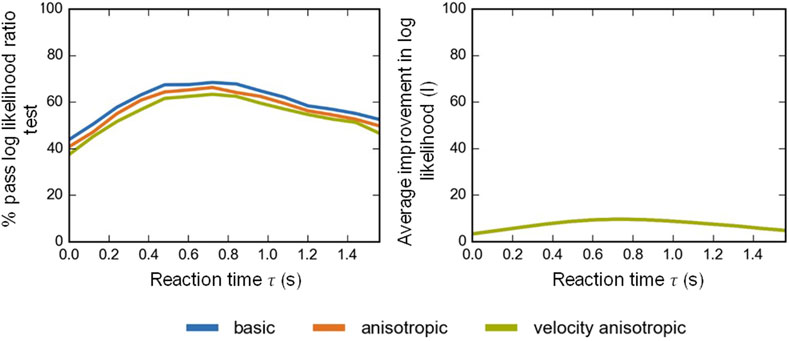
FIGURE 7. Evaluation of the calibrated change in angle models for varying reaction times $\mathit{\tau }$.

The optimal reaction time $\tau$ lies between 0.4 s and 0.8 s, which is lower than the range identified for the ${\Delta V}_b\left(t\right)$ portion of the model (∼1.2 s). Although the perception and processing components of the reaction time are the same for both actions, the different levels of complexity associated with the tasks may account for the difference in overall reaction time. This may indicate that cyclists can react faster to stimuli by adjusting their direction of travel rather than their speed. A reaction time of $\tau =0.6s$ for change in direction is selected and the calibrated model parameters from this reaction time are presented and evaluated.

The calibrated model parameter distributions are shown in Figure 8. Based on a qualitative assessment of the distributions, the hypothesis of normal distribution is rejected for the interaction factor $A_{\theta b}$, the radius of interaction $R_{\theta b}$, the anisotropic factor ${\eta }_{\theta b}$ and the velocity direction factor ${\gamma }_{\theta b}$. All of these factors show a very small deviation around a centric value. For this reason, the median value of each calibrated parameter is selected as a constant for the entire population of cyclists. This simplifies the models for the simulation. The means, confidence intervals, and standard deviations are nevertheless reported in Tables 5–7 if the reader is interested. The relaxation time $T_{\theta b}$ is deemed to be normally distributed and as such a bicycle specific parameter is used.

FIGURE 8

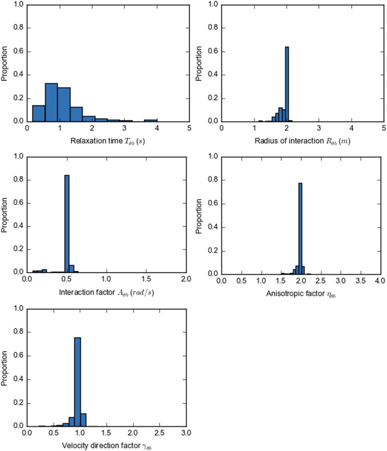
FIGURE 8. Distributions of calibrated model parameters for the ${\Delta \mathit{\theta }}_{\mathit{b}}\left(\mathit{t}+\mathit{\tau }\right)$ velocity anisotropic model.

TABLE 5

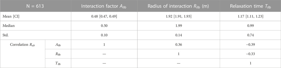
TABLE 5. Calibration results for the ${\mathbf{\Delta }\mathit{\theta }}_{\mathit{b}}\left(\mathit{t}+\mathit{\tau }\right)$ basic model (reaction time: $\mathit{\tau }=\mathbf{0.6}\mathit{s}$).

TABLE 6

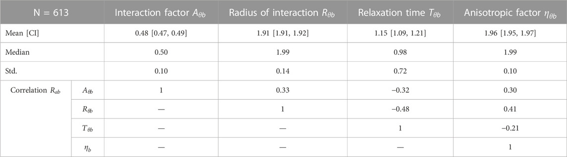
TABLE 6. Calibration results for the ${\mathbf{\Delta }\mathit{\theta }}_{\mathit{b}}\left(\mathit{t}+\mathit{\tau }\right)$ anisotropic model (reaction time: $\mathit{\tau }=\mathbf{0.6}\mathit{s}$).

TABLE 7

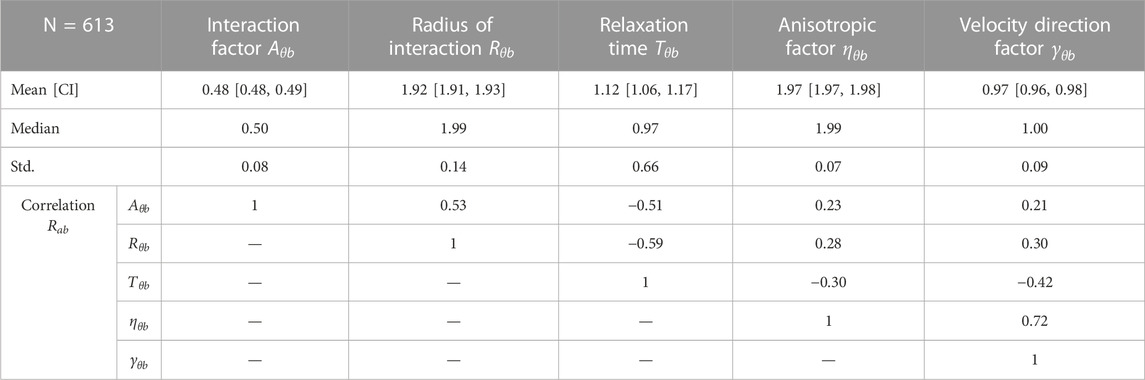
TABLE 7. Calibration results for the ${\mathbf{\Delta }\mathit{\theta }}_{\mathit{b}}\left(\mathit{t}+\mathit{\tau }\right)$ velocity anisotropic model (reaction time: $\mathit{\tau }=\mathbf{0.6}\mathit{s}$).

The calibrated parameters have the expected magnitude and sign. However, it is difficult to compare the results to the findings of other studies because no studies were identified that examined the response of other road users regarding the change in direction (without a change in speed). The mean of the interaction factor $\overline{A_{\theta b}}=0.48rad/s$ (28°/s) signifies the maximum response to an interacting road user. The calibrated relaxation time for the change in direction models is considerably lower than that in the change in speed portion of the model. This makes logical sense as changes in direction, which tend to be quite small, are realized without significant delay. This value, however, is highly dependent on the desired direction ${\theta }_b^0\left(t\right)$, which as stated before, is difficult to isolate based on observed trajectory data. The anisotropic factor ${\eta }_{\theta b}$ and the velocity direction factor ${\gamma }_{\theta b}$ agree very strongly with the calibrated values found for the change in speed portion of the model and appear to be realistic.

The Spearman correlation coefficient $R_{ab}$ between the parameters (assuming normal distribution) are shown in Tables 5–7 but are not investigated further as the cyclist specific parameters $A_{\theta b}$, $R_{\theta b}$, ${\eta }_{\theta b}$, ${\gamma }_{\theta b}$ were found to be adequately represented by the population parameters $A_{\theta }$, $R_{\theta }$, ${\eta }_{\theta }$, ${\gamma }_{\theta }$. These population parameters are set as the median value for the observation.

4 Discussion

This paper presents a modeling approach for the movement and interactions of cyclists and other non-lane-based road users. The model belongs to the family of social force models, making it possible to capture the flexibility and fluidity of the behavior exhibited by these road users. However, by integrating guidelines, or desire lines, that are “followed” by the road user and can defined using the center lines of (sub-)lanes in microscopic traffic simulations, it is possible to easily integrate this model in car-based simulations and maintain the largely longitudinal directions of travel. The evaluation of the model indicates a significant improvement in comparison to a constant velocity model. The estimated parameters are found to be realistic and the reaction times for the change in speed and change in direction models are feasible. The lower reaction time estimated for the change of direction model in comparison to the change in speed model suggests that cyclists more readily swerve to avoid conflict than decelerate. The models have only been validated using the Munich trajectory dataset. Using another trajectory data set for validation would be a useful future step.

In comparison to motor vehicle or even pedestrian traffic, significantly less research has focused on modeling and simulating the movement and interactions of non-lane-based road users. One reason for this has been the overall lack of the type of data needed to adequately formulate and calibrate microscopic behavior models as simulations that include these road users. Count data that is typically used to calibrate and validate car simulations is insufficient for non-lane-based traffic because no information about the lateral position of the road users is included. Developments in technologies that make it possible to collect large samples of accurate trajectory data, including automated video processing and LIDAR data processing, will make it possible to carry out model calibration and validation at the trajectory level.

Not only observational data but experimental data are needed to gain insight into the behaviors exhibited by non-lane-based road users. In this paper, the desired direction of travel is estimated using the centroid of a cluster of trajectories, which is a weak hypothesis, as we cannot observe the intended path of travel. An example of an experiment that could be carried out is setting a line to be followed by a cyclist and observing deviations due to interactions with other road users or the environment.

Another issue that affects the evaluation and comparison of behavior models for non-lane-based road users is the lack of previous work defining validation parameters. For example, traffic density for non-lane-based traffic cannot be measured in vehicles/distance (veh/km) but instead has to be measured in vehicles/area (bicycle/m²). Furthermore, it cannot be assumed that cyclists or users of micro-mobility always use the road infrastructure as intended. Switching between cycling infrastructure (if available), the roadways and the sidewalk, riding against the given direction of travel, and crossing intersections using unexpected pathways are examples of the flexible behavior exhibited by cyclists and micro-mobility users. In Twaddle (Twaddle, 2017), heat maps were used to include the spatial distribution of cyclists over entire intersections to assess the validity of the modeling approach. However, much more work is necessary to systematically define useful parameters for the evaluation of microscopic traffic simulation of non-lane-based traffic in the same way that has been done for lane-based traffic (see, for example, (Forschungsgesellschaft für Straßen-und Verkehrswesen, 2006)).

Once sufficient data is available, a foundation of knowledge about the movement and interactions of cyclists is established, and information about users of micro-mobility modes and other non-lane-based traffic is gathered, it will be possible to develop and compare behavior models for microscopic traffic simulation. It will be possible to determine whether (sub-)lane based models, social force type models, hybrid models, such as the model presented here, or other types of models best recreate the movement and interactions of cyclists, users of micro-mobility modes, and other non-lane-based road users.

Data availability statement

The datasets presented in this article are not readily available. The data are stored at the Chair of Traffic Engineering and Control at the Technical University of Munich (Germany) and can be requested by contacting this department. Requests to access the datasets should be directed to info.vtk@ed.tum.de.

Author contributions

HK is the sole author of this paper. She conceived, formulated, and implemented the operational behavior model, collected and prepared the trajectory data used for calibrating the model, carried out the model evaluation, and wrote the paper.

Funding

This research was partially supported by the Federal Ministry of Economic Affairs and Climate Action based on a decision by the German Bundestag. Research was carried out within the framework of the project UR:BAN (Urban Space: User oriented assistance systems and network management).

Conflict of interest

The author declares that the research was conducted in the absence of any commercial or financial relationships that could be construed as a potential conflict of interest.

Publisher’s note

All claims expressed in this article are solely those of the authors and do not necessarily represent those of their affiliated organizations, or those of the publisher, the editors and the reviewers. Any product that may be evaluated in this article, or claim that may be made by its manufacturer, is not guaranteed or endorsed by the publisher.

References

Falkenberg, G., Blase, A., Bonfranchi, T., Cosse, L., Draeger, W., Vortisch, P., et al. (2003). Bemessung von Radverkehrsanlagen unter verkehrstechnischen Gesichtspunkten. Berichte Bundesanst. fuer Strassenwes. Unterr Verkehrstechnik. 103.

Google Scholar

Fellendorf, M., and Vortisch, P. (2010). “Microscopic traffic flow simulator VISSIM,” in Fundamentals of traffic simulation (Cham: Springer), 63–93.

CrossRef Full Text | Google Scholar

Forschungsgesellschaft für Straßen- und Verkehrswesen (2006). Hinweise zur mikroskopischen Verkehrsflusssimulation: Grundlagen und Anwendung Vol. 388. Wesselinger: FGSV Verlag.

Google Scholar

Green, P. (2007). Why driving performance measures are sometimes not accurate (and methods to check accuracy). Proc. Fourth Int. Driv. Symp. Hu Man. Factors Driv. Assess. Train. Veh. Des., 394–400. doi:10.17077/drivingassessment.1267

CrossRef Full Text | Google Scholar

Helbing, D., and Molnar, P. (1995). Social force model for pedestrian dynamics. Phys. Rev. E 51 (5), 4282–4286. doi:10.1103/physreve.51.4282

PubMed Abstract | CrossRef Full Text | Google Scholar

Hoogendoorn, S. P., and Daamen, W. (2007). “Microscopic calibration and validation of pedestrian models: cross-comparison of models using experimental data,” in Traffic and granular Flow’05 (Cham: Springer), 329–340.

Google Scholar

Hoogendoorn, S. P. (2001). Normative pedestrian flow behavior theory and applications. Delft, Netherlands: Delft University of Technology, Faculty Civil Engineering and Geosciences.

Google Scholar

Khan, S., and Raksuntorn, W. (2001). Characteristics of passing and meeting maneuvers on exclusive bicycle paths. Transp. Res. Rec. J. Transp. Res. Board 1776 (1), 220–228. doi:10.3141/1776-28

CrossRef Full Text | Google Scholar

Krajzewicz, D., Erdmann, J., Härri, J., and Spyropoulos, T. (2014). “Including pedestrian and bicycle traffic in the traffic simulation SUMO,” in 10th ITS European Congress Helsinki, Finland, 16–19 June, 2014, 1–10.

Google Scholar

Li, M., Shi, F., and Chen, D. (2011). “Analyze bicycle-car mixed flow by social force model for collision risk evaluation,” in 3rd Int Conf Road Saf Simul., Indianapolis Indiana, United States, September 14–16, 2011. 1–22.

Google Scholar

Li, Y., Ni, Y., and Sun, J. (2021). A modified social force model for high-density through bicycle flow at mixed-traffic intersections. Simul. Model Pract. Theory 108, 102265. doi:10.1016/j.simpat.2020.102265

CrossRef Full Text | Google Scholar

Liang, X., Mao, B., and Xu, Q. (2012). Psychological-physical force model for bicycle dynamics. J. Transp. Syst. Eng. Inf. Technol. 12 (2), 91–97. doi:10.1016/s1570-6672(11)60197-9

CrossRef Full Text | Google Scholar

Lind, A., Honey-Rosés, J., and Corbera, E. (2021). Rule compliance and desire lines in Barcelona’s cycling network. Transp. Lett. 13 (10), 728–737. doi:10.1080/19427867.2020.1803542

CrossRef Full Text | Google Scholar

Long, J. S. (1997). “Regression models for categorical and limited dependent variables,” in Vol. 7, advanced quantitative techniques in the social sciences (Oxfordshire United Kingdom: Taylor & Francis).

Google Scholar

Parkin, J., and Rotheram, J. (2010). Design speeds and acceleration characteristics of bicycle traffic for use in planning, design and appraisal. Transp. Policy 17 (5), 335–341. doi:10.1016/j.tranpol.2010.03.001

CrossRef Full Text | Google Scholar

Powell, M. J. D. (1994). “A direct search optimization method that models the objective and constraint functions by linear interpolation,” in Advances in optimization and numerical analysis (Cham: Springer), 51–67.

CrossRef Full Text | Google Scholar

Saunier, N. (2016). Traffic intelligence project.

Google Scholar

Savitzky, A., and Golay, M. J. (1964). Smoothing and differentiation of data by simplified least squares procedures. Anal. Chem. 8, 1627–1639. doi:10.1021/ac60214a047

CrossRef Full Text | Google Scholar

Schönauer, R., Stubenschrott, M., Huang, W., Rudloff, C., and Fellendorf, M. (2012). “Modeling concepts for mixed traffic: steps towards a microscopic simulation tool for shared space zones,” in Transp Res Board 91st Annu Meet., Washington DC, United States, January 22-26, 2012, 1–16.

Google Scholar

Sekeran, M., Rostami-Shahrbabaki, M., Syed, A. A., Margreiter, M., and Bogenberger, K. (2022). “Lane-free traffic: history and state of the art,” in 2022 IEEE 25th International Conference on Intelligent Transportation Systems (ITSC), Macau, China, 8-12 October 2022 (IEEE), 1037–1042.

CrossRef Full Text | Google Scholar

The Scipy community (2016). SciPy v0.18.0 reference guide.

Google Scholar

Twaddle, H., and Busch, F. (2019). Binomial and multinomial regression models for predicting the tactical choices of bicyclists at signalised intersections. Transp. Res. Part F. Traffic Psychol. Behav. 60, 47–57. doi:10.1016/j.trf.2018.10.002

CrossRef Full Text | Google Scholar

Twaddle, H., Schendzielorz, T., Fakler, O., and Amini, S. (2014b). “Use of automated video analysis for the evaluation of bicycle movement and interaction,” in Proc SPIE 9026, Video Surveillance and Transportation Imaging Applications 2014, San Francisco, USA, 3-5 February, 2014.

CrossRef Full Text | Google Scholar

Twaddle, H., Schendzielorz, T., and Fakler, O. (2014a). Bicycles in urban areas: review of existing methods for modeling behavior. Transp. Res. Rec. J. Transp. Res. Board 2434, 140–146. doi:10.3141/2434-17

CrossRef Full Text | Google Scholar

Twaddle, H. A. (2017). Development of tactical and operational behavior models for bicyclists based on automated video data analysis. Munich, Germany: Technische Universität München.

Google Scholar

Imbert, C., and Te Brömmelstroet, M. (2014). The desire lines of cyclists in Amsterdam. Amsterdam.

Google Scholar

Wexler, M. S., and El-Geneidy, A. (2017). Keep’em separated: desire lines analysis of bidirectional cycle tracks in montreal, canada. Transp. Res. Rec. 2662 (1), 102–115. doi:10.3141/2662-12

CrossRef Full Text | Google Scholar

Yuan, Y., Goñi-Ros, B., Daamen, W., and Hoogendoorn, S. P. (2018). Investigating cyclist interaction behavior through a controlled laboratory experiment. J. Transp. Land Use 11 (1), 833–847. doi:10.5198/jtlu.2018.1155

CrossRef Full Text | Google Scholar