Tests of Selection in Pooled Case-Control Data: An Empirical Study

For smaller organisms with faster breeding cycles, artificial selection can be used to create sub-populations with different phenotypic traits. Genetic tests can be employed to identify the causal markers for the phenotypes, as a precursor to engineering strains with a combination of traits. Traditional approaches involve analyzing crosses of inbred strains to test for co-segregation with genetic markers. Here we take advantage of cheaper next generation sequencing techniques to identify genetic signatures of adaptation to the selection constraints. Obtaining individual sequencing data is often unrealistic due to cost and sample issues, so we focus on pooled genomic data. We explore a series of statistical tests for selection using pooled case (under selection) and control populations. The tests generally capture skews in the scaled frequency spectrum of alleles in a region, which are indicative of a selective sweep. Extensive simulations are used to show that these approaches work well for a wide range of population divergence times and strong selective pressures. Control vs control simulations are used to determine an empirical False Positive Rate, and regions under selection are determined using a 1% FPR level. We show that pooling does not have a significant impact on statistical power. The tests are also robust to reasonable variations in several different parameters, including window size, base-calling error rate, and sequencing coverage. We then demonstrate the viability (and the challenges) of one of these methods in two independent Drosophila populations (Drosophila melanogaster) bred under selection for hypoxia and accelerated development, respectively. Testing for extreme hypoxia tolerance showed clear signals of selection, pointing to loci that are important for hypoxia adaptation. Overall, we outline a strategy for finding regions under selection using pooled sequences, then devise optimal tests for that strategy. The approaches show promise for detecting selection, even several generations after fixation of the beneficial allele has occurred.

1. Introduction

Laboratory selection methods have been used for centuries to selectively breed organisms for desired phenotypes. The organisms are bred under directional selective pressure to create a stable, adapted population with the desired phenotype. For smaller organisms with faster breeding cycles, this approach can be used to create many populations with different phenotypic traits. Genetic tests can be employed to identify the causal markers for the phenotypes, as a precursor to engineering strains with a combination of traits.

For sexually reproducing organisms, the typical approach entails generating and crossing pure-bred strains from sub-populations with different phenotype levels. Second (and higher) generation crosses can be used to identify markers that co-segregate with the phenotype. The approach is effective especially with a sparse array of genetic markers. However, the generation of crosses is often labor intensive, and the linked regions are large, requiring additional genetic mapping effort to identify the causal variation.

In recent years, deep sequencing technologies have been increasingly available, making whole-genome sequencing feasible for small organisms. Even so, given the low quantities of DNA in smaller organisms, it may not be feasible to individually sequence each organism. Even if feasible, cost constraints often lead to a sacrifice in sample size or sequencing coverage, leading to a loss in statistical power. We consider the following experimental approach to identifying the genetic basis of an adapted phenotype: (a) Separate a neutrally evolving population into two sub-populations, and breed the two sub-populations with (case) and without (control) directional selective pressure; (b) sequence large pools of individuals from the two sub-populations; and, (c) identify regions that show a genetic signature of selection relative to the control sub-population. While step (a) is common to any forward genetics approach, steps (b) and (c) do not require labor-intensive crosses. Pooling allows for sequencing to be done in a cost-effective manner. We show below that, under certain regimes, the signal has higher resolution, reducing the additional effort needed to identify candidate genes.

The genetic signature for laboratory selection is similar to that of natural selection. Consider a trait such as adaptation to low oxygen environment, or hypoxia. The population is bred in an increasingly hypoxic environment, forcing it to gradually adapt. A genetic variant that helps the individual survive will eventually go to fixation. Neighboring SNPs (in LD) also approach fixation, leading to loss of genetic diversity, or a selective sweep, in a region. When multiple loci contribute to the adaptation, recombination events bring advantageous alleles together, and the adapted population shows multiple unlinked regions under selection. Various tests of neutrality capture the loss of heterozygosity (as in Tajima, 1989 or Fay and Wu, 2000), exact haplotype frequencies (as in Fu and Li, 1993), and other departures from neutral evolution as a test for selection. For recent selection events, the region is characterized by extended haplotypes in high LD with a core set of alleles (see Sabeti et al., 2002). However, all of these approaches are designed to be used with individual haplotypes in the population.

One common approach for testing for causal variations involve analyzing an aggregate of individuals (see, for instance, Madsen and Browning, 2009; Bhatia et al., 2010; Neale et al., 2011; Wu et al., 2011). The feature that many of these algorithms look for is a rise in frequency of a collection of rare alleles in the case population. However, one of the implicit assumptions of these approaches is that the entire population is fully mixing. Under the setup described above, however, the exact opposite situation arises – the populations are completely isolated. While it may be possible to adapt the above statistics after accounting for this substructure, we focus on a class of statistics that do not have any such assumptions.

In this paper, we investigate tests of selection based not on the departure from neutrality in the case population, but rather, on direct comparisons of allele frequency spectra in the two populations. Many of the tests can be applied to pooled genomic data, where we only have allele frequencies at each location. By analyzing the scaled allele frequency spectra of case and control populations, we explain how the power of the proposed statistics depends critically on the time since the bottleneck and selection pressure; we work with a statistic that is robust over a large range of times and pressures. We also investigate the power of the proposed statistics on a number of parameters, including selection pressure, mutation rate, and recombination rate, but also technology-dependent ones like depth of sequencing and base-calling error rate.

We apply these tests to existing experimental populations of Drosophila melanogaster that have been adapted to (a) severe hypoxia; and, (b) accelerated growth phenotype. In the first case, we identify a clear signature of selection that is significant on a genome-wide scale. In the second case, where the selection pressure may not be as strong, the signals are also relatively weak. Our results suggest that in many experimental populations of interest, direct tests of selection provide an effective alternative to cross-based analyses in identifying the genetic determinant of a phenotype.

2. Materials and Methods

Consider a mutation that confers selective advantage for a specific phenotype (like hypoxia tolerance), and assume it lies in a region with scaled mutation rate θ = 4N μ. Here, μ is the mutation rate per-base per generation, and N is the effective population size (see, for example, Durrett, 2002). Under directional selective pressure for the phenotype, the mutation is driven to fixation. Neighboring (linked) mutations are co-inherited and also go toward fixation, leading to an overall loss of diversity, captured by a lower value of θ. Tests of neutrality often compare two different estimates of θ on the same population that behave differently under departure from neutrality. A significant difference in the two measures is indicative of non-neutral evolution, and possibly, selection. However, the mutation rate μ can vary throughout the genome and might confound estimates of the scaled mutation rate, even with normalization. In addition, population-specific effects (such as a founder population composed of siblings) may lead to false positives.

Instead, consider a case-control scenario in which identical populations are split, and one population is subject to directional selection. It is generally reasonable to assume that the mutation rate μ is identical in the two populations in any specific region. For any measure of θ, the log ratio statistic

computes the ratio of effective population sizes. A high value of the statistic implies that N₁ ≪ N₂, or that the region is under a selective sweep in sub-population 1. While we could work with difference estimates, the ratio has a direct interpretation as the relative decrease in population size.

2.1. Statistics for Detecting Selection

The LR-statistic depends upon estimates of θ. Many estimates have been derived and will behave very differently under different regimes of selection. Consider a population sample of size n and assume that an outgroup is known making it possible to distinguish the derived allele. Let ξ_i denote the fraction of sites with exactly i derived alleles. A classical result due to Fu states that, under a neutral model, E(ξ_i) = θ/i (Fu, 1995). Define the scaled frequency spectrum as:

Under neutral evolution, for any i, is an unbiased estimator of θ. Likewise, for any linear combination:

Achaz (2009) shows that many of the classical measures of θ are variants of Equation 2 with appropriate weight functions ω_i. For instance, we have

All estimates toss out fixed, derived mutations which are likely to have occurred between the outgroup and the most recent common ancestor of the individuals in the pool. Note that each of these estimators can be derived from the allele frequency spectrum, and therefore, pooled data. A change in between the case and control population is indicative of selection. We label applications of the θ estimates to the log ratio statistic (Equation 1) as S_π, S_w, S_f, and S_H, respectively.

Another set of approaches would be based on measuring differences in relative SNP frequencies in the two populations. For instance, Hudson’s F_st is defined as 1 − π_within/π_between (Hudson et al., 1992). As our hypothesis is directional (we have defined “case” and “control” populations), we can replace the π_within term from this equation with just the heterozygosity from the case population, creating a “directional” F_st. A final approach is based on the principle that selection would lead to a much longer ancestral branch length in the cases, and thus, a significant increase in fixed SNPs in the population. We can construct a 2 × 2 contingency table composed of counts of fixed and polymorphic sites, in the case and control populations. A one-sided Fisher exact test can be used to test against the null hypothesis of no correlation between the variables. Finally, we can also use one sample tests on the case population, such as Tajima’s D (Tajima, 1989). Table 1 summarizes all of the statistics used.

TABLE 1

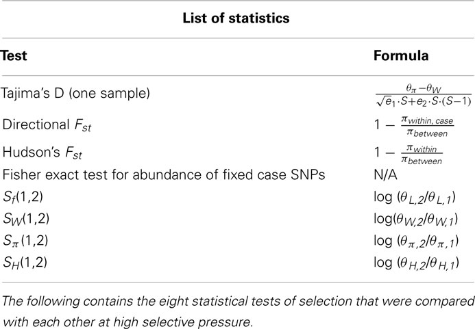
Table 1. List of statistics used.

2.2. Forward Simulation

We built a simulator that captured aspects of the pooled, diploid Drosophila populations described below. There are several different parameters for this simulator.

In a typical laboratory setting, a small group of individuals is used as a founder population. The simulator first has to generate this founder population before the application of selective pressure. In other words, this is a forward simulator that can be thought of as having three stages: (1) generation of a diverse founder population, (2) institution of a population bottleneck (to create the founder individuals) and introduction of the beneficial mutation, and (3) population expansion, followed by application of selection pressure (see Figure A6 in Appendix overview). Within each stage, a Wright-Fisher model with defined population size and time (in generations) is used. Parameters that are characteristic of the species, such as the per-base mutation and recombination rates, are set to be identical across all stages. With the Drosophila studies and most of the simulations, the per-base mutation rate (8.5 × 10⁻⁴/bp) was taken from Watterson’s estimator applied to the C1 population, while the per-base recombination rate was taken from Fiston-Lavier et al. (2010) to be 1.892 × 10⁻⁸/bp.

Since we do not know the genotypes or the relative differences between the individuals that spawned the biological populations, we simulate differences by generating a known “reference” haplotype and setting 2000 individuals to have two copies of this haplotype. As per coalescent theory, a neutrally evolving population of size 2000 will have a shared common ancestor after approximately 4000 generations (Kingman, 1982). We thus ran the simulator for 14000 generations to ensure that this criterion is met. As a result, this process generates a population based on a known reference, but each individual is sufficiently different from the reference as well as other individuals in the population.

After this, a 54-haplotype founder population is taken from the pool of genotypes. The beneficial mutation is introduced into exactly one of the founders, and the population is then immediately separated into two sets of 2000 individuals derived from these founders. At this stage, the selective pressure is applied to one of the sets, and the populations are allowed to evolve independently at constant size, usually for 200 generations. As far as measuring signal, we need to capture regions large enough to accurately estimate the true tree topology, yet small enough such that the signal is not masked by recombinations. Fixed window sizes (generally 50 kbp) are used for θ calculations, and the beneficial mutation is located exactly in the middle of these windows. The beneficial mutation is defined by two parameters: selection coefficient, s; and degree of dominance, h. The relative fitness of homozygous wild-type individuals is 1, heterozygous individuals is 1 + hs, and homozygous mutant individuals is 1 + s. s is generally variable, but h is fixed to be 0.5 in all trials. Parameters involved in the sequencing stage include sequencing sample size (generally 200 individuals), sequencing coverage (generally 70×), and base-calling error rates (generally 1%). The default values are intended to be representative of typical experimental conditions, and as such, are derived from the hypoxia dataset (see Methods). Each trial is repeated 500 times to get a more complete picture of the behavior of the statistics.

2.3. Preprocessing

Assuming even a 1% sequencing error rate, it is unlikely that we would be able to distinguish low frequency variants from sequencing errors at reasonable levels of coverage. Since under the null model, the SNP frequencies would follow a similar distribution, we tossed out all SNPs with a minor allele frequency of less than 10% from consideration. In addition, this would lead to a potential gain of power, as many of the de novo mutations would initially have frequencies less than 10% (see Figure 1B). At least 10× read depth at a site was required to have enough reasonable confidence in its frequency. In addition, when the selective pressures are high, it is common to see no SNPs with minor allelic frequencies ≥10%, leading to θ estimates of 0. In order to take the log ratio, pseudocounts of 0.1 were added to both numerator and denominator.

FIGURE 1

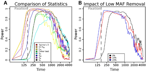
Figure 1. Power of different statistics as a function of time since bottleneck. (A) Power versus time plots for multiple statistics given a fixed selection pressure (s = 0.08). Statistics that weigh low frequency SNPs more, such as S_W, have a higher peak power, but decay faster. On the other hand, statistics that weigh high-frequency SNPs more, such as S_H, have a lower peak power, but retain power for a longer timespan. S_f (black, equal weights) and directional F_st (orange) both provide a reasonable compromise between peak power and duration. (B) The influence of removing low minor allelic frequency SNPs on the power of the S_f statistic. The black line represents the power of the S_f statistic at s = 0.08. Through tossing out low frequency SNPs (MAF < 10%, red curve and <20%, blue curve), we have a buffer from moderate error rates. As we weigh intermediate frequency SNP counts more, we have a slight gain of peak power, and this power is gained prior to fixation (as the extremely high-frequency SNPs are tossed out). However, the counts are lower and thus, more susceptible to noise, so we lose power over longer time spans. The red curve (10%) seems to provide a reasonable compromise between time and duration of high power.

With the application to Drosophila genotypes, it is possible that the phenotype impacts the mutation rate. For instance, it has been shown that temperature impacts mutation rate in Drosophila (Muller, 1928). Particularly in the regime well after fixation of the beneficial allele, we may see frequency spectrum differentials (and thus, false positives) only because of differences in de novo mutation counts. Under the assumption that the regions under selection are relatively small compared to the whole genome, if we take the genome as a whole, the effective population sizes of both populations should be similar. Adding an additive corrective factor, equivalent to log θ₁/θ₂ = μ₁/μ₂, where the θ values are computed for the entire genome, thus cancels the effect of mutation rate differences. In practice, this term was negligible for H1/C1, H2/C1, A1/N1, and A2/N1 calculations (see the following section for definitions).

2.4. Drosophila Datasets

We tested our method on two different sets of populations. In all cases, we apply the tests on a sliding window across the genome to identify regions under selection. The first involved populations of flies (D. melanogaster) originally reported in Zhou et al. (2007), and the selective pressure is manifested in normally lethal hypoxic (4%) environments. Starting from 27 isogenic lines, over a period of 200 generations, the oxygen concentration was gradually lowered from 8 to 4%. The controls consisted of flies originating from the same initial population growing for 200 generations under room air oxygen levels. Two biological replicates of both cases [H1 and H2, collectively called HT (hypoxia-tolerant) flies] and controls (C1 and C2) were derived from the same initial 27 lines. A stable population size of approximately 2000 flies resulted in each population, out of which 200 were pooled and sequenced at approximately 70× coverage per population. Previous work had indicated that this adaptation was genetic (or epigenetic) in nature.

The second represented populations undergoing sustained selection for accelerated development, and was described in Burke et al. (2010). The cases consisted of flies selected for an early reproduction (9–10 days per generation, instead of normal 14 day cycles). The cases (labeled as A1 and A2 here, collectively labeled as AD (accelerated development) flies) diverged from an ancestral population for approximately 600 generations, while the control (labeled as N1 here) were derived from the same ancestors, evolving for approximately 200 generations under 28 day cycles. All populations were sequenced at approximately 20× coverage. Although there was a high level of genetic concordance in replicate case populations, the authors did not find signatures of a classic selective sweep in the populations.

Following Holt et al. (2009), in a pooled population, for each SNP covered by r reads, the allelic frequency was estimated by a ratio of quality scores q_i of all bases spanning the SNP:

where x_i = 1 if read i has the derived allele. We used this approach instead of other weighting schemes presented in Holt et al. for the following reason: Let p_i equal the probability that a called read is accurate at a base. By definition, the quality score of a base-call is q_i ∝ −ln(1 − p_i) ; p_i (using the first-order approximation for the Maclaurin series). Then, the frequency of the derived allele can thus be approximated as

In other words, the frequency is estimated by down-weighting the contribution of allele calls for lower quality values.

We tested various metrics based on θ estimates on both real and simulated data. For all trials, the input consists of variations in two populations – one under positive selection and one under no selective pressure. Significant reductions in θ in the population under positive selection compared to the control population are viable candidates for further study.

2.5. Power and Significance Computations

The Type I error can be obtained by getting bounds on the tail probabilities of the distribution of the statistic in a scenario of no-selection. However, the distribution is not well understood, and is not normal. A quantile-quantile plot (Figures A4C,D in Appendix) suggests a strong deviation from the normal distribution for both statistics. If the underlying distribution is normal, the quantiles of the observed data would be linearly related to the quantiles of the standard normal distribution. As can be seen, this is not the case – the plots indicate fatter tails than expected. The Lilliefors test for normality (Lilliefors, 1967) quantifies the probabilities that any of these distributions are normal as P < 2.2 × 10⁻¹⁶. Therefore, we use empirical cut-offs for the statistics. To accurately determine Type I error, we use control vs control tests. In the simulations, we can replace the case population with a population evolving separately, but under identical conditions to the controls (for instance, under no selective pressure). In this situation, any deviation that appears to be significant is a false positive caused by genetic drift. To determine significance, we use a threshold corresponding to a 1% false positive rate from 500 control versus control simulations (in other words, the significance threshold was set at the fifth highest control vs control statistic value). For the Drosophila applications, we do not know the false positive rate, since there may be an unknown selective pressure acting on what we consider to be “controls”. In addition, some of the parameters we have assumed for the simulations (for instance, uniform coverage) may not hold throughout the genome. As a result, we utilize a biological replicate of the controls (such as C2 above) to determine a 1% false discovery rate (FDR) instead. To calculate this FDR, we calculate the fractions provided by the complementary CDFs of our statistics, applied across the genome for both control versus control and case versus control studies. We set the threshold of significance where the ratio of these fractions is roughly 1%. For instance, for the summed frequency statistic, a 1% FDR occurs when the threshold is set at 4 in both hypoxia populations mentioned above.

3. Results

3.1. Power Versus Time Under Different Measures of θ

To test the power of different statistics, we simulated case and control populations under fixed, high selection pressure (s = 0.08), and sampled n = 400 individuals from each (See Methods and Figure A6 in Appendix). For each test, power was determined as the fraction of cases with a test statistic more significant than a 1% FDR level cut-off determined in control versus control simulations. As Figure 1A shows, the power for all methods is high shortly after fixation of the beneficial mutation (at roughly t = 150 generations). However, if the populations are sampled at times prior to fixation (t < 150), or subsequent to it (t > 400), the different tests behave very differently. For example, F_st has relatively high power prior to fixation, but it decays subsequently, while S_H shows the opposite behavior. S_f shows at least 50% power over a wide range of generations (250–300). Interestingly, by removing sites with low minor allele frequencies, there is a shift in the power plot to earlier generations (Figure 1B).

To understand the reason for these trends, we plotted the mean scaled allele frequencies () for the case and control populations at t = 100,200,2000 generations after bottleneck (Figure 2). As mentioned earlier, Achaz (2009) showed that θ measures can be interpreted as linear combinations of these frequencies. A test of selection would have the most power when the chosen weights maximize the difference between the case and control populations. Under selective pressure, the lineage carrying the beneficial mutation expands rapidly, and we see an increase in intermediate to high-frequency alleles in regions under selection (Figure 2A). However, the frequency spectra are generally too close to distinguish at this stage, though, and most tests do not have high power. At fixation (Figure 2B), we see an almost complete loss of intermediate frequency SNPs. At this stage, the populations are well separable, and nearly any weighting can distinguish the two populations. Thus, most tests do well. However, as θ _π and θ _W weigh high-frequency alleles lower than lower frequencies, S_π and S_W show higher power than S_f (equal weights) and S_H (higher weight for high-frequency SNPs). Subsequent to fixation, with t ∈ [500,2000] (Figure 2C), the high-frequency alleles drift to fixation. However, we start seeing a fair number of de novo mutations at low frequencies. As a result, the best signal is obtained by methods that weigh low frequency alleles lower than high frequency (S_f, S_H).

FIGURE 2

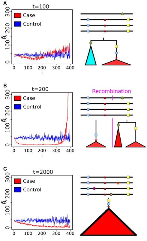
Figure 2. SNP frequency spectrum analysis. Scaled allele frequencies of simulated cases and control populations at different times after selection (s = 0.08). Here, ξ_i is the number of SNPs present in exactly i haplotypes. The ideal statistic is one that weighs alleles to maximize the separation between the blue and red line. (A) At t = 100, individuals with the beneficial mutation start to dominate the population (leading to a rise of high-frequency hitchhiking SNPs), but there is still a substantial fraction of individuals without the beneficial mutation. (B) At t = 200, many alleles that hitchhike with the beneficial mutation are near fixation, and the bulk of the mutations are very high frequency. Thus, measures that gives less weight to high-frequency alleles show high power. (C) At t = 2000, drift and recombination events decrease high-frequency alleles, while de novo mutations increase lower frequency. Thus, measures that weigh lower frequency alleles more rapidly lose power even with a clear signal between case and control.

Tajima’s D starts to lose power rapidly in the post-fixation regime. In addition, with this (or any other one sample test), we lose the benefit of a case-control setup, and we could lose power if there are any founder-specific or region-specific anomalies, which the simulator does not capture. The directional F_st generally performed well over a large time interval. Recall that the diversity in the case population is θ _π which weighs low frequency alleles higher than high-frequency alleles. It is not surprising that its power rises quickly, as the signal comes from differences between individual SNP frequencies between two populations. We only need to see a loss of diversity within a population (which occurs prior to fixation). As the intermediate frequency SNPs start to rise (around 1500 generations), power is maintained longer than S_π due to the large number of fixed SNPs in cases that increase the diversity between the case and control populations. However, in order to accurately determine π_between, we need a reasonably high subset of SNPs to be sampled in both populations. In circumstances where this may not be feasible (see below), this approach will be underpowered.

Pooling reduces the cost of sequencing, but loses exact information on haplotype frequencies. To test the corresponding loss of power due to lack of haplotype information, we computed the power of the S_f statistic on the underlying haplotypes and compared it to the corresponding power of sampling at 70× coverage, removing low frequency SNPs, and adding in 1% base-calling errors. The results (Figure 1B) suggest that even though we lose the ability to tell the exact frequencies, pooling does not have much impact on power. Assuming no sampling biases, the coverage is high enough such that we can accurately estimate the summed frequencies in a window. By removing SNPs with a minor allelic frequency of less than 10%, we gain peak power (since most de novo mutations in the cases get filtered out, leading to higher signal), but lose power as time goes on (as the SNP counts in both cases and controls become much lower, and thus, are more susceptible to noise). An additional benefit of filtering out low frequency SNPs is to dilute the impact of base-calling errors – due to the preprocessing, reasonable base-calling error rates barely influence the power.

Our results suggest that a variety of tests that use a case-control setup do well over different regimes of selection. We work with relatively high selection coefficients (s = 0.08) in these simulations, as it is often possible in model organism settings. By contrast, in naturally evolving populations, the selective pressure is usually lower and other tests might be better. We examine the impact of other parameters on power using the S_f and F_st statistics as exemplars.

3.1.1. Selection coefficient

According to coalescent theory, the time to the most recent common ancestor (MRCA) for a neutrally growing population with N haplotypes is 2N generations (Kingman, 1982). Under the assumption of a single beneficial mutation with viability 1 + s, the number of copies of the mutant allele will increase exponentially until fixation. Thus time to MRCA of a sample containing mutant alleles is similar to a coalescent under an exponentially growing populations, and scales as O(ln2Ns/s) (Campbell, 2007). The power of the test for selection will increase up to this point, as the separation between the two populations increases. Once the majority of the case populations have reached fixation (i.e., their MRCA is after the introduction of the beneficial mutation), however, de novo mutations subsequently reduce the power of the test. Some intuition can be provided in Figure 2. At the time that the beneficial mutation is close to the MRCA, the tree has a long main branch as lineages not carrying the mutation are less likely to survive. All of the mutations on the same linkage block as the beneficial mutation fall on the main branch of this tree and are consequently near fixation. Further, the branch lengths of the lineages descending from the main branch are reduced. Thus, the allele frequencies are dominated by sites having very low and very high frequencies, and we see relatively small numbers of sites with intermediate frequencies (Figure 2B). Thus, any statistic that scores the difference between the observed and expected (under neutral selection) will be at peak power near this time. However, different statistics measure this skew in different ways, and reach peak power at slightly different times. With further passage of time, more lineages come out, and the main branch becomes shorter, and the scaled frequency spectrum starts to match the neutral spectrum. Consequently, the power of all statistics reduces (Figure 2C).

We tested how power of each selection pressure was impacted by the number of generations that the populations were allowed to diverge after the bottleneck (Figure 3). The time to maximum power with the S_f statistic indeed scales according to ln2Ns/s (Figure A1 in Appendix), but reasonable power is achieved at a large number of generations. In all cases, the power drops rapidly at around N (2000) generations, disappearing at 2N generations. Additional trials of the impacts of coverage, base-calling error rate, founder population size, and sequencing sample size on S_f are in Figure A2 in Appendix. Given our population setup, around 20× pooled coverage is sufficient to achieve peak power. As mentioned earlier, the preprocessing provided tolerance to reasonable base-calling error rate. The population sample size seems to have minimal impact on power. The bottleneck has a fairly large impact, in large part because the beneficial mutation is introduced in exactly one haplotype. Thus, a large bottleneck size corresponds to a small initial frequency as well. Over 200 generations and relatively small selection pressure, the beneficial allele has not had sufficient time to fix in the population.

FIGURE 3

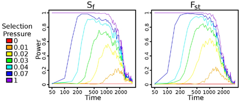
Figure 3. Power versus time after bottleneck. Power is calculated using a 1% false positive rate, as described in Section 2.5. Once a haplotype gets fixed in the population, the power increases rapidly for both statistics, although with slightly more power using F_st than using S_f. As time continues, though, the signal decays faster in F_st than in S_f, largely because the controls vary more sharply as time progresses.

3.2. Window Size

For model organism studies, we intend on determining regions under selection using a statistic on a sliding window of fixed size w. The choice of w may be important in determining the signature of selection. The overall per-window recombination rate (ρ′ = ρ·w) and mutation rate (μ′ = ρ·μ) increase linearly with increasing window size, directly influencing the power of the statistic.

Figure 4 plots, as contours, the power of S_f and F_st as a function of ρ′ and μ′. In general, the power increases with an increase in the mutation rate, as the selective sweep becomes easier to distinguish from genetic drift with a larger number of linked mutations. However, a very high mutation rate could create too many de novo mutations that mask the selection signature, leading to a reduction in power. In a similar fashion, the power increases with decreasing recombination rates, as recombination events increase the genetic diversity in the region.

FIGURE 4

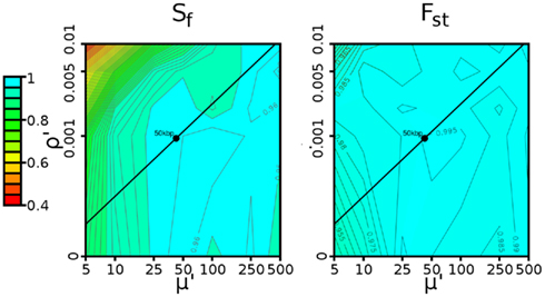
Figure 4. Contour plot describing determination of window size. The power of the (left) S_f and (right) F_st statistics for various combinations of recombination rate (ρ′ = ρ·w) and mutation rate (μ′ = μ·w). In both cases, the selection pressure was 0.08 (strong), and thresholds were defined by a 1% false positive rate, as described in Section 2.5. The black line represents the range of possible values caused by varying the window size in Drosophila. The black circle represents the 50-kbp window size ultimately chosen, which shows high (≥95%) power for both S_f and F_st.

The mutation and recombination rates both depend on factors such as sequence complexity, but we can estimate the average per-base rates. For Drosophila, the per-base mutation rate (8.5 × 10⁻⁴/bp) was taken from Watterson’s estimator applied to the C1 population (defined in Materials and Methods), while the per-base recombination rate was taken from Fiston-Lavier et al. (2010) to be 1.892 × 10⁻⁸/bp. If we treat the ratio of mutation to recombination rate as constant (μ′/ρ′ = μ/ρ ≈ 44926), varying the window size yields the black lines in these diagrams. Both statistics are robust to a wide range of window sizes. For w = 50 kbp (shown by the black circle in Figure 4), we have more than 95% power. As a result, we use 50 kbp windows in all trials.

3.3. Application to Drosophila Data

As mentioned in the Methods section, the specific thresholds set by the simulation may not be appropriate when dealing with Drosophila data. In order to determine the extent of deviation the experimental Drosophila populations, we estimated False Discovery Rate using the two control populations C2 and C1. Compared to the control versus control simulations (Figures A4A,B in Appendix), S_f (C2, C1) has six times the variance of the simulated data (Var (Drosophila) = 0.234, Var (simulated) = 0.041). As a result, we shifted the threshold for significance up to 4 (which corresponds to a 1% FDR for both S_f (H1, C1) and S_f (H2, C1) compared to S_f (C2, C1)). Additionally, sampling issues in the populations lead to many sites being undersampled. For example, of all variant sites in C1, almost 2/3 have a coverage of less than 10× in C2 (Figure A5 in Appendix). There was no major bias for any chromosome or large region, however. In this situation, for a statistic like F_st, both numerator and denominator are significantly impacted by this coverage differential. The value of π_within is directly related to the number of variants that are adequately sampled – if we assume that 2/3 of the average 50 kbp region has less than 10× coverage, we are effectively calculating the properties of a 17-kbp region. If we toss out the C1 variants that are not adequately covered in C2, the π_between would be similarly undersampled. If we keep these sites, the π_between calculation would need to be corrected, and the correction is non-trivial to define. Potentially, the net effect result is an underpowered statistic. Since S_f had generally similar power over many regimes, we decided to use S_f (with the global correction mentioned in the Methods) for our tests.

As shown in Figure 5A, the Hypoxia-tolerant (HT) flies showed strong, reproducible signals (see also Zhou et al., 2011). S_f (H1,C1) showed 2,480,272 bps in regions under selection, concentrated on the X and 3R chromosomes. The second hypoxia population, H2, also showed significant S_f (H2,C1) values in 2,035,013 bp. By contrast, S_f (C2,C1) (control to control) showed only 127,121 bps to be significant. Remarkably, a high fraction of the selected regions (1,509,436 bps) were shared by both populations, and the SNPs in the hypoxia-selected individuals were almost completely identical in these regions. Ninety-three percentage of the “fixed” SNPs were shared between H1 and H2 in the regions under selection, compared to 78% genome-wide, a hypergeometric P-value of 3.3.12 × 10⁻⁴³. This strongly suggests the same selective sweeps occurring in both populations. There were 24 common, distinct regions containing 188 genes. Indeed, a large number of genes in the selected region belonged to the Notch pathway, and additional experiments validated the essential role of the pathway for hypoxia tolerance (Zhou et al., 2011). It is likely that other experiments will clarify the roles of other genes in the selected regions.

FIGURE 5

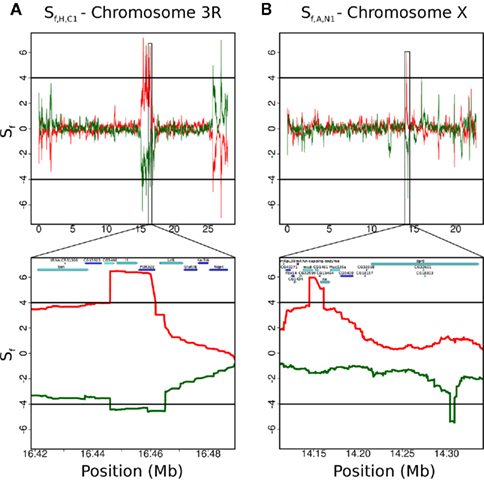
Figure 5. Comparison of S_f statistics in two different datasets. The plots show the S_f statistic for two biological replicates of case (one in red, the other flipped, in green) versus control. The black lines (at 4 for the red curve and −4 for the green curve) represent a threshold corresponding to a 1% FDR. (A) The S_f signal on the 3R chromosome shows strong concordance between the two hypoxia-tolerant populations, H1 (red) and H2 (green, flipped). The control in both cases is the C1 population. This implies that the same series of selective sweeps has occurred in both populations. (B) The two populations selected for accelerated development, A1 (red) and A2 (green, flipped), do not show strong concordance – even the significant regions that appear on a broad view to be colocated (such as around 14 Mb on chromosome X) do not match up. The control in both cases is the N1 population. This could be due to weaker selection pressure, lower coverages, or differences in generation times, among others.

By contrast, independently evolving AD flies did not show much similarity between populations. S_f (A1,N1) showed only 182,514 bps that were significant, while S_f (A2,N1) had 716,305 bps in regions under selection. Although some of the windows were situated in similar locations (Figure 5B), there is no overlap at the nucleotide level. This seemingly weak signal could be due to several reasons. Primarily, the selective pressure could be weaker. In this situation, it would take longer for the beneficial mutation to get fixed in the population. If the case population was sampled prior to fixation of the beneficial allele, our statistics would not show any power. Even if fixation has occurred, recombination events would reduce the size of the fixed LD block, and weaken the signal. Additionally, the cases were separated from the founder population for 600 generations, three times more than the controls as well as the hypoxia-tolerant populations. After the beneficial allele gets fixed in the population, any additional time of evolution would just cause de novo mutations to occur in the region under question, weakening the signal. Finally, it is possible that our preprocessing step of 10× minimum read depth for a SNP coupled with an average coverage of 20× could lead to overlooking signals in poorly covered regions. However, reducing the minimum read depth to 1× does not significantly impact the plots. Finally, the accelerated development phenotype may be defined loosely, having many genetic and epigenetic markers independently influencing the trait.

The two experiments illustrate the power and challenges of the technique. The selective pressure of hypoxia is strong, and leads to a clear signal, without the need for labor-intensive crosses. Moreover, the genetic basis of hypoxia adaptation is possibly constrained to a small subset of genes, and is conserved in two independent replicates. On the other hand, the signal for the “accelerated development” phenotype is weaker and possibly has multiple genetic determinants, allowing different loci to contribute to selection in the two independent populations.

4. Discussion

Our test shows great promise in identifying signatures of selection. The results suggest an economical, yet effective, approach for utilizing the capabilities of whole-genome sequencing to identify genetic determinants of phenotypes. The method requires that the phenotypes be used as a basis for laboratory selection and that the genomic data of the selected population be tested for signatures of selection. However, the test does not require high levels of sequencing to have full power. 20–30× pooled read depth per population was sufficient in our simulations; for typical model organisms with small genomes, this is relatively inexpensive.

In addition, the test provides higher resolution than genetic crosses and does not require a second level of sequencing to identify causal variants. For instance, let us take the cross-based protocol described in Leips and Mackay (2000). In this protocol, F1 offspring between two Drosophila strains are backcrossed to the parental line without the beneficial mutation. The resulting offspring are interbred for four generations, and then 98 recombinant inbred lines are created (which takes 25 more generations). In the paper, the QTL region sizes range from roughly 100 kbp to 3 Mbp. Our approach does not require the labor associated with constructing the cross and maintaining the RI lines, and we can easily reduce the LD block size further by two main mechanisms: increasing the number of generations that the populations are allowed to mix and increasing the initial genetic diversity (for instance, by increasing the number of parental strains).

At the same time, the test may not be universally applicable. Not all phenotypes present a strong selection pressure, and weak selection results in a weak signature. However, our empirical data in the scaled allele frequency spectrum provides a strong theoretical foundation for when a specific test might be effective, and the difference between the scaled allele frequencies of regions under selection versus controls suggest alternative tests that will be explored in the future. Furthermore, with dropping sequencing costs, it may be feasible to test the population at many time points during evolution, and develop tests of selection that also look at trends in the scaled allele frequency spectrum over time. Recently, tests have been developed for testing recent selection events, using long range haplotypes and other signals (Sabeti et al., 2002). We plan to develop analogs for pooled data to improve the power of the statistic for recent selection events. For older selection events, we plan on improving the statistics by using tests that depend upon an excess of coding and functional variants.

The test would work best given the sequences of a second control population (such as C2 above), so that a more accurate null distribution can be determined. In the absence of this, we can estimate the null distribution either via simulations or by assuming that the bulk of the genome is not under selection and using genomic control. Also, we determined that 50 kbp windows were appropriate by determining that an average window (as determined by per-base estimates of mutation and recombination rate) of this size has high power (see Figure 4). Not all regions of the genome are equivalent, though. For instance, if we assume that a recombination hotspot has the same properties as a typical region of the genome, we might overestimate the homogeneity of the region encompassed by the selective sweep. If we have an accurate recombination map, it would be beneficial to improve this by adjusting the window size (and significance threshold) based on location. In the absence of this, an alternate approach would entail running these tests over multiple window sizes. In this scenario, we would determine significance based on the presumed window size.

The statistic can potentially be applied to naturally occurring (or industrial) strains of organisms that have been evolving independently under different selective constraints, and even human populations. However, the lack of proper controls in naturally evolving sub-populations, will possibly require additional tests to associate the genetic signatures with the appropriate phenotypes. In this case, factors such as the time of divergence and isolation of sub-populations will also need to be considered. Development of these ideas will provide us with new tools for associating genotypes and phenotypes.

Conflict of Interest Statement

The authors declare that the research was conducted in the absence of any commercial or financial relationships that could be construed as a potential conflict of interest.

Acknowledgments

This work was supported by the National Science Foundation (NSF-III-0810905 and NSF-CCF-1115206); the National Human Genome Research Institute (5R01HG004962); the Eunice Kennedy Shriver National Institute of Child Health and Human Development (5P01HD032573); the National Institute of Neurological Disorders and Stroke (5R01NS037756); and an American Heart Association Award (0835188N).

References

Achaz, G. (2009). Frequency spectrum neutrality tests: one for all and all for one. Genetics 183, 249–258.

Pubmed Abstract | Pubmed Full Text | CrossRef Full Text

Bhatia, G., Bansal, V., Harismendy, O., Schork, N. J., Topol, E. J., Frazer, K., and Bafna, V. (2010). A covering method for detecting genetic associations between rare variants and common phenotypes. PLoS Comput. Biol. 6, e1000954. doi: 10.1371/journal.pcbi.1000954

Pubmed Abstract | Pubmed Full Text | CrossRef Full Text

Burke, M. K., Dunham, J. P., Shahrestani, P., Thornton, K. R., Rose, M. R., and Long, A. D. (2010). Genome-wide analysis of a long-term evolution experiment with Drosophila. Nature 467, 587–590.

Pubmed Abstract | Pubmed Full Text | CrossRef Full Text

Campbell, R. B. (2007). Coalescent size versus coalescent time with strong selection. Bull. Math. Biol. 69, 2249–2259.

Pubmed Abstract | Pubmed Full Text | CrossRef Full Text

Durrett, R. (2002). Probability Models for DNA Sequence Evolution, 2nd Edn. New York, NY: Springer-Verlag.

Fay, J. C., and Wu, C. I. (2000). Hitchhiking under positive Darwinian selection. Genetics 155, 1405–1413.

Pubmed Abstract | Pubmed Full Text

Fiston-Lavier, A. S., Singh, N. D., Lipatov, M., and Petrov, D. A. (2010). Drosophila melanogaster recombination rate calculator. Gene 463, 18–20.

Pubmed Abstract | Pubmed Full Text | CrossRef Full Text

Fu, Y. X. (1995). Statistical properties of segregating sites. Theor. Popul. Biol. 48, 172–197.

Pubmed Abstract | Pubmed Full Text | CrossRef Full Text

Fu, Y. X., and Huai, H. (2003). Estimating mutation rate: how to count mutations? Genetics 164, 797–805.

Pubmed Abstract | Pubmed Full Text

Fu, Y. X., and Li, W. H. (1993). Statistical tests of neutrality of mutations. Genetics 133, 693–709.

Pubmed Abstract | Pubmed Full Text

Holt, K. E., Teo, Y. Y., Li, H., Nair, S., Dougan, G., Wain, J., and Parkhill, J. (2009). Detecting SNPs and estimating allele frequencies in clonal bacterial populations by sequencing pooled DNA. Bioinformatics 25, 2074–2075.

Pubmed Abstract | Pubmed Full Text | CrossRef Full Text

Hudson, R. R., Slatkin, M., and Maddison, W. P. (1992). Estimation of levels of gene flow from DNA sequence data. Genetics 132, 583–589.

Pubmed Abstract | Pubmed Full Text

Kingman, J. F. C. (1982). On the genealogy of large populations. J. Appl. Probab. 19, 27–43.

CrossRef Full Text

Leips, J., and Mackay, T. F. C. (2000). Quantitative trait loci for life span in Drosophila melanogaster: interactions with genetic background and larval density. Genetics 155, 1773–1788.

Pubmed Abstract | Pubmed Full Text

Lilliefors, H. (1967). On the Kolmogorov-Smirnov Test for normality with mean and variance unknown. J. Am. Stat. Assoc. 62, 399–402.

CrossRef Full Text

Madsen, B. E., and Browning, S. R. (2009). A groupwise association test for rare mutations using a weighted sum statistic. PLoS Genet. 5, e1000384. doi: 10.1371/journal.pgen.1000384

Pubmed Abstract | Pubmed Full Text | CrossRef Full Text

Muller, H. J. (1928). The measurement of gene mutation rate in Drosophila, its high variability, and its dependence upon temperature. Genetics 13, 279–357.

Pubmed Abstract | Pubmed Full Text

Neale, B. M., Rivas, M. A., Voight, B. F., Altshuler, D., Devlin, B., Orho-Melander, M., Kathiresan, S., Purcell, S. M., Roeder, K., and Daly, M. J. (2011). Testing for an unusual distribution of rare variants. PLoS Genet. 7, e1001322. doi: 10.1371/journal.pgen.1001322

Pubmed Abstract | Pubmed Full Text | CrossRef Full Text

Sabeti, P. C., Reich, D. E., Higgins, J. M., Levine, H. Z., Richter, D. J., Schaffner, S. F., Gabriel, S. B., Platko, J. V., Patterson, N. J., McDonald, G. J., Ackerman, H. C., Campbell, S. J., Altshuler, D., Cooper, R., Kwiatkowski, D., Ward, R., and Lander, E. S. (2002). Detecting recent positive selection in the human genome from haplotype structure. Nature 419, 832–837.

Pubmed Abstract | Pubmed Full Text | CrossRef Full Text

Tajima, F. (1989). Statistical method for testing the neutral mutation hypothesis by DNA polymorphism. Genetics 123, 585–595.

Pubmed Abstract | Pubmed Full Text

Watterson, G. A. (1975). On the number of segregating sites in genetical models without recombination. Theor. Popul. Biol. 7, 256–276.

Pubmed Abstract | Pubmed Full Text | CrossRef Full Text

Wu, M. C., Lee, S., Cai, T., Li, Y., Boehnke, M., and Lin, X. (2011). Rare-variant association testing for sequencing data with the sequence kernel association test. Am. J. Hum. Genet. 89, 82–93.

Pubmed Abstract | Pubmed Full Text | CrossRef Full Text

Zhou, D., Udpa, N., Gersten, M., Visk, D. W., Bashir, A., Xue, J., Frazer, K. A., Posakony, J. W., Subramaniam, S., Bafna, V., and Haddad, G. G. (2011). Experimental selection of hypoxia-tolerant Drosophila melanogaster. Proc. Natl. Acad. Sci. U.S.A. 108, 2349–2354.

Pubmed Abstract | Pubmed Full Text | CrossRef Full Text

Zhou, D., Xue, J., Chen, J., Morcillo, P., Lambert, J. D., White, K. P., and Haddad, G. G. (2007). Experimental selection for Drosophila survival in extremely low O(2) environment. PLoS ONE 2, e490. doi: 10.1371/journal.pone.0000490

Pubmed Abstract | Pubmed Full Text | CrossRef Full Text

Appendix

FIGURE A1

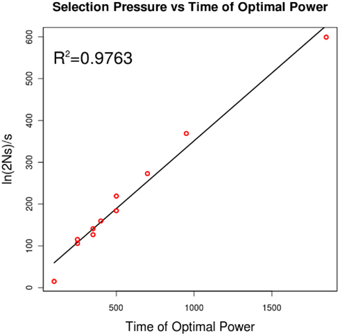
Figure A1. The relationship of selection pressure to the time of optimal power. Campbell (2007) has shown that, under strong selection, the expected time to fixation can be approximated by ln (2Ns)/s. This plot shows that, for a selection pressure s, the time that yields optimal power is linearly related to this quantity.

FIGURE A2

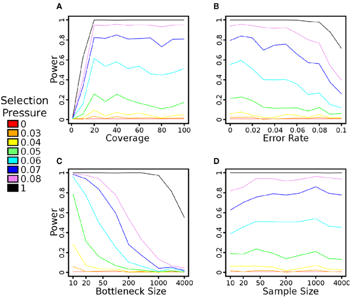
Figure A2. The impact of simulator parameters on the power of the S_f statistic. All trials were performed at 200 generations after the application of selection pressure and with all other simulator parameters as default, as per the Methods. A 1% false positive rate is also used to identify significance, as described in the Methods. (A) The impact of average read depth on power. As can be seen, approximately 20–30× coverage per population is sufficient to achieve maximal power. (B) The impact of base-calling error rates on power. Due to the removal of SNPs with less than 10% MAF, the statistic is robust to reasonable levels of error. (C) The impact of founder population size on power. The beneficial allele is present in exactly one haplotype in each setting, so this also represents the impact of the beneficial allele’s initial frequency on power. As expected, a low initial frequency (and high initial haplotype diversity) leads to a loss of power. (D) The impact of sequencing sample size on power. This parameter does not have a major impact on power – even 10 individuals are sufficient to determine signatures of selection in the population.

FIGURE A3

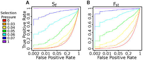
Figure A3. ROC Curve evaluating the impact of threshold on true positive and false positive rates. Using F_st leads to better performance than using S_f in this regime. For instance, at s = 0.05, with a 5% false positive rate, we can detect 33.8% of the true positives with S_f and 61.4% with F_st.

FIGURE A4

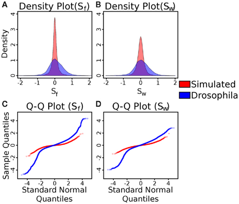
Figure A4. Tests of the distributions of the S_f and S_W statistics in simulated and Drosophila (C1 and C2) control versus control data. (A) Density plots of simulated (red) and Drosophila (blue) control S_f data (blue). (B) Density plots of simulated (red) and Drosophila (blue) control S_W data. As can be seen in both cases, with C1 and C2, the variance of the statistic is much higher than in the simulated control data. (C) Quantile-quantile plots of simulated (red) and Drosophila (blue) control S_f data, compared to a standard normal distribution. (D) Quantile-quantile plots of simulated (red) and Drosophila (blue) control S_W data, compared to a standard normal distribution. In these plots, a straight line indicates that the data comes from a normal distribution. In all cases, the plots indicate a non-normal distribution (quantified by the Lilliefors test for normality as having P-values less than 2.2 × 10⁻¹⁶).

FIGURE A5

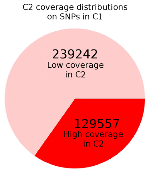
Figure A5. The overlap between well-covered SNPs in control populations C1 and C2. For all sites labeled as variant with more than 10× coverage in C1, we checked the corresponding coverage in C2. As can be seen, approximately 2/3 of these sites have “low” coverage of less than 10× in C2, perhaps due to library biases in the latter. Since we set a 10× minimum coverage threshold to ensure some level of precision on frequencies, these SNPs are not considered in C2. As a result, the π_between term used in the directional F_st is relatively underpowered. As the simulations showed that the powers of the statistics are fairly similar after fixation, we switched to S_f for the Drosophila applications.

FIGURE A6

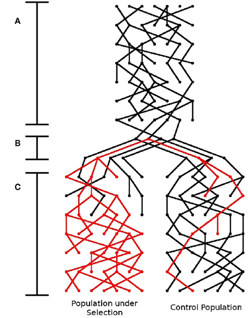
Figure A6. Schematic of simulator. There are three stages to this simulator: (A) Generation of founder population, (B) Shrinking of population to “founders,” introduction of the beneficial mutation (represented by the red lineage), and separation into sub-populations, and (C) Application of selection pressure in one subpopulation and expansion.