Statistical Inference and Reverse Engineering of Gene Regulatory Networks from Observational Expression Data

Emmert-Streib, Frank; Glazko, Galina; G¨okmen, Altay; De Matos Simoes, Ricardo

doi:10.3389/fgene.2012.00008

REVIEW article

Front. Genet., 03 February 2012

Sec. Computational Genomics

Volume 3 - 2012 | https://doi.org/10.3389/fgene.2012.00008

Statistical Inference and Reverse Engineering of Gene Regulatory Networks from Observational Expression Data

Frank Emmert-Streib^1,2*

Galina V. Glazko³*

Gökmen Altay^1,4,5

Ricardo de Matos Simoes¹

¹ Computational Biology and Machine Learning Lab, School of Medicine, Dentistry and Biomedical Sciences, Center for Cancer Research and Cell Biology, Queen’s University Belfast, Belfast, UK
² Statistics and Computational Biology Laboratory, Li Ka Shing Centre, Cancer Research UK Cambridge Research Institute, University of Cambridge, Cambridge, UK
³ Division of Biomedical Informatics, University of Arkansas for Medical Sciences, Little Rock, AR, USA
⁴ Department of Oncology, Cancer Research UK Cambridge Research Institute, University of Cambridge, Cambridge, UK
⁵ Department of Electrical and Electronics Engineering, Bahcesehir University, Istanbul, Turkey

In this paper, we present a systematic and conceptual overview of methods for inferring gene regulatory networks from observational gene expression data. Further, we discuss two classic approaches to infer causal structures and compare them with contemporary methods by providing a conceptual categorization thereof. We complement the above by surveying global and local evaluation measures for assessing the performance of inference algorithms.

1. Introduction

The purpose of this paper is to provide a systematic overview of methods used to estimate gene regulatory networks (GRN) from large-scale expression data. The inference of gene regulatory networks, which is sometimes also referred to as reverse engineering (Stolovitzky and Califano, 2007; Stolovitzky et al., 2009), is the process of estimating the direct physical (biochemical) interactions of a cellular system from data. That means one aims for identifying all molecular regulatory interactions among genes that are present in an organism to establish and maintain all required biological functions characterizing a certain physiological state of a cell. Depending on the data used for inferring the network, which, principally, may either come from DNA microarray, RNA-seq, proteomics or ChIP-chip experiments, or combinations thereof, the biological interpretation of an edge in these networks is dependent thereon. For expression data, inferred interactions may preferably indicate transcription regulation, but can also correspond to protein-protein interactions. Due to the causal character of these networks, which ensures a meaningful biological interpretation, the genome-wide inference of gene regulatory networks holds great promise in enhancing the understanding of normal cell physiology, and also complex pathological phenotypes (Barabási and Oltvai, 2004; Emmert-Streib, 2007; Schadt, 2009).

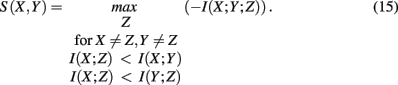
Due to the fact that this field is currently vastly expanding, this overview is inevitably incomplete. Instead of aiming to cover as many approaches as possible, we focus on conceptual clarity and methods for observational expression data. That means, we review statistical approaches from the literature we consider most important and show that they can be categorized nicely according to assumptions they make about the dynamic behavior of the data but also with respect to conceptual strategies they employ. In order to facilitate the understanding of the latter point we present also two seminal, and in the meanwhile classic, methods for the causal inference of networks and their theoretical foundations (Chow and Liu, 1968; Pearl, 1988; Spirtes et al., 1993). Model-based approaches based on, e.g., Boolean networks or differential equations (de Jong, 2002; Liu et al., 2008) are not covered in this paper. Also, supervised and semi-supervised network inference methods (Ernst et al., 2008; Mordelet and Vert, 2008; Cerulo et al., 2010) that require a training set will not be discussed. Further, we content ourselves with approaches for observational data (Rubin, 1974; Rosenbaum, 2002) neglecting methods that utilize interventional or perturbational data. In addition to the presentation of inference methods, we provide also an overview of global and local performance metrics frequently used to assess the inference abilities of such methods. Finally, we will emphasize and discuss the conceptual closeness of all current methods with respect to two classic methods (Chow and Liu, 1968; Pearl, 1988; Spirtes et al., 1993).

2. Methods

The inference of gene networks from high-throughput data is a very complex and vastly expanding area triggered by the invention of measurement technologies. In order to provide a systematic discussion of the underlying principles we limit this review to observational, steady-state gene expression data, and consider correlation- and mutual information-based inference methods only, as visualized in Figure 1. These methods are representative of linear and non-linear methods. Principally, there are three fundamental levels of a molecular system as given by the central dogma of molecular biology (Crick, 1970), namely, the DNA, mRNA, and the protein level. Consequently, these levels imply sensible variables that can and should be measured to obtain information about the biological function of a cell. Specifically, one can distinguish between measurements that provide information about the protein-DNA binding (ChIP-chip, ChIP-seq), gene expression (DNA microarray, RNA-seq), and the protein-protein interaction (protein microarray) which can be used to infer various types of gene networks (Emmert-Streib and Glazko, 2011). We focus in this review on observational gene expression data because to date, this data type is predominating.

FIGURE 1

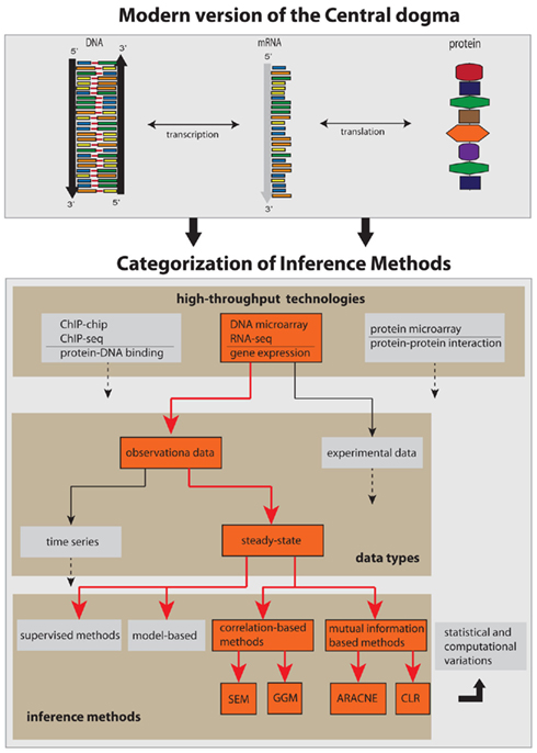
Figure 1. Conceptual categorization of network inference methods and the biology, technology, and data types they depend on. The red arrows and boxes represent the focus of this review article.

The complexity of the network inference problem can be visualized with the help of Figure 1. There are two major factors that contribute to it. First, almost all components shown in Figure 1 as represented by the boxes can be connected with each other. That means, they are not mutually exclusive but can be combined in a great variety. This concerns the integration of different high-throughput data, but also the combination of different data types or even methods. Second, any network inference method is subject to statistical and computational variations in form of technical modifications. This may relate to newly developed statistical estimators or optimization methods, or to the design of efficient algorithms or their parallelization on a computer cluster.

2.1. Classic Approaches to Causal Inference

We begin our presentation by some necessary preliminaries. Directed acyclic graphs (DAGs) are frequently employed to represent causal relations among variables (Wright, 1934; Verma and Pearl, 1990; Shipley, 2000). In such a graph, G, a directed edge from node X to Y means that X is the cause for Y. For this reason these networks are also called causal graphs. For the causal inference of network structures, the graph theoretical measure d-separation is key. It can be defined in the following way (Pearl, 1988; Verma and Pearl, 1990).

Definition 1. Two nodes X and Y are called d-separated by set S if and only if X, Y, and S are disjoint and every undirected path from X to Y is blocked by the nodes in set S.

If X is d-separated from Y by S we write (X ╨ Y|S).

Definition 2. A path w is called d-separated or blocked by a set of nodes S if and only if either of the following two criteria hold:

1. on w is a node s which is no collider and s ∈ S

2. on w is a node s which is a collider and it holds s ∉ S and de(s) ∉ S.

Here, de(s) denotes the set of descendants of node s. A node Z is called a collider if the edge of the incoming as well as the edge of the outgoing link point toward Z. In Figure 2 we clarify this notation. The top Figure shows a collider Z. For example, considering the path X → Z ← Y, then from the definition of d-separation follows that X is d-separated from Y if conditioned on the empty set S = ∅, (X ╨ Y|∅), or simply (X ╨ Y). However, if we condition on Z then (X yes Y|Z), according to Definition 2. In this case Z unblocks the path between X and Y. In the middle and bottom panels in Figure 2 two non-colliders (a chain and a fork) are shown. We want to notice that in general one node is sufficient to block a path.

FIGURE 2

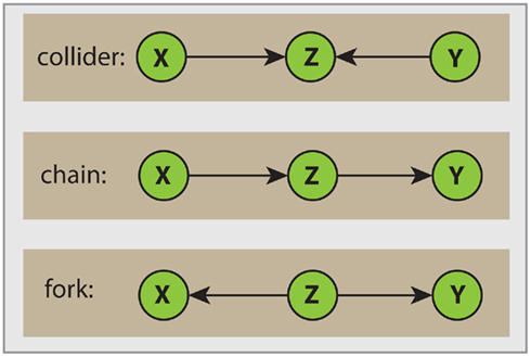
Figure 2. Visualization of different path types. The orientation of edges with respect to the node Z allow the following distinction. Top: collider; middle: chain; bottom: fork.

A systematic connection between independence relations among variables V forming a DAG, and a process in form of a probability distribution P, can be given with the help of d-separation and Markov independencies. Formally, this connection is provided by an I-map (independency map). A DAG G is called an I-map of P if

Here the subscript G refers to the structure represented by a DAG and the independence relations provided by d-separation, and a “P” refers to the probability distribution whereas the independence relations corresponds to conditional Markov independencies. From equation (1) follows the definition of a Bayesian network (Pearl, 1988).

Definition 3. Bayesian network Given a probability distribution P on a set of random variables V. A DAG, G = (V, E), is called a Bayesian network of P if and only if G is a minimal I-map of P.

Here minimal I-map means that if any edge in the DAG is deleted, G is no longer an I-map of P. There are alternative definitions of a Bayesian network (Pearl, 2000), however, the definition given above emphasizes its connection to d-separation best. This is important to emphasize because Bayesian networks are first of all about independence relations, and not about specific probability distributions.

In our opinion, there are basically two principle approaches in the literature that are relevant for our contextual problem, which proof mathematically that, under certain conditions, they are capable of systematically inferring causal relations. The first principle approach, which is based on d-separation, has been independently developed by two group; Verma and Pearl (1991) and Spirtes et al. (1993). The second principle approach is from Chow and Liu (1968). Certainly, there are various variations of these two approaches, however, in the following, we focus only on the essential principles of both methods.

The first algorithm we discuss proven to reconstruct a causal structure is the inductive causation (IC) algorithm. For simplicity, we assume causal sufficiency, which means that latent variables are absent. The IC algorithm starts with the construction of an undirected dependency graph (UDG) by testing exhaustively for the independence of variable X from Y given a set S_xy. Exhaustively means, for any set S_xy that can be formed among the available variables. We denote this by (X ╨ Y | S_xy)_P emphasizing explicitly that this independence is with respect to an underlying distribution P.

The basic principle on which the IC algorithm is based on, is a connection between the d-separation relations of a DAG G and independence relations of a probability distribution P consistent with the structure of the DAG G. The crucial point is that the distribution P and its independence relations are not given (known) but they need to be estimated from data, generated from the distribution P. Schematically, this is outlined in Figure 3. Here, the red line corresponds to the experimentally generation of the data, e.g., by means of DNA microarrays, and the blue line corresponds to the theoretical, however, unobservable (that’s why this line is dashed), independence relations present in the DAG G that can be expressed by the concept of d-separation. Based on the data, an inference method aims for estimating these independence relations statistically. The gray box marks the range of the inference method.

FIGURE 3

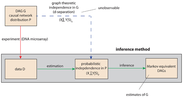
Figure 3. Schematic visualization of the importance of the d-separation concept in the inferential task to recover the structure of a DAG G. The red, green, and blue lines refer to experimental, inferential, or theoretical (unobservable) steps. For notational simplicity, we use also in the inferential step the symbol P instead of yes to indicate an estimate of P.

The second algorithm proven to reconstruct a causal structure is from Chow and Liu (1968). It is based on the MWST (maximum weight spanning tree) algorithm, which connects node pairs in a way that the resulting network structure forms a tree with a minimal sum of edge weights. It is of interest to note that the proof of the MWST algorithm (see for example Pearl, 1988) is based on the data processing inequality (DPI; Cover and Thomas, 1991), which will be discussed later in the paper for ARACNE.

2.2. Categorization of Methods

In this section we present an overview and a categorization of methods that have been specifically introduced to infer gene regulatory networks from observational gene expression data. Previously, there have been other reviews that attempted to do this (Werhli et al., 2006; Bansal et al., 2007; Margolin and Califano, 2007; Markowetz and Spang, 2007; Hache et al., 2009; Olsen et al., 2009; de Smet and Marchal, 2010; Penfold and Wild, 2011), however, their emphasis and conceptualization deviates from ours.

2.2.1. Correlation-based estimation methods

2.2.1.1 Co-expression networks. There are two principally different ways to construct co-expression networks from microarray data. One approach follows a hard- and the other a soft-thresholding of correlation coefficients (Zhou et al., 2002; Horvath and Dong, 2008). In the following r_ij = |cor(i,j)| is the absolute value of the Pearson correlation coefficient. In the case of hard-thresholding, the correlation coefficient r_ij between gene i and j is assessed with respect to a threshold τ and both genes are connected by an edge, A_ij = A_ji = 1, if r_ij ≥ τ, otherwise the genes remain unconnected, A_ij = A_ji = 0. The threshold or cut-off parameter τ can be obtained from randomization of the data allowing the assessment of statistical significance (Carter et al., 2004). This results in an undirected, unweighted network.

For the soft-thresholding two types of adjacency functions are frequently used (Zhang and Horvath, 2005). The sigmoid function,

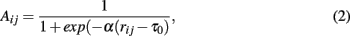
and the power adjacency function,

Both types of adjacency functions lead to undirected but weighted networks. In order to choose the above parameters appropriately Zhang and Horvath (2005) suggested to adjust them in a way that the resulting network has approximately a scale-free degree distribution.

We would like to remark that the purpose for the construction of co-expression networks is different to all other methods discussed in this paper. Co-expression networks serve as means to explore the functionality of genes on a systems level (Zhang and Horvath, 2005) and do not aim to be causal representations of regulatory networks. Nevertheless, we included them in this review to point out that also networks that are not causal can be very useful in gaining biological understanding and insights.

2.2.1.2 Asymmetric-N. Asymmetric-N is an algorithm that takes the fact into account that biological networks contain hubs. It is a modified version of Symmetric-N (Agrawal, 2002) which was designed for the construction of co-expression networks (Chen et al., 2008a). The two-step algorithm of Agrawal (2002), Symmetric-N, utilizes the N-nearest-neighbor concept. In a first step, for each node in the network its correlation to other nodes is calculated and sorted in descending order. In a second step, each pair of nodes is evaluated one by one and if for a pair of nodes both are in the corresponding N-nearest-neighbors list, a connection between them is included. Otherwise, they are not connected. Here N is a pre-defined cut-off value for the number of neighbor nodes to be considered (Agrawal, 2002). It is demonstrated in Agrawal (2002) that the inferred network has a scale-free topology.

Instead of using N neighbors for all nodes as potential connections, a higher number N_C is assigned to some core nodes (e.g., TFs) and a smaller number N_P is assigned to periphery nodes (e.g., non-TFs). Since the numbers of potential neighbors are different for core and peripheral nodes, the algorithm was called Asymmetric-N (Chen et al., 2008a). Asymmetric-N employs the intuition that transcription factors (TFs) are more frequently connected to other genes than regulated genes. An interesting result found in Chen et al. (2008a) is that Asymmetric-N performed better than Bayesian networks for small sample sizes.

2.2.1.3 SEM (structural equation model). Xiong et al. (2004) use a structural equation model (SEM; Jöreskog, 1973; Bollen, 1989) to reconstruct gene networks. Structural equation models combine path analysis (Wright, 1921, 1934) and confirmatory factor analysis (Jöreskog, 1969; Brown, 2006).

Xiong et al.’s (2004) approach starts by assuming that the expression level of genes, X, can be described linearly by

Here X is a vector of p endogenous and ξ a vector of q exogenous variables, and B and Γ are p × p respectively p × q coupling matrices. The last term in equation (4), ε, represents noise. The structure of the regulatory gene network is coded by the entries of the coupling matrices B and Γ. The structural equation in equation (4) is learned in two steps. First, assuming the structure of the network is known the coupling parameters are estimated via maximum likelihood optimizing the distance between the (p + q) × (p + q) covariance matrix Σ(Θ) and the sample covariance matrix S estimated from the data. Here, Θ = f (B, Γ, Φ, Ψ), is a function of the parameters of the SEM and the covariances of ξ (Φ) and ε (Ψ) that can be expressed analytically. The second step consists in finding the network structure (of B and Γ) by an optimization method whereas the different models are assessed by Akaike’s information criterion (AIC).

2.2.1.4 Low-order partial correlation. Partial correlations of low-order have been employed in de la Fuente et al. (2004), Magwene and Kim (2004), Wille and Bühlmann (2006). This approach is capable to infer undirected networks only, because a correlation, of any order, is symmetric in its arguments. The principle working mechanism of this approach is as follows. Starting with a fully connected network, interactions between genes are iteratively excluded by moving toward an increasing order of the correlation coefficient. More specifically, starting from a fully connected adjacency matrix A, one calculates in the first step all pair-wise correlation coefficients, ρ_ij = ρ(X_i, X_j). If ρ_ij = 0 the connection between gene X_i and X_j is deleted, A_ij = A_ji = 0. Inthe second step all partial correlation coefficients of first-order, yes are calculated for all triplets of genes with ρ_ij ≠ 0. Now, if there is at least one gene X_k for which ρ_ij|k = 0 holds the connection between gene X_i and X_j is deleted, A_ij = A_ji = 0. Continuation to higher orders is analogously. The exclusion of interactions is based on testing the null hypothesis ρ_ij = 0 against the alternative hypothesis ρ_ij ≠ 0 for all orders of the (partial) correlation coefficients. In (de la Fuente et al., 2004) this approach was applied up to order three. The resulting network from this procedure is frequently called an undirected dependency graph (UDG; Shipley, 2000). An implementation of this approach is called ParCorA (de la Fuente et al., 2004).

2.2.1.5 GGM (graphical Gaussian model). GGM, also known as covariance selection model, concentration graph, or Markov random field (Dempster, 1972; Whittaker, 1990; Koller and Friedman, 2009), is a graphical model which assumes that all variables are distributed according to a multivariate normal distribution with a specific structure of the inverse of the covariance matrix, Ω = Σ⁻¹, also called precision or concentration matrix. Network inference methods based on GGM make use of the relation,

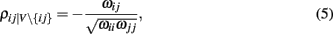
connecting the partial correlation of full-order with the elements of Ω, w_ij ∈ Ω. The partial correlation is of full-order (with respect to the number of genes) because V\{ij} is the set of all genes excluding i and j, i.e., the largest possible set of genes not considering i and j. In case of a vanishing partial correlation in equation (5) one can write

From this conditional independence relation, the principle way to infer a network structure from GGM becomes apparent estimating a network in the following way. If ρ_ij|V\{ij} ≠ 0, according to a hypothesis test, we include an edge, A_ij = A_ji = 1, otherwise there is no edge between i and j.

Several approaches have been made to infer gene regulatory networks based on GGM (Wille et al., 2004; Schäfer and Strimmer, 2005; Li and Gui, 2006). These methods differ in the way the inverse of the covariance matrix, Σ⁻¹, is estimated and in the statistical tests employed to define significance. The reason for these technical variants comes from a variety of problems. First, if the number of samples is smaller than the number of genes, which is typically the case for genomics data, the sample covariance matrix is not positive definite and, hence, not invertible. Another problem is caused by the small samples size problem (Schäfer and Strimmer, 2005).

2.2.1.6 BN (Bayesian networks). Bayesian networks allow identifying a DAG structure of a network. BN were among the first methods that have been applied to expression data to infer GRN (Friedman et al., 2000; Hartemink et al., 2001). In order to overcome the problem that only acyclic networks can be inferred by BN, which would be a severe limitation considering the fact that real biological networks contain many feedback loops and are, hence, cyclic, a modified method called dynamic Bayesian network (DBN) is used instead. Briefly, DBN unfold cyclic processes by mapping them onto a sequence of acyclic events, which can then be analyzed with a BN (Dean and Kanazawa, 1990; Koller and Friedman, 2009). For the inference of GRN, this approach has been applied in Husmeier (2003), Perrin et al. (2003), Zou and Conzen (2005). The variations in these approaches provide different methods for the structure learning problem, which is the integral part of a BN learned from data. Principally, a major practical problem of a BN is that the computational complexity of algorithms to learn their structure has been shown to be NP-hard for score-based approaches (Chickering et al., 1995; Chickering, 1996). Hence, BN or DBN can be either only applied to quite small networks or heuristic approximation methods have to be used that separate the score into tractable units that can be optimized by locally constraint search techniques making the computational complexity manageable (Friedman et al., 1999, 2000).

In Figure 6, we categorize BN as correlation-based methods because the simplest statistical realization of a BN is obtained by estimating (X ╨ Y|S)_P, see section 1, by means of partial correlation coefficients (Spirtes et al., 1993; Pearl, 2000). However, also non-linear approaches are possible.

2.2.2. Information-theory based estimation methods

In the following, we restrict our discussion to the working mechanisms of the discussed procedures. However, we want to emphasize that also for these methods the employed statistical estimators are of importance (Beirlant et al., 1997; Steuer et al., 2002; Daub et al., 2004; Kraskov et al., 2004; Khan et al., 2007).

2.2.2.1 A. Mutual information-based. RN (relevance networks). The principle idea of RN (Butte and Kohane, 2000) is to compute all mutual information (MI) values for all pairs of genes, for a given data set, and declare mutual information values as relevant if their corresponding value is larger than a given threshold I₀. The resulting network is constructed based on this threshold by including an edge between two genes in the respective adjacency matrix of the network, A_ij = A_ji = 1, if I_ij > I₀, otherwise no edge is included between i and j. In Butte and Kohane (2000) the threshold I₀ was found by randomization of the expression data set. From this randomization, mutual information values were re-calculated from which a reference distribution of mutual information values, resembling a null-distribution, was obtained. Based on this reference distribution the threshold I₀ was obtained by heuristic arguments. For this reason, mutual information values that are larger than I₀ are called relevant but cannot necessarily be called statistically significant.

ARACNE (algorithm for the reconstruction of accurate cellular networks). ARACNE (Basso et al., 2005; Margolin et al., 2006) is similar to RN because it also uses mutual information and a randomization of the data to obtain a threshold I₀ allowing to declare mutual information values significant if I_ij > I₀ ¹. If I_ij is found to be significant, than an edge is included in the corresponding adjacency matrix between gene i and j, A_ij = A_ji = 1, otherwise no edge is included. However, in contrast to RN, ARACNE performs a second step testing all gene-triplets (three genes with mutual information values larger than I₀) such that, for each triplet (ijk), the edge corresponding to the lowest mutual information value yes with (i′j′) = argmin{I_ij, I_jk, I_ik}, is eliminated from the adjacency matrix, if it is smaller than the second smallest MI value I₂ multiplied by a factor, i.e.,

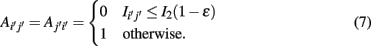
Here 0 ≤ ∈ ≤ 1. The introduction of this step has been motivated by the so called data processing inequality (DPI; Cover and Thomas, 1991). The DPI is a relation between mutual information values which means loosely that a post-processing of data cannot increase its information content. Specifically, one can show (Cover and Thomas, 1991) that the DPI for the following relation between the three random variables,

implies that I(X,Z) ≤ I(X,Y). Due to the fact that the criteria in equation (8) is for ∈ > 0 less stringent than the DPI [equation (9)], ∈ is called tolerance parameter.

To ensure that the application of equation (8) results in an unique solution, independent of the order the triples have been selected, the procedure starts by listing all possible triplets in the network G. Then all of these triplets are tested. Hence, the results of these tests have no influence on subsequent tests of triplets. At the end of the second step, the resulting network represents the final result.

ARACNE employs two parameters, I₀ and ∈. The cut-off parameter I₀ is determined by a resampling method estimating the distribution of the null hypothesis corresponding to a vanishing mutual information. This allows to assign p-values to mutual information values. In contrast, the DPI is not directly connected to statistical inference, but serves as a filtering step. Optimal values of ∈ are found from simulation studies that allow a comparison with the underlying true network. Hence, I₀ is found in an unsupervised and ∈ in a supervised way of learning.

CLR (context likelihood of relatedness). CLR (Faith et al., 2007) is also an extension of RN. It starts by estimating the pair-wise mutual information values for all genes. Then, CLR estimates the statistical likelihood of each MI value I_ij, for a particular pair of genes (ij), by comparing this MI value to a background. Specifically, for each gene pair (ij) two z-scores are obtained, one for gene i and one for gene j, by comparing the mutual information value I_ij with gene specific distributions, p_i and p_j. Here the two distributions p_i and p_j correspond to the distributions of mutual information values related to gene i ({I_ik|k ∈ V}) and gene j ({I_jk|k ∈ V}). By making a normality assumption about these distributions, corresponding z-scores, z_i and z_j, can be obtained from which the joint likelihood measure yes is calculated. In contrast to RN and ARACNE, which employ a global threshold I₀ for each mutual information value correspondingly pair of genes, CLR estimates individual thresholds by considering an individual background for each pair of genes. This procedure can be seen as a first attempt to take the network context of gene pairs into account.

C3NET (conservative causal core). C3NET consists of two main steps (Altay and Emmert-Streib, 2010a). The first step is for the elimination of non-significant edges, whereas the second step selects for each gene the edge among the remaining ones with maximum mutual in formation value. The first step is similar to RN (Butte and Kohane, 2000), ARACNE (Margolin et al., 2006), or CLR (Faith et al., 2007) essential for eliminating non-significant links, according to a chosen significance level α, between gene pairs. In the second step, the most significant link for each gene is selected. This link corresponds also to the highest MI value among the neighbor edges for each gene. This implies that the highest possible number of edges that can be inferred by C3NET is equal to the number of genes under consideration. This number can decrease for several reasons. For example, when two genes have the same edge with maximum MI value. In this case, the same edge would be chosen by both genes to be included in the network. However, if an edge is already present another inclusion does not lead to an additional edge. Another case corresponds to the situation when a gene does not have significant edges at all. In this case, apparently, no edge can be included in the network. Since C3NET employs MI values as test statistics among genes, there is no directional information that can be inferred thereof. Hence, the resulting network is undirected and unweighted. For a detailed explanation of C3NET and technical details, the reader is referred to Altay and Emmert-Streib(2010a, 2011), de Matos Simoes and Emmert-Streib (2011).

2.2.2.2 B. Extensions of mutual information and conditional mutual information. SA-CLR (synergy augmented CLR). As indicated by its name, SA-CLR is based on CLR but includes synergistic effects between genes (Anastassiou, 2007; Watkinson et al., 2009). Synergy,

is defined as the difference between the generalized two-way mutual information,

and the mutual information values for two random variables. A visualization of synergy is shown in Figure 4. In this figure, the different intersections of the three variables X, Y, and Z are labeled by lower case letters, whereas “e” corresponds to the synergy, Syn(X,Y;Z). Using the definitions of the occurring mutual information values one obtains a simplified form of the synergy, given by

FIGURE 4

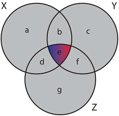
Figure 4. Generalized Venn diagram showing the synergy Syn(X,Y;Z) = − I(X;Y;Z). The synergy is shown in red and blue because it can assume positive as well as negative values.

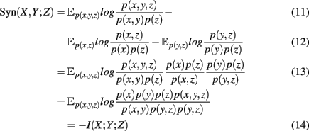
which is the negative of the three-dimensional interaction information (Watkinson et al., 2009). We want to remark that I(X; Y; Z) can assume positive as well as negative values (McGill, 1954). For this reason the intersection “e” in Figure 4 is shown in blue and red to emphasize this. Due to the fact that a Venn diagram visualizes logical relations between variables Figure 4 is no Venn diagram in the strict sense but a generalization thereof, allowing also to express negative values by including colors in the representation. The idea of SA-CLR consists in utilizing the synergy given in equation (10) in the following way,

This term is called synergistic regulation index (SRI; Watkinson et al., 2009). The interpretation of SRI is that for two given genes, X and Y, we are searching a third one, Z, that maximizes the synergy Syn(X, Y; Z) obeying the above constraints. This gene, Z, can be be arbitrarily chosen among all available genes, besides X and Y. The two constraints that involve mutual information, are chosen assuming that gene X and Z regulate Y. In this case, the mutual information between the two regulators, X and Z, should be smallest, motivating the constraints. Interestingly, these constraints introduce an asymmetry in X and Y² making it possible to speak about regulator and modulator genes. In the case of a positive synergy, a significant high value of SRI may indicate that gene X regulates genes Y (Watkinson et al., 2009).

In order to detect also non-cooperative effects, the measure actually used by SA-CLR is I(X, Y) + S(X, Y), the mutual information between two genes plus their synergistic regulation index. The significance of I(X, Y) + S(X, Y) is detected in a similar way as described above for CLR.

It is interesting to note that

holds formally but is not identical to the (general) conditional mutual information I(X; Y|Z) because the synergy for X, Y, and Z has to be positive. To make this clear, we included this constraint visibly in equation (20). This allows SA-CLR, in contrast to CLR, to obtain a directed network by assigning an edge from gene X to Y if I(X; Y) + S(X, Y) is significant.

MRNET (maximum relevance, minimum redundance). MRNET (Meyer et al., 2007) is an iterative algorithm that identifies potential interaction partners of a target gene Y that maximize a scoring function. Its working mechanism is as follows,

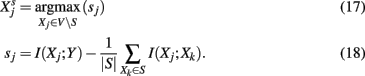
Whenever a gene, X_j, is found with a score that maximizes equation (21) and s_j is above a threshold, s₀, then this gene is added to the set S. The algorithm is iterated until no further gene can be found that would pass the threshold test. The basic idea of MRNET is to find interaction partners for Y that are of maximal relevance [first term in equation (22)] for Y, but introduce a minimum redundancy [second term in equation (22)] with respect to the already found interaction partners in the set S. Starting with a fully connected, undirected network among all genes, MRNET reduces successively edges between Y and V S, which have not maximized the score in equation 22.

We want to remark that the score s_j can be approximated by the difference between two mutual information values,

where the (auxiliary) random variable, A, represents the influence of the variables in the set S. Equation (23) is visualized in the left Figure 5. Here, I(X_j; Y) corresponds to “d” and I(X_j; A) to “b.” Due to the fact that the mutual information is always positive, I(X_j; Y) adds a positive and I(X_j; A) a negative value to s_j, indicated by blue and red colors. It has been argued in (Meyer et al., 2007) that due to the maximization of equation (22), MRNET approximates the conditional mutual information I(X_j;Y|S). This is also motivated by Figure 5.

FIGURE 5

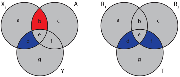
Figure 5. Generalized Venn diagrams of the information captured by different measures. Left: score s_j [equation (23)] for MRNET. Right: the MI₃ measure of the MI3 algorithm. Blue corresponds to positive and red to a negative values.

MI3 (mutual information 3). The MI3 algorithm (Luo et al., 2008) uses three-way mutual information for the inference, hypothesizing that gene regulation commonly involves more than one regulator genes. The value of the measure MI₃ is defined as,

which equals the difference of mutual informations between the target gene and the two regulators and the target gene with one of the regulators. Alternatively, MI₃ can also be written as

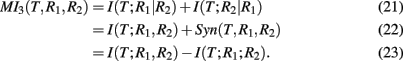
Equation (25) is the sum of two conditional mutual informations between the target gene and a regulator given the other regulator, which emphasizes the three-way nature of this measure. Interestingly, MI₃ has also a simple relation to synergy, as shown in equation (26). This follows directly from equations (10 and 24).

In the right Figure 5, we show a visualization of MI₃. Here, the shown intersections result from the correspondence of I(T; R₁, R₂) to “d + e + f,” I(T; R₁) to “d + e,” and I(T; R₂) to “e + f.” Subtraction of these terms according to equation (24) results in “d + f.” Note that I(T; R₁, R₂) is counted twice.

The MI3 algorithm learns gene regulatory networks in two steps: first, local regulatory networks consisting of only three genes (T, R₁, and R₂) are learned. Starting from a given gene, T, two regulator genes are searched which maximize MI3 (T, R₁, R₂). As a result, directed edges between R₁ and T and R₂ and T are added constituting a small regulatory network. Second, the local regulatory networks learned in step one are assembled. To ensure that the resulting network is acyclic, there may be a need to remove edges forming cycles in the assembled network. This is solved heuristically, by identifying all local three-gene networks that contribute to a cycle and elimination of all edges of them from the overall network, except from the one with the highest MI₃ value. Overall, the MI3 algorithm aims to learn the optimal two-parent causal model for each target variable in the form R1 → T and R2 → T.

CMI (conditional mutual information). Soranzo et al. (2007) use only the conditional mutual information (CMI) to infer regulatory networks. They estimate all conditional mutual information values I(X_i; X_j | X_k) between triplets of genes. Starting from a fully connected network, they successively remove edges A_ij = A_ji = 0 if I(X_i; X_j | X_k) = 0 for at least one gene X_k, according to a threshold condition.

MI-CMI. The MI-CMI algorithm (Liang and Wang, 2008) uses both mutual information and conditional mutual information to estimate the network. Starting from a fully unconnected network G, the algorithm consists of three steps. First, all pairs of mutual information values I(X_i; X_j) are estimated. If I(X_i; X_j) ≥ I₀, then an edge is included, A_ij = A_ji = 1. Second, for all triplets (X_i, X_j, X_k) with I(X_i; X_j) ≥ I₀, I(X_i; X_k) ≥ I₀, and I(X_j; X_k) ≥ I₀ the conditional mutual information for all combinations of I(X_i, X_j, X_k) is estimated. Then based on heuristic rules, is it decided which edges in G are likely to result from indirect regulations (interactions). These edges will be removed from G. Third, for all triplets (X_i, X_j, X_k) with I(X_i; X_j) < I₀, I(X_i; X_k) < I₀, and I(X_j; X_k) < I₀ the conditional mutual information for all combinations of (X_i; X_j; X_k) is estimated. Again, following some heuristic rules, edges that are likely the result from interactive regulations, which could not be detected by mutual information, are included in G. Special emphasize was given to the used statistical estimators, for the mutual information and conditional mutual information values.

Mutual information in combination with conditional mutual information was also used in Zhao et al. (2008), Zhang et al. (2011). However, in contrast to (Liang and Wang, 2008), these approaches are conceptually closer to the PC algorithm (Spirtes et al., 1993; Shipley, 2000).

2.3. Categorization from a Dynamical Perspective

In Figure 6 we present an overview of inference methods to infer regulatory networks, as discussed in the previous section. We separated these methods in two main groups, depending on if the method is correlation- (pink) or information-based (orange). Within these two groups, there are various ways for further subdivision, however, we just distinguish between basic forms and higher order extensions – as indicated by darker colors (see Figure 6).

FIGURE 6

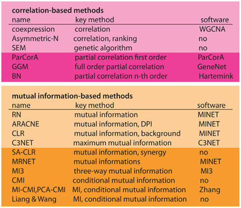
Figure 6. Overview of inference methods to reconstruct regulatory networks from expression data. First column, name of the method. Second column, methodological base of the method. Third column, name of the software package, if available. Horizontal classification, first panel, linear methods (correlation-based). Second panel, non-linear methods (information-based). Darker colors represent extended methods.

2.4. Multiple Testing Corrections

Due to the fact that all methods presented above involve many hypotheses that are tested, one needs to apply a multiple hypothesis correction method (Lehmann and Romano, 2005; Dudoit and van der Laan, 2007). From the investigation of multiple testing corrections it is known that the presence of a correlation structure in the data can lead to severe problems that counteracts an efficient control of an error measure, e.g., of the false discovery rate (FDR) or the family-wise error (Benjamini and Yekutieli, 2001; Storey and Tibshirani, 2003; Dudoit et al., 2008). Unfortunately, in the specific context of the inference of regulatory networks, multiple testing corrections have not been studied well. For this reason, without conducting in depth investigations of this problem one should apply a conservative rather than a more liberal correction method. Hence, one can apply a Bonferroni correction (Bonferroni, 1936; Dudoit and van der Laan, 2007).

3. Evaluation measures

In order to assess the performance of inference methods several measures have been suggested. In the following, we present three different types of such measures: (1) General statistical measures, (2) Ontology-based measures, (3) Network-based measures. On overview of these different measures is given in Figure 7.

FIGURE 7

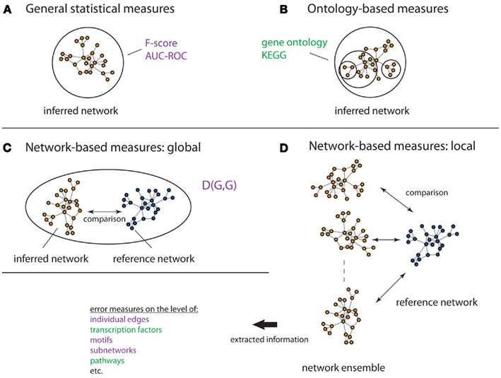
Figure 7. Overview of different evaluation measures. Here, a circle/oval represents the entity that is assessed by a measure, which can be seen as its resolution. The figure visualizes general statistical measures (A), ontology-based measures (B), global network-based measures (C) and local network-based measures (D). The lack of any circle/oval in (D) shall indicate that there is no restriction to any particular resolution level. The measures in green incorporate biological information, whereas the measures in purple do not.

3.1. General Statistical Measures

The most widely used statistical measures are based on,

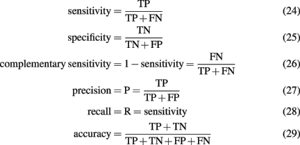
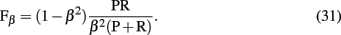
obtained by comparison of a inferred (predicted) network with the true network underlying the data. From the measures listed above, three pair-wise combinations thereof are frequently used to assess the performance of an algorithm. The first measure is the area under the curve for the receiver operator characteristics (AUC-ROC; Fawcett, 2006). The ROC curve represents the sensitivity as function of the complementary specificity obtained by using various threshold values þeta ∈ Θ, instead of one specific, the algorithm depends on³. This leads to a θ-dependence of all quantities listed above and, hence, allows to obtain a functional behavior among these measures. The second measure is the area under the precision-recall curve (AUC-PR), obtained similarly as AUC-ROC, and the third is the F-score,

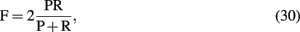
also called F₁ because it is a special form of,

We want to emphasize that all measures presented above are general statistical measures used in statistics and data analysis. None of them is specific to our problem under consideration, namely, the inference of regulatory networks from expression data. In other words, none of these measures utilizes either biological or network specific information in any form. Further, each of these general statistical measures are global error measures because they evaluate the network inference performance as a whole, represented by a scalar value. As a consequence thereof, it is implicitly assumed that the inference process is homogeneous, i.e., each interaction should have about the same true positive rate, because otherwise it would be implausible to summarize the inference performance by just one value, e.g., a F-score. However, this is not justified, as we will discuss below.

In the following, we present extensions of general statistical measures for both types of information.

3.2. Ontology-Based Measures

An evaluation strategy utilizing biological information to assess the performance of an inference method tries to quantify the biological relevance of the inferred network. In general, it is assumed that genes in a gene regulatory network are preferentially linked to genes involved in similar biological processes (Wolfe et al., 2005). There are several publicly available resources of biological knowledge which can be used to test whether this holds true, for example, the Gene Ontology database (GO; Ashburner et al., 2000), or KEGG (Kanehisa and Goto, 2000). There are also several curated organism-specific knowledge databases, such as RegulonDB (E. coli; Gama-Castro et al., 2008) and MIPS (yeast; Mewes et al., 2002). Functional congruence of clusters of coexpressed genes is a popular validation measure for clustering algorithms (Datta and Datta, 2006) and in principle can also be used for the validation of inferred networks.

3.3. Network-Based measures

The third type of measures for assessing the performance of an inference algorithm considers the network structure explicitly. That means, in contrast to the general statistical measures and also the ontology-based measures, network-based measures can only be used if there is a network that underlies the problem.

3.3.1. Global network-based measures

A measure that makes explicit use of the network structures of the true (G) and inferred (Ĝ) network was proposed by Zhao et al. (2008). They suggested to use,

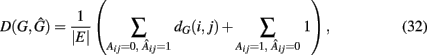
the weighted sum of false-positive edges (first term) plus the false-negative edges (second term). This measure is not only asymmetric in its arguments but also gives a different weight to type-1 (false positives) respectively type-2 (false negatives) errors. For type-1 errors, in the true network G the Dijkstra distance (Dijkstra, 1959) from node i to j, d_G(i,j), is calculated whereas for type-2 errors each false-negative edge is assigned a constant weight of “1.” Overall, D(G,Ĝ) is a global measure, as were all measures discussed in section 1, which assesses the performance of an inference algorithm holistically.

3.3.2. Local network-based measures

In contrast to all above measures, which were global measures, we present finally local network-based measures introduced in Altay and Emmert-Streib (2010b), Emmert-Streib and Altay (2010). These local network-based measures are based on ensemble data, 𝒟 = {D₁(G),…, D_E(G)}, and the availability of a reference network that represents the “true” regulatory network G. Ensemble data means that there is more than one data set available from the biological phenomenon under investigation. This ensemble could be obtained either by bootstrapping from one data set or from simulation studies. The apparent advantage of ensemble data is that they allow to quantify the variability of the population that underlies the data. After having obtained an ensemble of estimated networks yes from 𝒟 = {D₁(G),…, D_E(G)} by application of an inference algorithm, we can obtain the true positive rates ({TPR_ij}) of each edge and the true negative rates ({TNR_ij}) for each non-edge with respect to the underlying true network structure. For example, we can estimate the TPR of an edge between gene i and j, which is present in G, by

which corresponds to Pr(gene i interacts with gene j | 𝒢^e). Analogously, we can estimate the TNR.

Principally, any combination of true positive and true negative rates would result in a valid network-based measure consisting, e.g., of network motifs, subnetworks, or even only of individual edges. For such a measure representing a structural region within a network it is then possible to estimate its reconstruction rate. To provide a concrete example, we give the reconstruction rate of a three-gene motif that is given by the chain in Figure 2

Also, if biological information about the genes in the network is available, this can also be used to define appropriate measures. For example, one could obtain a reconstruction rate for all interactions that are connected with transcription factors or of particular biological pathways involving only certain genes as defined, e.g., via the gene ontology database. Further examples of such measures can be found in Altay and Emmert-Streib (2010b), Emmert-Streib and Altay (2010).

4. Comparison of Inference Methods

A question that is of practical relevance is which of the discussed inference methods, listed in Figure 6, is preferred. Unfortunately, there is no study that compared all these methods with each other. However, there are several studies that compared subsets thereof. For example, in Altay and Emmert-Streib(2010a, 2011) RN, ARACNE, CLR, MRNET, and C3NET have been compared for a large variety of different conditions, including different network structures, sample sizes, and noise levels. For all these conditions, ensemble data have been generated that allow the application of local network-based measures providing the most detailed information about the inference characteristics of a method. Overall, it has been found that C3NET and MRNET perform better than ARACNE, CLR, and RN (in this order). There are two main differences between C3NET and MRNET. First, the computational complexity of C3NET is O(N²) and for MRNET it is between O(N²) and O(N³) which is difficult to quantify exactly because of the iterative nature of the second step employed by MRNET. For the conducted simulations which involved networks in the order of O(10²) genes this was tractable, however, for real biological data the number of genes can reach over 10,000 causing series problems. In contrast, C3NET has been applied to a bootstrap ensemble from B cell lymphoma for 9.684 genes (de Matos Simoes et al., submitted). Second, due to the conservative character of C3NET, which is currently the most conservative method of all inference methods, the number of obtained interactions is easier to deal with than for other methods. For example, in Basso et al. (2005) ARACNE was applied to the same B cell data, inferring about 130,000 interactions whereas C3NET inferred about 10,000 interactions. Given the current impossibility to experimentally validate tens of thousands of interactions by wet lab experiments a conservative subnetwork having a low false-positive rate (Altay and Emmert-Streib, 2010a, 2011) is advantages.

We would like to remark that the methods studied in Altay and Emmert-Streib(2010a, 2011) were selected on the ground of their conceptual similarity to provide a fair comparison, but they have also a (relatively) low computational complexity which allows the investigation for ensemble data and not just single data sets. Many other methods listed in Figure 6 have a higher computational complexity forcing a comparative analysis to be performed with small networks, typically involving O(10¹) genes, and individual data sets rather than ensembles. For example, in Werhli et al. (2006) RN, GGM, and BN have been compared for a network consisting of only 11 genes because of the high computational complexity of a BN. As a result, it is reported that GGM and the BN outperform RN and perform similarly compared to each other.

5. Discussion

From the discussions of the preceding methods for the structural inference of regulatory networks one could get the impression that their number is sheerly unlimited as well as the principle ideas behind them. In our opinion the first point is probably true, the latter not. In order to see this more clearly we would like to outline the general procedure underlying the development of each method. First, a principle idea or hypothesis is raised about a mechanism for the inference of regulatory networks and, second, a method is conceived that could accomplish this. Formally, the first part relates to the conceptual or qualitative framework of a method whereas the latter refers to its quantitative realization, e.g., in form of statistical estimators. In order to learn about two classic inference algorithms, embodying two different conceptual ideas, we presented the IC (inductive causation) algorithm (Pearl, 2000) and the MWST (maximum weight spanning tree) algorithm (Chow and Liu, 1968). For the IC algorithm the conceptual core is d-separation, and for the MWST this is the DPI. When considered from this perspective, the inference algorithms shown in Figure 6 can be grouped as follows. ARACNE is based on the idea of the MWST, whereas all other methods except SEM, SA-CLR, and MI3 are either close or approximate adaptations of d-separation. Here approximate adaptation of d-separation means that an algorithm employs d-separation in a certain way, for instance up to a fixed order of the correlation coefficient or the mutual information (like ParCorA or MI-CMI), but not in the exhaustive way as described for the IC algorithm. From this perspective follow at least three implications. First, the number of conceptually different ideas is very limited if technical approximations are not counted as different. Second, when one of the above inference algorithms represents only an “approximation” of one of the two classic conceptual frameworks its theoretical inference abilities would strictly speaking require a new mathematical proof because new assumptions made may not translate to these methods. Third, due to the fact that most methods presented in Figure 6 lack such a strict mathematical proof our knowledge about their actual abilities is based on numerical studies. This does not mean that numerical studies are not capable of allowing a detailed analysis but that these investigations need to be conducted thoroughly acknowledging the statistical and biological nature of the problem. The former means that numerical studies need to be based on ensemble data in order to capture characteristics of the population, and the latter means that network-based metrics should be applied due to the heterogeneous inferability of local components of regulatory networks, as found in Altay and Emmert-Streib (2010b) and Emmert-Streib and Altay (2010).

We would like to finish this review with a brief outlook on future directions. In the introduction, we mentioned that due to the nature of gene expression data, which do not allow to derive unique predictions about the underlying molecular interactions between gene products, the resulting gene regulatory networks represent a mixture of a transcriptional regulatory network and a protein interaction network. For example, in Altay and Emmert-Streib (2010a) gene expression data from E. coli have been analyzed by inferring a regulatory network. Among the verified interactions found from comparing estimated interactions with experimentally reported results from the literature, transcriptional regulatory interactions, and also protein-protein interactions have been found. Similar results for S. cerevisiae can be found in de Matos Simoes and Emmert-Streib (submitted). In this study, over 800 protein-protein interactions from BioGRID (Breitkreutz et al., 2008) have been identified in the inferred network. For a general discussion about the connection between gene expression and protein interactions, see Grigoriev (2001), Jansen et al. (2002).

In order to obtain more refined predictions about the type of interactions and also to improve the inference performance of the methods, complementary information from other types of high-throughput data is needed. For example, data from ChIP-chip or ChIP-Seq experiments could be used to obtain information about the potential gene targets of transcription factors, similarly, proteomics data could be employed to reveal protein-protein interactions. Ideally, information from all three data types (ChIP-Seq, gene expression, and proteomics) should be integrated to infer a more detailed network with a clearer interpretation of the inferred interactions between the gene products. Sporadically, methods have been already pioneered for such an integration (Nariai et al., 2005; Xing and van der Laan, 2005). However, due to the increased experimental effort and its associated costs the combined availability of several different types of large-scale high-throughput data sets, as necessary for such an analysis, is still rare. This lack of data hampered so far the systematic development of integrative methods. However, with the increasing use of next-generation sequencing technologies this might change is the near future. Other data integration approaches that need to be addressed are the combination of, e.g., gene expression data, from different experiments or platforms (Belcastro et al., 2011). Due to the need for a normalization of such expression data, a pooling of these data is usually prohibitive making an analysis difficult.

Another very important topic, aside data integrative methods, relates to the generation of the data themselves. Specifically, in this review we focused on observational data only, however, experimental data consisting of gene interventions or perturbations form a very fruitful source of information that could be systematically exploited (Fröhlich et al., 2008; Markowetz, 2010; Pinna et al., 2010; Yip et al., 2010).

This discussion emphasizes the need for a clear conceptual distinction between different methods and the information they are based on.

6. Conclusion

In this paper we presented a systematic overview of methods for inferring gene regulatory networks. Although this field is currently vastly expanding making it very difficult to obtain such an overview, we assumed two different perspectives that allowed to categorize inference algorithms sensibly. The first perspective was based on the dynamical assumptions (linear vs. non-linear) methods make about the underlying data. The second considered the methods through the lense of classic approaches which use either d-separation or the DPI (Chow and Liu, 1968; Verma and Pearl, 1991; Spirtes et al., 1993). We want to conclude this article by mentioning that the inference of regulatory networks may not only help in gaining a better understanding of the normal physiology of a cell, but also in elucidating the molecular basis of diseases (Emmert-Streib, 2007; Chen et al., 2008b; Jiang et al., 2008).

Conflict of Interest Statement

The authors declare that the research was conducted in the absence of any commercial or financial relationships that could be construed as a potential conflict of interest.

Acknowledgments

Frank Emmert-Streib would like to thank Simon Tavaré and Florian Markowetz for fruitful discussions and the Department for Employment and Learning through its “Strengthening the all-Island Research Base” initiative and the School of Medicine, Dentistry and Biomedical Sciences for financial support. Gökmen Altay is funded by Cancer Research UK.

Footnotes

^The details of the randomization are different to that used by RN allowing now to make statistical statements.
^We want to remark that I(X; Y; Z) is symmetric in the three variables.
^For example, the mutual information threshold I₀, used in the CLR algorithm.

References

Agrawal, H. (2002). Extreme self-organization in networks constructed from gene expression data. Phys. Rev. Lett. 89, 268702.

Pubmed Abstract | Pubmed Full Text | CrossRef Full Text

Altay, G., and Emmert-Streib, F. (2010a). Inferring the conservative causal core of gene regulatory networks. BMC Syst. Biol. 4, 132.