Flocking to fire: How climate and natural hazards shape human migration across the United States

Introduction

Climate change has already begun to affect life in the United States (US), with temperatures warming by 1.2°F since the 1960s and events like storms and wildfires causing massive disruptions. The US climate is expected to warm by an additional 2.5°F in the next few decades (Hayhoe et al., 2018). As climate change advances, we won't just see warmer average temperatures. We can also expect to see more frequent and severe extreme weather events such as hurricanes, heat waves, and wildfires (Hayhoe et al., 2018; Radeloff et al., 2018). These extreme events can have devastating impacts on people's lives and can influence patterns of human migration (McLeman and Hunter, 2010; Cattaneo et al., 2019).

Each year in the US, natural hazards and disasters in the form of extreme weather events cause numerous deaths and billions of dollars in damages. From 2010 to 2020, hurricanes killed an average of 332 people per year and did an average of $47 billion in damage per year, while wildfires killed an average of 23 people per year and did an average of $7 billion worth of damage per year (NOAA National Centers for Environmental Information, 2022). Heat waves are a leading cause of weather-related deaths in the US. The US Center for Disease Control estimates that heat caused or contributed to an average of 702 deaths per year in the US between 2003 and 2018, counting only official death records (Vaidyanathan et al., 2020); other estimates have been as high as thousands per year (Weinberger et al., 2020).

Some of these impacts are due to a lack of sufficient preparation and planning for natural disasters. For example, Knighton et al. (2021) observed that US cities with strong flood defenses had reduced flood-related deaths and property loss, while cities with poor flood defenses had higher death rates and costlier damage from flooding. Natural disasters have also increased in frequency and scale over time due to population growth in more vulnerable areas (Hunter, 2005). It will be important to consider the spatial relationships between migration and natural hazards as the country invests in strategies for disaster preparedness and climate resilience.

Most of the literature on climate change and natural hazard migration has focused on the Global South (Piguet et al., 2018). Within the US, most such studies have focused on internal migration following specific, punctuating events such as the Dust Bowl of the 1930s or Hurricane Katrina in 2005 (Piguet et al., 2018), or else looked at specific threats such as sea-level rise (e.g., Hauer, 2017). There has been less research on how US migration is affected by natural hazard risk more broadly, or how migration might be affected if climate change amplifies the risk of multiple natural hazards simultaneously. Some recent exceptions include Shumway et al. (2014), and Winkler and Rouleau (2020), which both consider the influence of multiple hazards across longer time periods.

Relationships between migration and the environment—both positive and negative—can be understood using the framework of natural amenity migration. Natural amenities are features of the environment that people value, and that can influence where they choose to live. Natural amenities include factors like a pleasant climate, lakes or ocean, mountains, beautiful scenery, and outdoor recreation (McGranahan, 2008; Lekies et al., 2015; Schaeffer and Dissart, 2018). In the natural amenities framework, natural amenities act as migration “pulls”, attracting new residents or encouraging them to stay, whereas natural hazards (or natural “disamenities”) do just the opposite, acting as migration “pushes” (Hunter, 2005; Shumway et al., 2014; Winkler and Rouleau, 2020).

The idea that people prefer mild climates and varied landscapes—with hills or mountains, lakes or ocean, and a mixture of forest and open space—is supported by the literature on landscape preferences and housing values (McGranahan, 2008; Winkler and Rouleau, 2020). Studies exploring these natural amenities have found significant relationships with migration around the US: in general, people move toward warmer winters, more temperate summers, more varied topography, water bodies, and intermediate levels of forest cover, particularly in rural (nonmetropolitan) areas (McGranahan, 2008; Hjerpe et al., 2020; Winkler and Rouleau, 2020).

The Natural Amenities Scale (McGranahan, 1999) attempts to capture desirable features of the landscape and climate by measuring a suite of natural amenities across the contiguous US: summer and winter temperatures, winter sunshine, summer humidity, topographic variation, water area, and forest cover (with the latter added in McGranahan, 2008). On the Natural Amenities Scale, Florida and the West are rated as rich in natural amenities, while the Midwest and Great Plains rank relatively low. These spatial patterns are closely aligned with long-term migration patterns across the country.

Since the 1950s, 35% of rural counties have seen population declines (Johnson and Lichter, 2019), largely driven by long-term outmigration from rural areas, particularly by the young (Smith et al., 2016). The strongest out-migration has been from rural counties far from metropolitan areas, with few economic opportunities. These areas are concentrated in the Great Plains and along the Mississippi River, regions which are low in natural amenities. In contrast, rural population growth has been strongest in counties near metropolitan areas or high in natural amenities, particularly across the West and along the coasts and mountains of the Southeast (Smith et al., 2016). In recent decades, high-amenity counties have become destinations for recreation and retirement (Smith et al., 2016; Mockrin et al., 2018; Johnson and Lichter, 2019).

Natural amenities can act as a draw for seasonal or permanent migration. This is seen in particular among retirees, for whom income is less tied to place than for working-age adults (Nelson et al., 2009; Lekies et al., 2015; Moeller, 2020). As rural economies have shifted away from manufacturing and extractive industries toward services, many jobs have also become less tied to place (Gosnell and Abrams, 2011; Moeller, 2020). Retirees and teleworkers in particular can choose to live anywhere, and it remains to be seen if the recent rise in telework during the COVID-19 pandemic will lead to a new wave of natural amenity migration.

In addition to natural amenities, socioeconomic factors such as job opportunities, affordability, and population density are also important drivers of migration. Socio-cultural factors such as social networks, cultural norms, crime rates, and family ties also play important roles (Roback, 1982; Czaika and Reinprecht, 2020; Winkler and Rouleau, 2020). Socioeconomic factors can also constrain migration, since the ability to move can be limited by income and access to resources (Hunter, 2005; Cattaneo et al., 2019). Overall, the decision to move is a highly personal one, involving complex tradeoffs among social, economic, and environmental factors.

Existing research on natural amenity migration has identified several literature gaps and areas for continued research, including more interdisciplinary collaborations between social and natural scientists (Gosnell and Abrams, 2011; Lekies et al., 2015; Schaeffer and Dissart, 2018), more use of remote sensing and land cover data (Lekies et al., 2015), and inclusion of natural disamenities (Shumway et al., 2014; Schaeffer and Dissart, 2018), particularly the impacts of climate change and more frequent natural hazards such as fires, floods, and extreme temperatures (Lekies et al., 2015).

We have combined environmental data from a variety of sources to update the Natural Amenities Scale, while also incorporating natural hazards across US counties, alongside a number of socioeconomic covariates. We explore recent US migration patterns (2010–2020) in relation to both natural amenities and disamenities using spatially explicit Spatial Autoregressive (SAR) and Geographically Weighted Regression (GWR) models to address two questions: (1) How do climate, landscape, and extreme weather shape net migration rates across the US? and (2) Are people moving toward or away from the dangers of extreme weather events?

Understanding the baseline relationships between migration and the climate, environment, and extreme weather is an important first step in studying and preparing for migration in response to a changing climate. These relationships might not hold in the long-term, as temperatures and weather events grow more extreme, but they may be our best estimate for the near future. Even if migration patterns suddenly shift, the trends in this study represent not just the transitory movements of people, but also the concomitant decade of investment in housing and infrastructure, which may contribute to lags in any future change in migration patterns.

Our study contributes to the literature by combining spatially explicit biophysical and socioeconomic characteristics into a novel dataset, which we use to rigorously analyze US migration patterns for the most recent decade. According to the literature we have explored, no study has yet examined the most recent national migration trends in relation to natural amenities and natural hazards. To achieve this, our study uses dynamic econometric SAR models and spatially variable GWR models to study both the drivers of migration, and how their relationships with migration vary across space. Our results contribute to a better understanding of migration patterns and provide empirical evidence that can inform strategies for natural hazard planning and preparedness.

Materials and methods

We created a novel dataset from a variety of sources on net migration rates, natural amenities, natural hazards, and socioeconomic factors for each county in the contiguous US (Table 1). Net migration rates, natural hazard frequencies, and socioeconomic drivers were all publicly available as tabular data by US county. In contrast, current US data on natural amenities like climate, water bodies, topographic diversity, and forest cover were only available as raster data, spatially gridded information where each grid cell or pixel contains a value. We overlaid these data with US county boundaries to calculate the county mean or total for each natural amenity variable.

TABLE 1

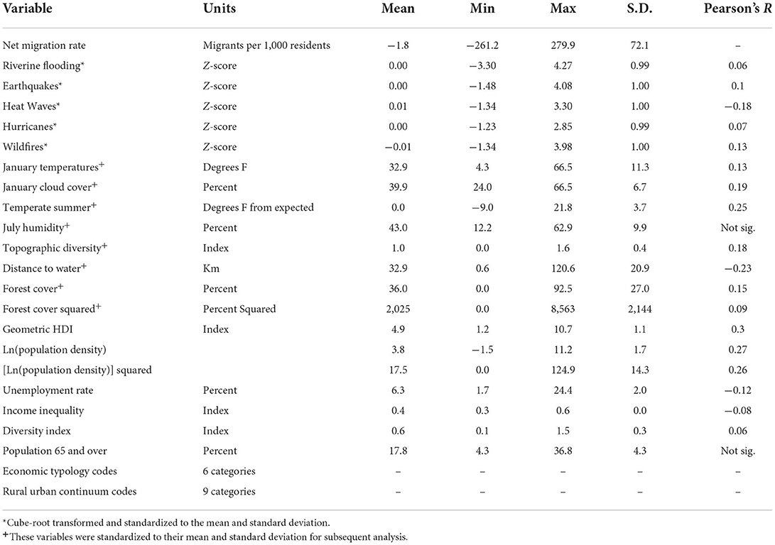
Table 1. Summary statistics and correlations with net migration rates.

In order to investigate the relative importance of different migration drivers, we used the natural amenity, hazard, and socioeconomic variables as covariates in a set of spatially explicit county-level SAR models for net migration, both for the entire contiguous US, and for metropolitan (metro) and nonmetropolitan (nonmetro) counties separately. We also used a subset of these variables as the inputs to a GWR model for net migration in order to map and explore any spatial variations in the relationships between our explanatory variables and migration rates. Our data sources (Supplementary Table 1), processing steps, and analyses are described in the following sections.

Data sets

Net migration rates

We obtained annual county-level population and net migration estimates from the US Census Bureau for the period from 2010 to 2020 (US Census Bureau, 2021d). These county population estimates are for July 1st of each year. Net migration values (population change due to in- and out-migration) are calculated for the period from July 1st of one year to June 30th of the next. To calculate each county's net migration rate for the decade (July 1, 2010–June 30, 2020), we summed each county's annual net migration estimates for this period, normalized by the county's population estimate for July 1, 2010, and scaled to units of migrants per thousand residents (Equation 1).

$\begin{array}{ll}Net& MigrationRat{e}_{2010-2020}=\end{array}$

$\begin{array}{ll}\frac{\sum AnnualNetMigrationEstimates}{PopulationEstimat{e}_{2010}}*1000& (1)\end{array}$

The net migration rates included some extreme outliers. We excluded statistical outliers lying more than three interquartile ranges beyond the first and third quartiles in order to meet statistical assumptions of normality. This excluded 31 of 3,108 counties (< 1%), of which four had large negative values (net outmigration) and 27 had large positive values (net in-migration), leaving 3,077 counties for analysis. The counties with exceptionally high outmigration all had small 2010 population sizes (1,000–35,000 people), meaning an event like the closure of a correctional facility could have an outsized impact. Three of the four negative outlier counties were in or adjacent to migration cold spots (Figure 1), so we feel that regional trends were well represented in the models, even without these outliers. Of the counties with exceptionally high positive values, all but three lay in or near regions characterized by high in-migration such as migration hotspots in Florida, Texas, Utah, North Dakota, and parts of the South (Figure 1). The other three had relatively small initial populations (3,500–66,800). So once again, regional trends are well represented by the surrounding counties, which also experienced high in-migration.

FIGURE 1

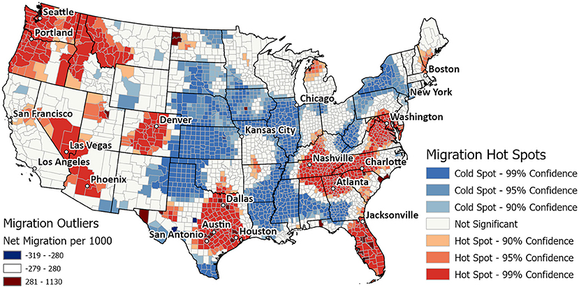
Figure 1. Results of a Getis-Ord Gi* hotspot analysis of county-level net migration rates, 2010–2020. Migration hot spots, where many more people moved into a region than out, are in shades of red. Migration cold spots, where many more people left than arrived, are in shades of blue. Statistical outliers in the net migration data (values lying more than three interquartile distances beyond the interquartile range) were excluded from the analysis, but are shown in the darkest shades of red and blue.

We imported the net migration rates into ESRI's ArcGIS Pro and mapped them using 2020 county boundaries for the contiguous US (US Census Bureau, 2021b). Finally, we created a map of migration hot and cold spots for the last decade using the Getis-Ord Gi^* hot spot statistics (Getis and Ord, 1992; Ord and Getis, 1995) applied through ArcGIS Pro's “Hot Spot Analysis” tool with a Euclidean fixed distance band of 147,000 m (Figure 1).

Natural amenities: Climate variables

Based on the work of McGranahan (1999, 2008), we examined seven natural amenities encompassing climate, surface water, topography, and forest cover. We characterized climate using four variables: January Temperature, January Cloud Cover, July Humidity, and “Temperate Summer”, a measure of relatively mild summer temperatures. Each climate variable is a long-term mean for the period from 1991 to 2020, consistent with the National Oceanic and Atmospheric Administration's (NOAA) most recent climate normals—used to define a place's current climate. We also tested annual precipitation but excluded it after preliminary analyses showed it was strongly correlated with humidity and cloud cover, with no improvement in predicting net migration rates.

We obtained spatially explicit temperature and humidity data for the contiguous US from the GRIDMET dataset hosted on the Google Earth Engine (GEE) Data Catalog (Abatzoglou, 2012). We filtered and processed these data using the GEE API (Gorelick et al., 2017). Daily minimum and maximum temperatures were averaged to calculate separate 30-year means for January and July temperatures. Since January and July temperatures are highly correlated, we calculated a Temperate Summer metric as the negative residual of July Temperatures regressed on January Temperatures. Temperate Summer indicates how much hotter or cooler the summer is than might be expected based on winter temperatures. We calculated the 30-year mean for July humidity using GRIDMET's daily minimum relative humidity levels (Abatzoglou, 2012), as relative humidity is generally lowest around midday when people are active, and highest at midnight.

We obtained raster cloud cover data from NOAA's NCEP-DOE Reanalysis 2 dataset (Kanamitsu et al., 2002) through the GEE Data Catalog and API, and used them to calculate a long-term cloud cover mean. Data for 2006 was unavailable, so we calculated a 29-year mean for the 1991–2020 period, excluding 2006. We used noon values, as the most representative time of day for human activity.

Finally, we imported the 2020 US county boundaries into the GEE API and used them to calculate county means for each of the four climate variables by taking the mean of the raster data within each county polygon, using a 4,000 m scale. Each of these variables was subsequently mapped in ArcGIS Pro.

Natural amenities: Landscape variables

Previous studies of natural amenity migration (McGranahan, 1999, 2008) represented surface water using the natural log of a county's total percent water area, capped at a certain area or percentage. That metric is complicated by the fact that counties along the coasts and Great Lakes include very large areas of coastal waters, sometimes accounting for the majority of a county's area. We consider the mean Distance to Water (including water in other counties) to better capture most residents' relationship with surface water. Many people prefer to live relatively close to water bodies such as lakes and oceans (McGranahan, 2008), but it seems reasonable to assume that the average person cares more about whether there is a water body within driving distance than whether there is one in the same county. Net migration rates also had a stronger relationship with Distance to Water than with the natural log of percent water area (Pearson's R = −0.23 vs. 0.17).

To have a comprehensive and detailed representation of US surface waters, we used the European Commission Joint Research Centre's (JRC) Global Surface Water Mapping Layers, v1.3 (Pekel et al., 2016) accessed via the GEE Data Catalog. To isolate permanent water bodies, we selected areas where the dataset's coded ‘seasonality' band was equal to 12, meaning that surface water was present for 12 out of 12 months in the dataset. We calculated the distance to surface water using a Euclidean distance method (with a 300 km radius kernel) in ArcGIS Pro. We overlaid this distance raster with the 2020 county boundaries to calculate the mean Distance to Water for each county.

The literature on landscape preference and amenity migration supports the idea that humans prefer a varied landscape, including varied topography (McGranahan, 2008). While this is a matter of taste, areas with dramatic hills and mountains tend to be more renowned for their stunning scenery than uninterrupted plains. The Natural Amenities Scale (McGranahan, 1999) measured topographic variation using a ranked categorical scale of landform types, ranging from flat plains to high mountains. Rather than relying on a categorical scale, or a simple metric like elevation, we wanted to use a comprehensive, continuous metric of Topographic Diversity. We chose to represent Topographic Diversity using the 1 km resolution Shannon Index of Geomorphological Landforms (SIGL) from the Amatulli et al. (2018) suite of topographic variables.

While the Shannon Index is often used to measure biodiversity, it can be used to measure the diversity of any type of categorical data, including landform classes. It is a useful metric that balances both the number of distinct classes present, and their evenness or relative abundance. A land area that is mostly flat would receive a low SIGL score, even if it included a small patch of every other landform class. Meanwhile, an area that included an even mix of peaks, slopes, valleys, and flats would receive a high score. One potential limitation is that, since this metric is calculated at a 1 km resolution, it may undervalue very large mountains (e.g., in the Rocky Mountains), where a continuous slope might extend over most of a pixel. We calculated our Topographic Diversity variable as the mean SIGL value for each county in the contiguous US using “Zonal Statistics as Table” tool in ArcGIS Pro. Compared to the categorical variable in the Natural Amenities Scale, our metric had a marginally stronger correlation with net migration rates (Pearson's R = 0.18 vs. 0.15).

As a potential alternative to county means, we also calculated county medians for each preceding amenity variable, but these produced nearly identical maps to the means, consistent with our data being normally distributed. The variable with the largest (but still marginal) difference between mean and median was Topographic Diversity, for which a number of counties had a small value for the mean, but a zero for the median. If we imagine a county consisting of 60% flat plains and 40% hills or mountains, the median would be zero, the same as for 100% flat plains, but the mean would be an intermediate value, which is more representative. For these reasons, we chose to use county means throughout.

We calculated percent Forest Cover for each county in the contiguous US using data from the National Land Cover Database's (NLCD) 2011 Land Cover raster (Yang et al., 2018). NLCD data is available every 2–3 years. We used the 2011 NLCD data as the nearest to the start of the migration period of interest, 2010–2020. We summarized the county area in each of 17 land cover classes and combined the four forest classes (deciduous, evergreen, and mixed forest, and woody wetlands) to represent total percent Forest Cover for each county. Previous research has found a quadratic relationship between forest cover and migration rates (McGranahan, 2008); people prefer a mixed landscape with intermediate forest cover, neither fully wooded nor fully devoid of trees. For this reason, we used both percent Forest Cover and its square as covariates in our net migration models. Net migration was expected to show a positive relationship with Forest Cover and a negative relationship with its square.

We converted each natural amenity variable to a Z-score for subsequent analysis. Each one was also mapped in ArcGIS Pro (Figure 2; Supplementary material).

FIGURE 2

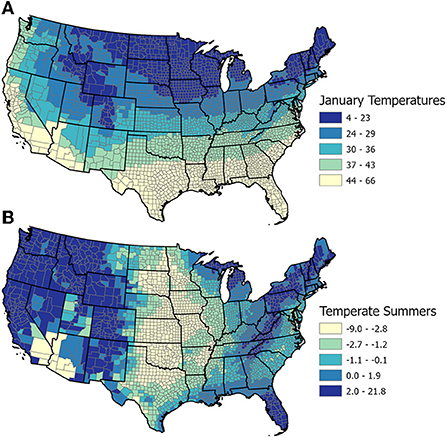
Figure 2. (A) Mean january temperatures in degrees fahrenheit, 1991–2020 (Abatzoglou, 2012). Colder winters are in deeper shades of blue, while the warmest winters are in white. (B) Temperate summers (the negative residual of July over january temperatures), 1991–2020 (calculated from Abatzoglou, 2012). Areas in deeper shades of blue have relatively cooler summers, while those in pale blue and white have relatively hot summers. Counties are grouped and color-coded in quintiles.

Natural hazards data

In order to represent the relative likelihood of experiencing a particular natural hazard in a given county, we obtained the annualized frequencies of 18 different natural hazards from the US Federal Emergency Management Agency's (FEMA) National Risk Index (FEMA., 2020). Of these hazards, we excluded four (avalanches, coastal flooding, tsunamis, and volcanoes) that were missing or inapplicable for more than 30% of counties. For the remaining hazards, we applied a cubed-root transformation to meet assumptions of normality but had to exclude a fifth hazard (landslides) for which the transformation was insufficient.

We assessed the relationships among the remaining hazards and between the hazards and natural amenities using Pearson's correlation coefficients. We used these to select a subset of hazards that minimized multicollinearity while prioritizing the most salient hazards for human health, property damage, and the types of extreme weather expected to be exacerbated by climate change. An example of high multicollinearity would be the high incidence of drought and wildfire in the same counties—these variables often vary together in a consistent and predictable pattern.

Our selected natural hazards included earthquakes, heat waves, hurricanes, riverine flooding, and wildfires. The underlying data for earthquakes and wildfires were modeled probabilities from 2017 to 2016, respectively, while those for riverine flooding, heat waves, and hurricanes were based on the number of recorded events over a period of record: 2005–2017 for heat waves, 1851–2017 for hurricanes, and 1995–2016 for riverine flooding. We converted each natural hazard variable to a Z-score for subsequent analysis. Each one was also mapped in ArcGIS Pro. Maps for hurricanes, heat waves, and wildfires are shown in Figure 3, while earthquakes and riverine flooding are not shown.

FIGURE 3

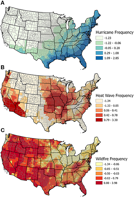
Figure 3. Z-scores of (A) hurricane frequency, (B) heat wave frequency, and (C) wildfire probability (FEMA., 2020). Counties are grouped and color-coded in quintiles.

Socioeconomic data

Socioeconomic factors are major drivers of migration. The most influential socioeconomic factors include job opportunities, cost of living, population density, social services, crime rates, and socio-cultural factors such as social networks, cultural norms, and gender relations (Roback, 1982; Altschul et al., 2020; Czaika and Reinprecht, 2020). Demographics are also important to consider since migration patterns vary across age groups and across race and ethnicity (Johnson et al., 2013; Winkler and Johnson, 2017).

We aimed to control for as many socioeconomic factors as possible, although multicollinearity among certain variables and a lack of data availability for others limited the inclusion of some of these factors in our models. In order to minimize duplicate information between correlated variables, we used the variance inflation factor (VIF) to determine the level of multicollinearity among our entire suite of variables. Any variable that exhibited a VIF >10 was dropped (Hair et al., 2012).

Our final suite of variables is listed in Table 1, and data sources are summarized in Supplementary Table 1. The socioeconomic covariates include: the geometric Human Development Index (HDI), Population Density and its square, the Unemployment Rate, the Gini coefficient of Income Inequality, a Diversity Index of race and ethnicity, the percent of the Population 65 and Over, Economic Typology Codes, and Rural Urban Continuum Codes (RUCC).

The geometric HDI is the geometric mean of three welfare indicators: health (life expectancy at birth), education (the weighted sum of educational attainment and enrollment), and income (per capita personal income). Health, education, and income are strongly related—people with higher incomes tend to have higher education levels and live longer. Since these health, education, and income indicators are highly correlated (Pearson's R correlation coefficients of 0.57–0.63), they cannot be included separately in the models, but by combining them into an index, we are able to incorporate information about all three factors. This index improves on using income alone by adding metrics of health and education outcomes, which themselves reflect a location's underlying health and education infrastructure, such as schools, hospitals, and their quality. The geometric HDI is calculated as follows (Lewis, 2021):

$\begin{array}{l}HDI=\sqrt[3]{health*education*income}(2.1)\\ \text{Where}:education=(\frac{2}{3}attainment+\frac{1}{3}enrollment)\end{array}$

Each welfare indicator is first scaled to an index on a scale of 10 using its minimum and maximum:

$\begin{array}{l}WelfareInde{x}_i=\frac{X_i-X_{imin}}{X_{imax}-X_{imin}}*10(2.2)\end{array}$

X_i = value of welfare indicator i

i = health, attainment, enrollment, income

X_imin = minimum value of X_i

X_imax = maximum value of X_i

We calculated the natural log of Population Density and its square from population and area data from the US Census Bureau. We obtained data on county Unemployment Rates from the US Bureau of Labor Statistics (2022) and took the mean of annual values from 2010 to 2019. The Unemployment Rate accounts for willingness to work by quantifying the number of unemployed active job-seekers in the civilian population over 16 years of age, giving the percentage of this population that are looking for work but have not yet found a position. It is expected to have a negative relationship with net migration rates since people tend to move away from high unemployment (Roback, 1982).

The literature also suggests that crime rates can affect migration (Roback, 1982). While comprehensive county-level data on crime rates is difficult to find, areas with high income inequality tend to have high crime rates (Becker, 1982). Therefore, to indirectly account for crime and other social repercussions of inequality, we include the Gini coefficient, which is a measure of Income Inequality. The Gini coefficient is given by:

$\begin{array}{l}G=\frac{A}{A+B}(3)\end{array}$

where A and B are, respectively, the areas above and below the Lorenz Curve, which measures income distribution. We obtained county-level Gini coefficients from the American Community Survey through the US Census Bureau (2021a). We averaged values from two 5-year periods to calculate means for the period of 2011–2020.

We also included a measure of diversity across race and ethnicity, which has been shown to be a factor in migration dynamics (Nelson et al., 2009; Winkler and Johnson, 2017). We calculated our Diversity Index using the Shannon Index, a useful diversity metric that balances the number of groups and their prevalence in the population. It is calculated as follows:

$\begin{array}{l}H=-{\displaystyle \sum _{i=1}^n}{p}_{i}ln{p}_i(4)\end{array}$

Where p_i is the proportion of the population belonging to each race and ethnicity. For p_i we used the fractions of the population in each of seven racial and ethnic groups, which were calculated as 2010–2019 means using data from the US Census Bureau (2021c). The seven categories were as follows: Non-Hispanic White, Non-Hispanic Black, Non-Hispanic American Indian and Native Alaskan, Non-Hispanic Asian, Non-Hispanic Native Hawaiian and Other Pacific Islander, Hispanic (all races), and Other. The first five categories consisted of individuals who identified as that race alone, while people in the Hispanic category could be of any race. Non-Hispanic individuals who identified as another race or multiracial were included in the Other category, which was calculated as the total population minus the sum of the other six categories.

Age demographics are another important factor influencing migration (Johnson et al., 2013; Frey, 2019). Migration patterns can differ greatly across age groups, and retirees are a particularly important demographic driving in-migration to suburbs and high amenity rural areas. Once retirees are freed from the geographic ties of a job, many choose to move to scenic rural areas, or move closer to adult children. Retirees can also affect migration by attracting younger workers to retirement destinations to work in associated health and assisted living service sectors (Slavov, 2006; Zaiceva, 2014). To better account for these patterns, we have included the percent of each county's Population 65 and Over, calculated as the 2010–2019 mean using demographic data from the US Census Bureau (2021c).

We obtained the Economic Typology Codes, which classify counties by major industries of employment, and the RUCC codes, from the US Department of Agriculture's Economic Research Service (USDA Economic Research Service, 2013, 2015). The Economic Typology Codes classify counties into six mutually exclusive categories, based on counties' principal economic sectors. The categories are defined using the share of a county's earnings or working population employed in the sector. The USDA Economic Research Service (ERS) defines the six economic types as follows:

1. Farming (≥25% earnings or ≥16% employees).

2. Mining (≥13% earnings or ≥8% employees).

3. Manufacturing (≥23% earnings or ≥16% employees).

4. Federal/state government (≥14% earnings or ≥9% employees).

5. Recreation. In addition to employment and earnings, seasonal housing is used to classify recreational counties. The three criteria are given weights and converted to z-scores. The respective weight of each criterion are: 0.3 (earnings), 0.3 (employment) and 0.4 (seasonal housing). A county is regarded as recreational if its index score is ≥0.67.

6. Non-specialized. A county is classified as non-specialized if it is does not fall into any of the five groups listed above.

The RUCC codes classify metropolitan and nonmetropolitan counties into nine categories based on population size, degree of urbanization, and adjacency to a metro area. The RUCC has three metro and six nonmetro categories. The USDA ERS defines the nine RUCC classes as follows (USDA Economic Research Service, 2013):

1. Metro area with one million population or more.

2. Metro area with 250,000 to 1 million population.

3. Metro area of fewer than 250,000 population.

4. Urban population of 20,000 or more, adjacent to a metro area.

5. Urban population of 20,000 or more, not adjacent to a metro area.

6. Urban population of 2,500–19,999, adjacent to a metro area.

7. Urban population of 2,500–19,999, not adjacent to a metro area.

8. Completely rural or < 2,500 urban population, adjacent to a metro area.

9. Completely rural or < 2,500 urban population, not adjacent to a metro area.

We also used the RUCC codes to label each county as either metro (RUCC codes 1–3) or nonmetro (RUCC codes 4–9).

In joining the socioeconomic variables to our other data, we were forced to drop 11 counties that were each missing one or two socioeconomic values, leaving a total of 3,066 counties in our combined dataset.

Analysis and models of net migration rates

We calculated summary statistics for each explanatory variable including the mean, minimum, maximum, and standard deviation (SD) (Table 1). We also calculated the Pearson's R correlation coefficient between each explanatory variable and the net migration rates (Table 1). We further explored the relationships between these explanatory variables and net migration using a series of Spatial Autoregressive Models and a Geographically Weighted Regression model, described in the following sections.

While an ordinary least squares linear regression (OLS) would have been the most straightforward type of model to use, it is not the best model for data that exhibit spatial autocorrelation. Spatial autocorrelation is the tendency for observations that are closer together in space to also have more similar values, a property that is characteristic of most geographic data, including our net migration rates and our environmental and socioeconomic variables. Since neighboring counties often exhibit similar characteristics and similar net migration rates, it is worth considering whether they influence each other through neighborhood effects. For instance, if a given county is high in natural amenities and experiences high in-migration, these factors could influence neighboring counties to also experience high in-migration as people move to be close to a desirable area. A Moran's test for spatial dependence showed that our dataset exhibited strongly significant spatial autocorrelation (Chi² = 1041, p < 0.0001). We therefore chose to use Spatial Autoregressive (SAR) models rather than OLS, since SAR models control for these neighborhood effects.

One limitation of global models like OLS and SAR is that they do not allow for spatial nonstationarity. That is, if there tends to be a positive relationship in one area of the country and a negative relationship in another area, these models will only give a summary of the overall global relationship, masking any spatial variations. We have therefor conducted a Geographically Weighted Regression (GWR), which allows us to map and explore spatial variations in the relationships between net migration and our various drivers.

Spatial autoregressive models

We used SAR models to model the influence of our various environmental and socioeconomic drivers on net migration rates, both globally, and separately for metro and nonmetro counties. It has long been established that there is a neighborhood effect in many spatial data: that societies in one location influence societies in adjacent areas (Durlauf, 2004). We chose to use SAR models rather than OLS in order to account for this neighborhood effect—the impact the covariates and errors of one location have on their neighbors. SAR models account for:

i Spatial lag outcome (L.y)—i.e., an outcome (y) in one given location has an effect on the outcomes in neighboring areas (neighborhood effect—denoted by L, or lag).

ii Spatial lag covariate (L.x)—i.e., a covariate in one location affects the covariates of neighboring locations.

iii Spatially autoregressive errors—i.e., errors in one location affect the errors of neighboring locations.

The SAR model is specified as follows:

$\begin{array}{l}y={\beta }_0+{\beta }_1{W}_{ij}y+{\beta }_{2}x+{\beta }_3{W}_{ij}x+{(I-\phi W_{ij})}^{-1}\epsilon (5)\end{array}$

Where y = the outcome of interest; W_ij = spatial weighting matrix of area i of j-order neighbor, j = 1, 2, … J. The weighting matrix measures the spillover of y or x on neighboring locations. The spillover of y or x on adjacent neighbors is the first-order neighbor and the spillover of areas adjacent to the adjacent areas are the second-order neighbor. The jth neighbor order run from j = 1, 2, … J. If there is no spillover of y or x, then W = 0. The stronger the spillover the greater the value of W. Similarly, the spatially autoregressive error is denoted by φW_ij and has the same jth neighborhood order.

The statistical significance of the jth neighbor order was tested to ensure that all statistically significant indirect impacts were captured and reported.

Model coefficients for SAR models differ from those for linear regression models; because of the extra terms in the SAR model equation, the model coefficients do not correspond to a slope or rate of change as with linear regression models. The model output gives a separate estimate of the direct, indirect, and total $\frac{dy}{dx}$ for each input variable. The direct $\frac{dy}{dx}$ represents the direct effect without considering spatial lags from neighboring counties, while the indirect $\frac{dy}{dx}$considers only the neighborhood spillover effects, and the total is their sum. The direct and indirect effects showed similar trends throughout, so we focus our discussion on the total effects (Table 2).

TABLE 2

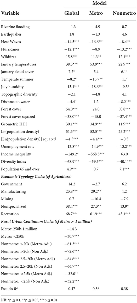
Table 2. Total $\frac{dy}{dx}$ effects for each SAR model.

We ran three separate SAR models: a global model for all counties in our dataset (n = 3,066), a model for nonmetro counties (n = 1934), and a model for metro counties (n = 1,132).

Geographically weighted regression

We used a subset of the socioeconomic, natural amenity, and natural hazard variables to construct a GWR model for Net Migration in ArcGIS Pro, using a fixed distance band of 564,000 m. The GWR constructs a local regression model for each county, using the data for all counties within 564,000 m of that county. Because the GWR consists of a separate model for each county, it allows us to map and explore how the adjusted R² values and model coefficients vary across the country. This allows us to determine if there are regions where the model performs better or worse, and even whether net migration has opposite relationships with a given driver in different parts of the country.

Since the GWR uses spatial subsets of counties, it is highly sensitive to local multicollinearity. That is, if any two input variables exhibit similar spatial clustering, they might be highly correlated within a localized region even if they aren't in the global model. For this reason, we were unable to include all the explanatory variables used in the SAR models. Of the socioeconomic variables, we excluded the RUCC and Economic Typology codes of each county. We were able to include all of the natural amenity variables, but only one of the natural hazard variables: Wildfires. The variables used in each of our four models (three SAR models and one GWR) are summarized in Table 3.

TABLE 3

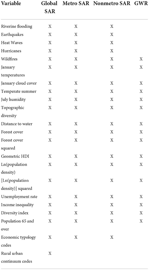
Table 3. Summary of variables used in each model.

Results

Hot spot analysis of net migration rates

Figure 1 shows the Gi^* hot spots for net migration rates across the contiguous US over the last decade (2010–2020). In shades of red are statistically significant migration hot spots, areas where more people have been moving in than out. These can be seen across large areas of the South—particularly around major cities like Nashville, Charlotte, and Atlanta—and across most of Florida, a large portion of Texas, and many areas across the West. In shades of blue are migration cold spots, where more people have been moving out than in. These can be seen across much of the Great Plains and along the Mississippi River, as well as over large portions of New York State and West Virginia.

Natural hazard maps

Hurricanes are mostly an issue along the East and Gulf Coasts of the US, affecting areas from Texas up to Maine (Figure 3A). They more commonly affect coastal areas but can have devastating effects even hundreds of miles inland, such as in land-locked Vermont, which was hit with disastrous flooding in the wake of Hurricane Irene in 2011 (Crossett and Clark, 2021).

Heat waves affect areas along the East and West Coasts, as well as the middle of the country, across the Great Plains and along the Mississippi River (Figure 3B). They are less common in mountainous areas. It is useful to note that heat waves are defined relative to the average temperatures for a given area (FEMA., 2021). In states across the South and Southwest, residents are used to relatively high temperatures, and many are equipped with air conditioning. As a result, it takes much higher temperatures to merit a heat advisory in Texas or Arizona than in Washington State or Maine, where residents are adapted to cold, but may not have air conditioning.

Wildfires affect large swaths of the country, particularly across the West (Figure 3C) where smoke and evacuations have become a routine fact of life in many areas, claiming headlines every summer. However, they also affect counties in the East, where residents may be less aware of this potential danger (Rott et al., 2021).

Summary statistics and correlations with net migration rates

We present the Pearson's R correlation coefficients between net migration rates and each of the natural and socioeconomic variables in Table 1, along with summary statistics for each variable. Net migration rates for counties in the contiguous US (excluding outliers) ranged from −261 to 280 migrants per 1,000 residents, with a mean of −1.8.

The five natural hazards were scaled to their means and standard deviations, so their means were forced to 0.0 and their ranges were compressed to about −1.5–4.1 (−3.3–4.3 for Riverine Flooding). Four of the five hazards had significant positive correlations with net migration (R = 0.06, 0.1, 0.07, and 0.13 for Riverine Flooding, Earthquakes, Hurricanes, and Wildfires, respectively), indicating increased population gains from migration in areas at higher risk of these hazards. However, Heat Waves were significantly and negatively correlated with migration (R = −0.18), suggesting that people have migrated away from this particular hazard.

January Temperatures ranged from 4 to 67°F with a mean of 33°F and were positively correlated with migration rates (R = 0.13), indicating an overall trend of migration toward warmer winters. Temperate Summer (the negative residual of July over January temperatures) values ranged from −9 to 22. Since this is a metric of relative coolness, these can be interpreted as ranging from 9° warmer than expected (given January temperatures) to 22° cooler than expected, with a mean of 0 (the expected temperature in our linear model). Relatively cool, temperate summers were positively correlated with net migration rates (R = 0.25), suggesting an overall trend of moving toward relatively cool summers. January Cloud Cover ranged from 24 to 67% with a mean of 40% and was positively correlated with net migration (R = 0.19), indicating migration toward cloudier areas. July Humidity ranged from 12 to 63% with a mean of 43% and had no significant correlation with migration rates.

Topographic Diversity ranged from 0 to 1.6, with a mean of 1.0, and was positively correlated with migration (R = 0.18), suggesting overall migration toward more topographically diverse landscapes. Distance to water ranged from 0.6 to 121 km, with a mean of 33 km. It was negatively correlated with net migration rates—that is, being a greater distance from water is correlated with lower migration rates (R = −0.23), so areas closer to water would have higher net migration. Forest cover ranged from 0 to 93%, with a mean of 36%. It and its square were both positively correlated with net migration (R = 0.15 and 0.09, respectively), indicating increased net migration with greater forest cover.

The geometric HDI had a mean of 4.9 and was positively correlated with net migration rates (R = 0.3). The natural log of Population Density ranged from −1.5 to 11.2 with a mean of 3.8. This corresponds to raw population densities ranging from 0.22 to 73,130 people per square mile, and a mean of 44.7 people per square mile. The natural log of Population Density and its square were both positively correlated with net migration (R = 0.27 and 0.26, respectively), indicating that people tend to move to more densely populated areas. The Unemployment Rate is the percentage of unemployed active job-seekers in the civilian population over 16 years of age. It ranged from 1.7 to 24.4 with a mean of 6.3 and was negatively correlated with net migration rates (R = −0.12), suggesting migration away from high unemployment rates. Income Inequality (the Gini coefficient) ranged from 0.3 to 0.6 with a mean of 0.4, and was negatively correlated with net migration (R = −0.08). The Diversity Index ranged from 0.1 to 1.5 with a mean of 0.6, and was positively correlated with net migration (R = 0.06). The Population 65 and Over ranged from 4.3 to 36.8 with a mean of 17.8, and had no significant correlation with net migration rates.

Spatial autoregressive models

The SAR results are reported in in Table 2, which shows the total $\frac{dy}{dx}$ effects for the global, nonmetro, and metro SAR models. The direct and indirect effects, model coefficients, and errors are included in the Supplementary Tables 2, 3.

In the global model there was no significant effect for Riverine Flooding or Earthquakes. Both Heat Waves ($\frac{dy}{dx}$ = −14.5) and Hurricanes ($\frac{dy}{dx}$ = −12.1) had negative relationship with net migration as expected. Contrary to expectation however, Wildfires ($\frac{dy}{dx}$ = 15.8) had a positive relationship with net migration. The results for the metro and nonmetro models followed the same trends, although the relationship with Hurricanes was not significant in the metro SAR model (Table 2).

Among the climate variables, summer and winter temperatures were the most important. The global model showed that January Temperatures had a positive relationship with net migration rates ($\frac{dy}{dx}$ = 38.5), indicating that, holding all else equal, people have been moving toward warmer winters. However, Temperate Summers had a negative relationship with net migration rates ($\frac{dy}{dx}$ = −8.2)—that is, controlling for other factors, people have been moving away from areas with cooler, more temperate summers and toward areas with relatively hot summers. This is in contrast to the overall trends captured by the correlation coefficient between Temperate Summers and net migration, which was positive (R = 0.25), suggesting overall migration toward relatively cool summers when we don't control for other variables. The relationship with Cloud Cover was positive ($\frac{dy}{dx}$ = 7.2) while that with Humidity was negative ($\frac{dy}{dx}$ = −13.1). These same trends held for the climate variables in the metro and nonmetro models, with the exception of Cloud Cover in the metro model, and the notable exception of Temperate Summers: while there was a strong negative relationship with migration in metro areas ($\frac{dy}{dx}$ = −13.7), there was no significant relationship in nonmetro areas. This suggests that, holding all else equal, people have been moving toward metro areas with relatively hot summers and away from metro areas with relatively cool summers.

The impact of landscape amenities on migration varied depending on whether metro or non-metro areas were considered. The global model results were not significant for Topographic Diversity and were negative for Distance to Water ($\frac{dy}{dx}$ = −4.4), although the latter was only significant in the nonmetro model, and not in the metro model. The global model showed a positive relationship with Forest Cover ($\frac{dy}{dx}$ = 54.0) and a negative relationship with its square ($\frac{dy}{dx}$ = −38.0), reflecting the expected quadratic relationship. In this case, the metro and nonmetro models showed similar trends, although once again, these relationships weren't significant in the metro model.

Among the socioeconomic variables, the global model showed positive relationships with the Geometric HDI ($\frac{dy}{dx}$ = 30.1) and Population 65 and Over ($\frac{dy}{dx}$ = 4.9), and negative relationships with the Unemployment Rate ($\frac{dy}{dx}$ = −13.8), Income Inequality ($\frac{dy}{dx}$ = −149.2), and the Diversity Index ($\frac{dy}{dx}$ = −68.9). These trends also held true for the metro and nonmetro models, except in the case of Population 65 and Over, which was not significant in the metro model, and Income Inequality, which was not significant in the nonmetro model. The natural log of Population Density had a positive relationship with migration ($\frac{dy}{dx}$ = 51.5) while its square had a negative relationship ($\frac{dy}{dx}$ = −4.5), reflecting the expected quadratic relationship. These trends held true for the metro model, although the relationship with the square was not significant in the nonmetro model. Overall, the socioeconomic variables tended to have stronger relationships with migration in the metro SAR model compared to the nonmetro model (Table 2).

Among the Economic Typology classes, relative to the Agriculture class, Recreation, Nonspecialized, and Manufacturing had significant positive relationships with migration, while Government and Mining were not significant. This held true in the global and metro model, but not the nonmetro model, where the Manufacturing relationship was not significant. Among the RUCC categories, relative to large metro areas with populations over 1 million, every other category had a negative relationship with migration, although the relationship with metro counties with populations between 250,000 and 1 million was not significant. RUCC codes were only included in the global model.

Geographically weighted regression

The results of the GWR model allow us to visualize how model performance (in the form of local R² values for each county) and relationships (in the form of local model coefficients for each county) vary across the country. These results, mapped in Figures 4–6, show how relationships between net migration and variables like Wildfire and Temperate Summer vary spatially, and may be positive in some regions but negative in others. While it is possible to create similar maps for each model driver, we chose to focus on the local Wildfire and Temperate Summer coefficients due to their unexpected results in the SAR models. Wildfire was the only natural hazard included in the GWR.

FIGURE 4

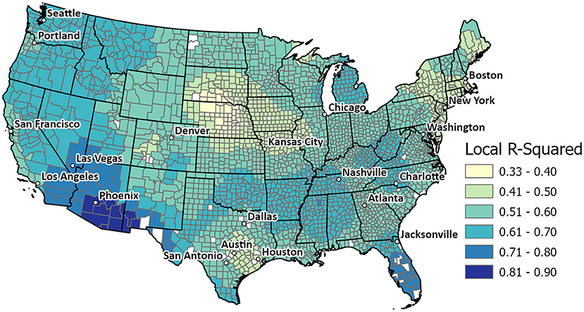
Figure 4. Local R² values for the GWR model. Values ranged from 0.3 to 0.9, with lower values in the Northeast, upper Great Plains and part of Texas, and higher values across the South and West, particularly Arizona and Florida.

FIGURE 5

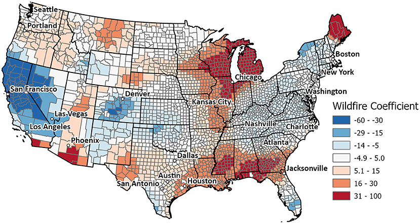
Figure 5. Local model coefficients for wildfire in the GWR. Values ranged from −60 to 100. Negative values (in shades of blue) indicate regions where people have been moving away from counties with a higher risk of wildfires or toward counties with lower risk. Positive values (in shades of red) indicate regions where people are moving toward counties with higher risk or away from counties with lower risk.

FIGURE 6

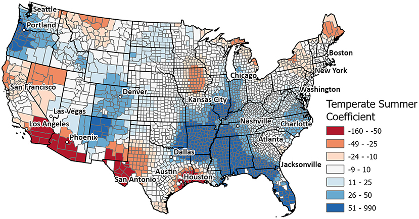
Figure 6. Local model coefficients for temperate summers in the GWR. Values ranged from −160 to 990. Negative values (in shades of red) indicate regions where people have been moving away from counties with relatively cool summers or toward counties with relatively hot summers. Positive values (in shades of blue) indicate regions where people are moving toward counties with relatively cool summers or away from counties with relatively hot summers.

The GWR model had a global adjusted R² of 0.59 and local R² values for each county ranging from 0.3 to 0.9, with lower values in parts of the Great Plains, the Northeast, and Texas, and higher values across the South and West, particularly Arizona and Florida (Figure 4).

Local model coefficients for Wildfire are shown in Figure 5. Values ranged from −60 to 100. Negative coefficients (in shades of blue) indicate regions where people have been moving away from counties with a higher risk of wildfires or toward counties with lower risk. These are seen across much of California and Nevada, in the region around Colorado, New Mexico, Oklahoma, and Kansas, and along the Appalachian Mountains from Tennessee to New Hampshire. Positive values (in shades of red) indicate regions where people are moving toward counties with higher risk or away from counties with lower risk. These are seen in southernmost California, across Arizona and Utah, in the Midwest, Maine, and in states along the Gulf Coast.

Local model coefficients for Temperate Summers are shown in Figure 6. Values ranged from −160 to 990. Negative values (in shades of red) indicate regions where people have been moving away from counties with relatively cool summers or toward counties with relatively hot summers. These can be seen across much of the Southwest and Texas, in Iowa, Montana, and parts of the Northeast. Positive values (in shades of blue) indicate regions where people are moving toward counties with relatively cool summers or away from counties with relatively hot summers. These can be seen across much of the Pacific Northwest, northern Arizona, New Mexico, and Colorado, areas along the Mississippi, and much of the South and Florida.

Discussion

Our study identifies several troubling relationships between US migration patterns and natural hazards. We find that during the 2010s, controlling for environmental and socioeconomic factors, people tended to move away from areas with more frequent heat waves and hurricanes, but toward areas with greater risk of wildfires. In addition, we find that people have been moving toward areas with warmer summer and winter temperatures, including metro areas with particularly hot summers. These trends suggest that migration is increasing the number of people in harm's way, even as climate change continues to exacerbate summer heat and contribute to more frequent and severe wildfires.

We also investigated the relationship of migration to natural amenities and socioeconomic factors. When it came to natural amenities, we found that across nonmetro areas people have generally moved toward cloudier areas, away from higher humidity, closer to water bodies, and toward intermediate levels of forest cover, while people in metro areas don't seem to be as heavily influenced by these factors. Among socioeconomic variables, we found people moved toward areas with higher human development scores (HDI), away from high unemployment and high income inequality, toward large metro areas and areas with intermediate population density, toward more ethnically homogenous areas, and toward areas with larger populations over age 65. We found that, with the exception of the population over 65, all of these factors had stronger effects across metro counties than across nonmetro counties. This suggests migration across urban and suburban areas is more heavily influenced by economic factors, while the natural landscape plays an elevated role in rural areas. Key findings from the SAR models are summarized in Figure 7.

FIGURE 7

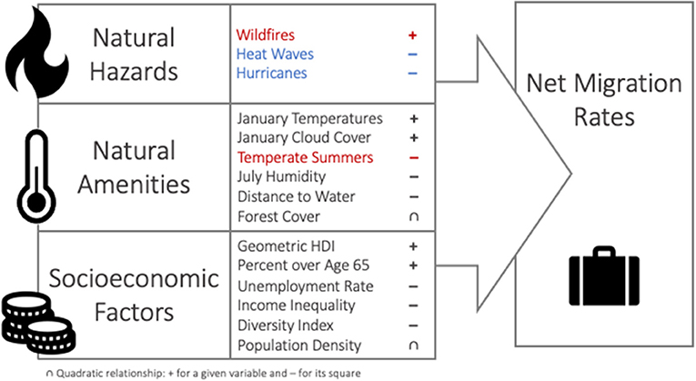
Figure 7. Conceptual diagram highlighting significant relationships between SAR input variables and net migration rates. The most salient relationships given climate change are highlighted in red and blue. Riverine flooding, earthquakes, and topographic diversity were included but not significant. Typologies of major employment sectors and the rural-urban continuum were also included. There were significant positive relationships with manufacturing, recreation, and nonspecialized counties relative to agricultural counties. Relative to large metro counties (population over one million), there were significant negative relationships with RUCC codes designating metro and nonmetro counties of smaller population sizes.

Correlations with net migration

The correlation coefficients with net migration (Table 1) show that, without controlling for any other factors, people have been moving away from areas prone to heat waves, but toward areas at risk of riverine flooding, earthquakes, hurricanes, and wildfires. These results agree with a recent real estate report, which showed that Americans are moving to places with high risks of fire hazards and hurricanes, and that home prices are trending upwards in such places (Katz, 2021).

Among the climate amenities, people moved toward areas with warmer winters and cooler summers. Surprisingly, they also moved toward areas with higher winter cloud cover (R = 0.19). This is in contrast to McGranahan (1999), who found a correlation near zero (R = 0.01) between net migration rates and winter sunshine (1970–1996). This change may be due to our study period seeing very high migration into northwestern states and southern Florida, two regions with particularly cloudy winters. In terms of the landscape amenities, people have been moving toward topographic diversity, closer to water, and toward forest cover. People also moved toward areas with higher HDI values, higher population densities, higher ethnic diversity, lower unemployment rates, and lower income inequalities.

SAR models

Natural hazard and climate variables

While correlation coefficients indicate overall trends in migration relative to each variable, the SAR models represent a given variable's relationship with net migration when we hold all other factors constant, meaning the SAR results are more representative of people's preferences regarding individual variables. The global SAR showed that, after controlling for socioeconomic and environmental factors, people have been moving away from counties most affected by heat waves and hurricanes, but toward those most at risk of wildfires (Table 2). This suggests that people are attracted to fire prone areas. There is a high risk of wildfires across much of the West, as well as parts of the South (Figure 3C), including many areas identified as migration hot spots (Figure 1). It is possible that wildfire-prone areas are representative of the very types of natural scenery and outdoor recreation areas that people find most attractive.

Our results are in line with previous findings of population and housing growth in the fire-prone Wildland Urban Interface (WUI) (Radeloff et al., 2018), and in fire-prone areas more broadly (Bliss et al., 2021; Katz, 2021). Across the US, much of the last decade's population growth and development has taken place in the WUI: suburban and exurban areas in and around forests and wildlands where wildfires are not only more likely, but also harder to fight (Radeloff et al., 2018). The WUI grew by 33% in land area from 1990 to 2020 (Radeloff et al., 2018), and there is evidence that development in this zone—placing more homes, infrastructure, and human activity in fire-prone areas—has led to an increase in human-sparked wildfires (Bar-Massada et al., 2014; Radeloff et al., 2018; Moeller, 2020), which could also contribute to the positive relationship we found between migration rates and wildfires.

This positive relationship is a troubling trend, particularly as climate change is expected to contribute to more frequent wildfires (Radeloff et al., 2018). Our results reflect the complex tradeoffs people must consider as they weigh where to settle. Factors like job opportunities, family ties, affordability, or perceived quality of life could all outweigh the perceived danger of fire.

While natural amenities act as migration “pulls”, disamenities do not always act as “pushes.” People will not relocate if they are not aware of risks, don't take them seriously, or are simply unable to move due to financial or familial constraints. Some will also choose to stay if they accept potential losses as the worthwhile cost of living in a desirable location (Hunter, 2005). Many migrants have been drawn to western states by dramatic mountain scenery and plentiful opportunities for outdoor recreation, but newcomers are often unaware of the potential dangers of wildfires (Bliss et al., 2021), and might not consider the impact of wildfire smoke on day-to-day life. Meanwhile, long-term residents, after repeated exposure to wildfire smoke and evacuations, may become habituated to the danger and no longer consider it as worrisome, a phenomenon documented for other natural hazards (Hunter, 2005). Finally, the poorest residents in at-risk areas may not have the resources to leave, even if they wish to (Hunter, 2005; Cattaneo et al., 2019).

While natural hazards do not always drive local residents to leave, there is some evidence that they can discourage new in-migrants. Hunter (1998) found that US counties with air and water pollution gained fewer new residents than those without. Winkler and Rouleau (2020) found that counties with increased days of extreme heat (days > 90°F) in a given year had suppressed in-migration in the following year. They also found that the occurrence of a FEMA disaster-level wildfire in a given year suppressed net migration in the following year.

At first glance, this appears to contradict our findings of a positive relationship between migration rates and wildfire risk. However, Winkler and Rouleau (2020) only considered the incidence of highly destructive disaster-level fires, while our approach measures wildfire risk more broadly. More importantly, their study focuses on one-year impacts, while ours considers long-term relationships, neither of which fully captures the nuance of how these relationships change over time. Real estate trends suggest that while a wildfire can suppress housing demand in an area for a period of months—when the memory is still fresh in people's minds and burn scars still mar the landscape—these areas often bounce back relatively quickly, seeing rising demand within a few years (Bliss et al., 2021). Affordability may also play an important role—in expensive states where home prices have skyrocketed, homes in the most fire-prone areas can be more affordable, attracting new residents (Bliss et al., 2021; Katz, 2021). It seems that after a few years, when the immediate threat has faded from people's minds, the WUI entices new residents once more.

Heat waves had a strong negative effect on migration in our SAR models, in line with Winkler and Rouleau (2020) findings, and this was stronger in metro areas than in nonmetro areas. This could be due to the urban heat island effect exacerbating hot weather. Compared to more rural or suburban areas, urban areas tend to have less tree canopy, which has cooling and shading effects, and more concrete and other building materials that hold heat (Fokaides et al., 2016).

Despite the negative effect of heat waves, our SAR models show that people preferred to move toward counties with warmer winter temperatures. Somewhat surprisingly, they also preferred to move away from areas with relatively cool, temperate summers and toward those with relatively hot summers. This is in contrast to trends for previous decades when people tended to migrate toward areas with relatively mild summers and winters, such as the Mountain West and California (McGranahan, 1999, 2008). Temperate summers had an even stronger negative effect on migration in metro areas than in the global model—that is, holding all else equal, people moved toward metro areas with relatively hot summers. This could be driven in part by extremely high migration to areas surrounding major cities in Nevada, Arizona and Texas (Figure 1). Meanwhile, temperate summers had no significant effect on migration rates in nonmetro areas.

Our results show that, over the study period, people were attracted to areas with relatively warm summer and winter temperatures, while at the same time avoiding areas prone to heat waves. As air conditioning has become more prevalent, it has enabled more and more population growth in hot climates, such as Arizona, Nevada and Texas. However, as average temperatures continue to warm with climate change, these areas could become more inhospitable. Temperatures could reach a point where they affect residents' health, wellbeing, and quality of life, even with adaptations such as air conditioning (Ebi et al., 2018; Milman, 2018).

Landscape variables

In line with previous literature (McGranahan, 2008; Hjerpe et al., 2020), we found that people preferred to move closer to water, and forest area had a quadratic relationship with migration rates. This is what we would expect, since landscapes with water features tend to be considered more scenic, and the literature suggests that people prefer varied landscapes with intermediate levels of forest cover. These effects were stronger and significant in nonmetro areas, but were non-significant in metro areas. This suggests that pleasant natural scenery plays more of a role in shaping migration patterns in rural areas than in urban ones, where economic opportunities may play a more important role (Winkler and Rouleau, 2020).

Socioeconomic variables

The geometric HDI, an indicator of health, education, and income, had a strong positive effect across the three SAR models, particularly in metro areas. This suggests people are attracted to counties with higher incomes, education levels, and life expectancies, which may be indicative of better economic and educational opportunities, more safety, and higher quality of life. As expected, there was also a strong negative relationship between net migration and unemployment rates. This would be consistent with people being attracted to areas with strong job markets, perhaps even securing employment or other income (such as retirement income) before moving to an area.

We found a very strong positive relationships between income inequality and migration in the global and metro SAR models, but this relationship was not significant in the nonmetro SAR. This is consistent with the idea that income inequality could act as a proxy for crime rates, which may depress net migration rates in urban areas. This relationship does not seem to hold in nonmetro areas, perhaps because rural areas tend to have lower population densities and lower crime rates.

We also found a strong negative relationship in the SAR models between net migration and the Diversity Index, which was in contrast to the positive Pearson's R correlation between these two variables. This indicates that while people have moved toward more diverse areas over all (perhaps as they flock to urban areas), when we control for other factors such as population density and RUCC codes, as we do in the SAR models, we find higher net migration rates in less diverse, generally “whiter” counties. This result is consistent with Winkler and Johnson (2017), who found that black and Hispanic Americans of all ages have been migrating to “whiter” counties (contributing to increased diversity), and older whites of family or retirement age have also been moving to “whiter” counties (decreasing diversity), as they move into suburban or exurban areas. Meanwhile, younger whites have moved toward more diverse urban centers, meaning that overall migration trends, (including people of all races moving toward less diverse, “whiter” areas) have contributed to a national trend of increasing diversity (Winkler and Johnson, 2017; Frey, 2020).

We found a positive relationship between net migration and the population 65 and older in the global and nonmetro SAR models, but this relationship was not significant in the metro SAR. This is consistent with retirement being an important source of in-migration to rural and suburban counties—nonmetro counties with higher populations over age 65 may be retirement destinations that attract new retirees, as well as younger workers who are drawn to jobs in associated service industries. Meanwhile, as retirees become older and less mobile, they are less likely to migrate out again, which also contributes to higher net migration rates.

As expected, population density had a quadratic relationship with migration rates (McGranahan, 2008), indicating that people prefer more densely populated areas up to a point, but dislike excess density, and these effects held true in both the metro and nonmetro models. Controlling for population density and all our other factors, large metro areas with populations over 1 million were generally preferred to other RUCC categories, consistent with the literature's findings of a longstanding rural exodus (Johnson and Lichter, 2019).

Geographically weighted regression

The results of our GWR model can be used to investigate how relationships between net migration and the various environmental and socioeconomic drivers vary across space. Here, we focus on spatial variations in two of the most salient variables for climate change given our SAR results: Wildfires and Temperate Summers.

The relationship between wildfire and net migration varied widely across the country, with positive values in some regions and negative values in others. Figure 5 shows the local model coefficients for the effect of wildfire risk on migration rates. Where counties are red, there is a positive relationship, consistent with our SAR results: people are moving toward wildfire-prone areas (e.g., in the Southwest, Northwest, and Texas) or away from areas less prone to wildfires (e.g., in the Midwest and Maine). Where counties are blue, there is a negative relationship not captured by our SAR model: in these regions people are moving away from wildfire-prone areas (e.g., California) or toward areas less prone to wildfires (e.g., major cities across the South).

The relationship between relatively cool summers and net migration also varies spatially. Figure 6 shows a map of the local model coefficients for the effect of temperate summers on migration rates. Where counties are red, people are moving away from areas with relatively cool summers (e.g., New York, Maine, northern Montana, and northern California), or toward relatively hot summers (e.g., southern California and Arizona). Where counties are blue, people are moving toward areas with relatively cool summers (e.g., the Pacific Northwest, New Mexico, and Colorado) or away from relatively hot summers (e.g., along the Mississippi River).

Limitations and future research

Our results are limited by the variables we did not control for. For instance, housing values, cost of living, and socio-cultural factors, are all important drivers of migration (Czaika and Reinprecht, 2020; Winkler and Rouleau, 2020), but data on these factors were not available at the county level. Socio-cultural factors like professional networks and family ties are particularly hard to measure.

Demographics like age, race, and ethnicity are all important factors influencing migration (Nelson et al., 2009; Johnson et al., 2013; Winkler and Johnson, 2017). Unfortunately, there is no available data for this study period breaking down net migration rates by the age, race, or ethnicity of those moving. Income is also an important factor which often determines who can afford to move. Unfortunately, we are not aware of any county-level data on net migration by income bracket. Our study was only able to control for the static demographic and socioeconomic characteristics of counties, not those of migrants, but there is a need for more research on how recent migration patterns vary across income levels, age, race, and ethnicity, and how these factors interact with each other (Nelson, 2011). It is important to capture both the heterogeneity in people's preferences, and in their ability to act on those preferences, since the option to move to a high-amenity area or avoid environmental disamenities may be highly tied to income and access to resources (Hunter, 2005; Cattaneo et al., 2019).

There is also a role for more research on the social impacts of amenity migration, and its intersection with inequality and environmental justice (Schaeffer and Dissart, 2018). For example, natural amenity migration has the potential to contribute to rural gentrification as relatively wealthy new arrivals buy up property, either for permanent homes, or seasonal second homes. This can drive up the cost of housing, pushing locals to move to more affordable areas (Gosnell and Abrams, 2011). Conversely, some residents of hazard-prone areas may not have the financial means to move out of danger. Research on migration in relation to sea-level rise has identified populations that may become trapped in high-risk areas due to their socio-economic vulnerabilities (Seeteram et al., 2020). Those with lower incomes are generally more vulnerable to natural hazards as they may live in more affordable but higher risk areas, may live in less sturdy housing, and may not be able to afford disaster preparedness or recovery measures like sufficient insurance coverage (Hunter, 2005; Cattaneo et al., 2019).

There is also scope for additional research on the environmental impacts of amenity migration. In some cases, population growth in high-amenity areas, and the associated development, can adversely affect the very environmental factors that attracted migrants in the first place, such as forest wilderness, clean air, clear water bodies, and wildlife (Abrams et al., 2012; Ducey et al., 2016; Mockrin et al., 2018; Radeloff et al., 2018). Much of this new development occurs in the WUI, where people and housing are most at risk from wildfires, and where increased development and human activity has contributed to an increase in human-ignited fires (Radeloff et al., 2018).

Conclusions

Our study analyzes US migration trends for the last decade (2010–2020) in relation to natural amenities and natural hazards. We find that, controlling for socioeconomic and environmental factors, people have been moving toward areas most at risk of wildfire, and toward metropolitan areas with relatively hot summers. As climate change advances, we can expect to see hotter summer temperatures and heightened risk of wildfire, meaning that if these migration trends continue, more and more people will be in danger from heat and fire. We hope our findings will contribute to more awareness of these growing dangers, while providing empirical evidence to guide planners and policymakers as they design strategies for climate resilience and hazard preparedness.

Data availability statement

The original contributions presented in the study are included in the article/Supplementary material, further inquiries can be directed to the corresponding author/s.

Author contributions

MC, EN, and GG conceptualized the paper. MC prepared and visualized datasets and led writing. MC and EN developed methods and conducted formal analysis. EN and GG contributed to analysis, writing, editing, and review. All authors read and approved the final manuscript.

Funding

This work was supported by National Science Foundation Research Traineeship Program (QuEST, Award No. 1735316), USDA Economic Research Service (FAIN 58-6000-2-0066), NASA Socioeconomic Assessment Program (Award No. 80NSSC22K1802), as well as a Pathways Internship at the USDA Economic Research Service, the Gund Institute for Environment and Rubenstein School of Environment and Natural Resources (University of Vermont), and Phil Lasalle/Norman Foundation.

Acknowledgments

We would like to thank David McGranahan, John Cromartie, and John Pender at the USDA Economic Research Service for their early feedback on the project, as well as the attendees of our research seminar. Thank you to committee members Donna Rizzo, Lesley-Ann Dupigny-Giroux, and E. Carol Adair, and thank you to the QuEST Community for their support. We would also like to thank two reviewers who gave very insightful and useful comments, which helped to significantly improve our article.

Conflict of interest

The authors declare that the research was conducted in the absence of any commercial or financial relationships that could be construed as a potential conflict of interest.

Publisher's note

All claims expressed in this article are solely those of the authors and do not necessarily represent those of their affiliated organizations, or those of the publisher, the editors and the reviewers. Any product that may be evaluated in this article, or claim that may be made by its manufacturer, is not guaranteed or endorsed by the publisher.

Author disclaimer

The views expressed are those of the authors and do not necessarily represent those of the USDA.

Supplementary material

The Supplementary Material for this article can be found online at: https://www.frontiersin.org/articles/10.3389/fhumd.2022.886545/full#supplementary-material

References

Abatzoglou, J. T. (2012). Data from: Development of gridded surface meteorological data for ecological applications and modelling. Int. J. Climatol. 27, 2125-2142 doi: 10.1002/joc.3413

CrossRef Full Text | Google Scholar

Abrams, J., Gill, N., Gosnell, H., and Klepeis, P. (2012). Re-creating the rural, reconstructing nature: An international literature review of the environmental implications of amenity migration. Conserv. Soc. 10, 270–284. doi: 10.4103/0972-4923.101837

CrossRef Full Text | Google Scholar

Altschul, J. H., Kintigh, K. W., Aldenderfer, M., Alonzi, E., Armit, I., Barceló, J. A., et al. (2020). Opinion: To understand how migrations affect human securities, look to the past. Proc. Natl. Acad. Sci. 117, 20342–20345. doi: 10.1073/pnas.2015146117

PubMed Abstract | CrossRef Full Text | Google Scholar

Amatulli, G., Domisch, S., Tuanmu, M-. N., Parmentier, B., Ranipeta, A., Malczyk, J., et al. (2018). Data from: A suite of global, cross-scale topographic variables for environmental and biodiversity modeling. Sci. Data 5, 180040. doi: 10.1038/sdata.2018.40

PubMed Abstract | CrossRef Full Text | Google Scholar

Bar-Massada, A., Radeloff, V. C., and Stewart, S. I. (2014). Biotic and abiotic effects of human settlements in the wildland–urban interface. BioScience, 64, 429–437. doi: 10.1093/biosci/biu039

CrossRef Full Text | Google Scholar

Becker, G. (1982). Crime and punishment: an economic approach. J. Pol. Econ. 76, 169–217. doi: 10.1086/259394

CrossRef Full Text | Google Scholar

Bliss, L., Patino, M., and Gu, J. (2021). More Americans Are Moving Into Fire-Risky Areas. Amsterdam, NL: Bloomberg CityLab. Available online at: https://www.bloomberg.com/graphics/2021-moves-into-fire-zones/ (accessed February 01, 2022).

Cattaneo, C., Beine, M., Fröhlich, C. J., Kniveton, D., Martinez-Zarzoso, I., Mastrorillo, M., et al. (2019). Human migration in the era of climate change. Rev. Environ. Econ. Policy 13, 189–206. doi: 10.1093/reep/rez008

CrossRef Full Text | Google Scholar

Crossett, C., and Clark, M. (2021). “Climate change in vermont,” in The Vermont Climate Assessment, eds G. L. Galford, J. Faulkner, J. et al. (2021). Burlington, Vermont: Gund Institute for Environment at the University of Vermont.

Google Scholar

Czaika, M., and Reinprecht, C. (2020). Drivers of migration: A synthesis of knowledge (No. 163; IMI Working Paper Series). Amsterdam: International Migration Institute (IMI).

Google Scholar

Ducey, M., Johnson, K., Belair, E., and Mockrin, M. (2016). Forests in Flux: The Effects of Demographic Change on Forest Cover in New England and New York (National Issue Brief No. 99). Carsey School Public Policy. doi: 10.34051/p/2020.261

CrossRef Full Text | Google Scholar

Durlauf, S. N. (2004). Neighborhood effects. Handbook Reg Urban Econ. 4, 2173–2242. doi: 10.1016/S1574-0080(04)80007-5

CrossRef Full Text | Google Scholar

Ebi, K. L., Balbus, J. M., Luber, G., Bole, A., Crimmins, A., Glass, G., et al. (2018). “Human health,” in Impacts, Risks, and Adaptation in the United States: Fourth National Climate Assessment, Volume II, eds Reidmiller, D.R., C.W. Avery, D.R. Easterling, K.E. Kunkel, K.L.M. Lewis, T.K. Maycock, and B.C. Stewart. (U.S. Global Change Research Program, Washington, DC, USA), 539–571.

FEMA (2020). National Risk Index. Counties Table (NRI_Table_Counties.zip). Available online at: https://hazards.geoplatform.gov/portal/apps/MapSeries/index.html?appid=ddf915a24fb24dc8863eed96bc3345f8 (accessed July 7, 2021).

FEMA (2021). Heat Wave. FEMA National Risk Index. Available online at: https://hazards.fema.gov/nri/heat-wave (accessed February 01, 2022).

Fokaides, P. A., Kylili, A., Nicolaou, L., and Ioannou, B. (2016). The effect of soil sealing on the urban heat island phenomenon. Indoor Built Environ. 25, 1136–1147. doi: 10.1177/1420326X16644495

CrossRef Full Text | Google Scholar

Frey, W. H. (2019). How Migration of Millennials and Seniors has Shifted since the Great Recession. Washington, D.C.: Brookings Institute. Available online at: https://www.brookings.edu/research/how-migration-of-millennials-and-seniors-has-shifted-since-the-great-recession/ (accessed October 28, 2022).

Google Scholar

Frey, W. H. (2020). The Nation is Diversifying Even Faster than Predicted, According to New Census Data. Washington, D.C.: Brookings Institute. Available online at: https://www.brookings.edu/research/new-census-data-shows-the-nation-is-diversifying-even-faster-than-predicted/ (accessed October 28, 2022).

Google Scholar

Getis, A., and J.K. Ord. (1992). The analysis of spatial association by use of distance statistics. Geograph. Anal. 24. doi: 10.1111/j.1538-4632.1992.tb00261.x

CrossRef Full Text | Google Scholar

Gorelick, N., Hancher, M., Dixon, M., Ilyushchenko, S., Thau, D., Moore, R., et al. (2017). Google Earth Engine: Planetary-scale geospatial analysis for everyone. Rem. Sens. Environ. 31, 799–815 doi: 10.1016/j.rse.2017.06.031

CrossRef Full Text | Google Scholar

Gosnell, H., and Abrams, J. (2011). Amenity migration: Diverse conceptualizations of drivers, socioeconomic dimensions, and emerging challenges. GeoJournal 76, 303–322. doi: 10.1007/s10708-009-9295-4

CrossRef Full Text | Google Scholar

Hair, J. F., Sarstedt, M., Ringle, C. M., and Mena, J. A. (2012). An assessment of the use of partial least squares structural equation modeling in marketing research. J. Acad. Market. Sci. 40, 414–433. doi: 10.1007/s11747-011-0261-6

CrossRef Full Text | Google Scholar

Hauer, M. E. (2017). Migration induced by sea-level rise could reshape the US population landscape. Nat. Clim. Change 7, 321–325. doi: 10.1038/nclimate3271

CrossRef Full Text | Google Scholar

Hayhoe, K., Wuebbles, D. J., Easterling, D. R., Fahey, D. W., Doherty, S., Kossin, J. P., et al. (2018). Chapter 2: Our Changing Climate. Impacts, Risks, and Adaptation in the United States: The Fourth National Climate Assessment, Volume II. US: U.S. Global Change Research Program.

Google Scholar

Hjerpe, E., Hussain, A., and Holmes, T. (2020). Amenity migration and public lands: rise of the protected areas. Environ. Manage. 66, 56–71. doi: 10.1007/s00267-020-01293-6

PubMed Abstract | CrossRef Full Text | Google Scholar

Hunter, L. M. (1998). The association between environmental risk and internal migration flows. Popul. Environ. 19, 247–277. doi: 10.1023/A:1024644003699

CrossRef Full Text | Google Scholar

Hunter, L. M. (2005). Migration and environmental hazards. population and environment. Redfin News 26, 273–302. doi: 10.1007/s11111-005-3343-x

PubMed Abstract | CrossRef Full Text | Google Scholar

Johnson, K., and Lichter, D. (2019). Rural Depopulation in a Rapidly Urbanizing America (No. 139; National Issue Brief). Durham, New Hampshire: Carsey School of Public Policy. doi: 10.34051/p/2020.347

CrossRef Full Text | Google Scholar

Johnson, K. M., Winkler, R., and Gers, L. T. R. (2013). Age and Lifecycle Patterns Driving U.S. Migration Shifts (Issue Brief No. 62). Durham, New Hampshire: Carsey Institute.

Google Scholar

Kanamitsu, M., Ebisuzaki, W., Woollen, J., Yang, S., Hnilo, J. J., Fiorino, M., et al. (2002). Data from: NCEP–DOE AMIP-II Reanalysis (R-2). Bull. Am. Meteorol. Soc. 83, 1631–1644. doi: 10.1175/BAMS-83-11-1631

CrossRef Full Text | Google Scholar

Katz, L., and Sandoval-Olascoaga, S. (2021). More People Are Moving In Than Out of Areas Facing High Risk From Climate Change. Available online at: https://www.redfin.com/news/climate-migration-real-estate-2021/

Google Scholar

Knighton, J., Hondula, K., Sharkus, C., Guzman, C., and Elliott, R. (2021). Flood risk behaviors of United States riverine metropolitan areas are driven by local hydrology and shaped by race. Proc. Natl. Acad. Sci. 118. doi: 10.1073/pnas.2016839118

PubMed Abstract | CrossRef Full Text | Google Scholar

Lekies, K. S., Matarrita-Cascante, D., Schewe, R., and Winkler, R. (2015). Amenity migration in the new global economy: current issues and research priorities. Soc. Nat. Resour. 28, 1144–1151. doi: 10.1080/08941920.2015.1054571

CrossRef Full Text | Google Scholar

Lewis, K. (2021). A Portrait of California 2021–2022. New York: Measure of America, Social Science Research Council. Available online at: https://measureofamerica.org/california2021-22/

McGranahan, D. A. (1999). Natural Amenities Drive Rural Population Change (Agricultural Economic Report No. 781). Economic Research Service, U.S. Department of Agriculture.

Google Scholar

McGranahan, D. A. (2008). Landscape influence on recent rural migration in the U.S. Landscape Urban Plann. 85, 228–240. doi: 10.1016/j.landurbplan.2007.12.001

CrossRef Full Text | Google Scholar

McLeman, R. A., and Hunter, L. M. (2010). Migration in the context of vulnerability and adaptation to climate change: Insights from analogues: Migration and adaptation to climate change. Wiley Interdiscip. Rev. Clim. Change 1, 450–461. doi: 10.1002/wcc.51

PubMed Abstract | CrossRef Full Text | Google Scholar

Milman, O. (2018). 'We're moving to higher ground': America's of climate mass migration is here. The Guardian, 4 Available online at: https://www.theguardian.com/environment/2018/sep/24/americas-era-of-climate-mass-migration-is-here (accessed February 01, 2022).

Google Scholar

Mockrin, M. H., Stewart, S. I., Matonis, M. S., Johnson, K. M., Hammer, R. B., Radeloff, V. C., et al. (2018). Sprawling and diverse: The changing U.S. population and implications for public lands in the 21st Century. J. Environ. Manage. 215, 153–165. doi: 10.1016/j.jenvman.2018.03.053

PubMed Abstract | CrossRef Full Text | Google Scholar

Moeller, H-. H. (2020). National Forests are (not) Parks: Managing Amenity Migration to America's National Forests. Cambridge, MA: Massachusetts Institute of Technology.

Google Scholar

Nelson, P. B. (2011). Commentary: special issue of geojournal on amenity migration, exurbia, and emerging rural landscapes. GeoJournal 76, 445–446. doi: 10.1007/s10708-009-9298-1

CrossRef Full Text | Google Scholar

Nelson, P. B., Lee, A. W., and Nelson, L. (2009). Linking baby boomer and Hispanic migration streams into rural America—a multi-scaled approach: Hispanic Migration into Rural America. Popul. Space Place 15, 277–293. doi: 10.1002/psp.520

CrossRef Full Text | Google Scholar

NOAA National Centers for Environmental Information (2022). U.S. Billion-Dollar Weather and Climate Disasters. Available online at: https://www.ncdc.noaa.gov/billions/

Google Scholar

Ord, J. K. A., and Getis. (1995). Local Spatial Autocorrelation Statistics: Distributional Issues and an Application. Geogr. Anal. 27, 286–306. doi: 10.1111/j.1538-4632.1995.tb00912.x

CrossRef Full Text | Google Scholar

Pekel, J. F., Cottam, A., Gorelick, N., and Belward, A. S. (2016). Data from: High-resolution mapping of global surface water and its long-term changes. Nature 540, 418–422. doi: 10.1038/nature20584

PubMed Abstract | CrossRef Full Text | Google Scholar

Piguet, E., Kaenzig, R., and Guélat, J. (2018). The uneven geography of research on “environmental migration.” Popul. Environ. 39, 357–383. doi: 10.1007/s11111-018-0296-4

CrossRef Full Text | Google Scholar

Radeloff, V. C., Helmers, D. P., Kramer, H. A., Mockrin, M. H., Alexandre, P. M., Bar-Massada, A., et al. (2018). Rapid growth of the US wildland-urban interface raises wildfire risk. Proc. Natl. Acad. Sci. 115, 3314–3319. doi: 10.1073/pnas.1718850115

PubMed Abstract | CrossRef Full Text | Google Scholar

Roback, J. (1982). Wages, rents, and the quality of life. J. Pol. Econ. 90, 1257–1278. doi: 10.1086/261120

CrossRef Full Text | Google Scholar

Rott, N., Ropeik, A., and Samuel, M. (2021). United States of Wildfire. Washington, D.C.: NPR. Available online at: https://apps.npr.org/us-wildfires-impact-environment-climate-change/ (accessed February 01, 2022).

Schaeffer, Y., and Dissart, J.-C. (2018). Natural and environmental amenities: a review of definitions, measures and issues. Ecol. Econ. 146, 475–496. doi: 10.1016/j.ecolecon.2017.12.001

CrossRef Full Text | Google Scholar

Seeteram, N. A., Ash, K., Sanders, B., Schubert, J., and Mach, K. J. (2020). Resilience for Whom: A Climate Mobility Framework for Equitable Sea Level Rise Adaptation [Conference presentation). AGU 2020 Fall Meeting, Virtual. Available online at: https://agu.confex.com/agu/fm20/meetingapp.cgi/Paper/674305 (accessed December 09, 2022).

Shumway, J. M., Otterstrom, S., and Glavac, S. (2014). Environmental Hazards as Disamenities: Selective Migration and Income Change in the United States from 2000–2010. Ann. Assoc. Am. Geograp. 104, 280–291. doi: 10.1080/00045608.2013.873322

CrossRef Full Text | Google Scholar

Slavov, N. (2006). Age bias in fiscal policy: Why does the political process favor the elderly? Top. Theor. Econ. 6:1, 1–37. doi: 10.2202/1534-598X.1279

CrossRef Full Text | Google Scholar

Smith, M. N., Winkler, R. L., and Johnson, K. M. (2016). How Migration Impacts Rural America (Brief No. 03–16; Population Trends in Post-Recession Rural America). Madison, Wisconsin: University of Wisconsin-Madison.

Google Scholar

US Census Bureau. (2021a). American Community Survey B19083 Gini Index of Income Inequality. 2015 and 2020: ACS 5-Year Estimates Detailed Tables. Available online at: https://data.census.gov/cedsci/table?q=gini%20indexandg=0100000US%240500000andtid=ACSDT5Y2015.B19083 (accessed September 22, 2022).

US Census Bureau. (2021b). Cartographic Boundary Files 2020. Counties 1:500,000 (shapefile: cb_2020_us_county_500k.zip). Available online at: https://www.census.gov/geographies/mapping-files/time-series/geo/cartographic-boundary.html (accessed July 16, 2021.).

Google Scholar

US Census Bureau. (2021c). County Population by Characteristics: 2010-2019. Annual County Resident Population Estimates by Age, Sex, Race, and Hispanic Origin: April 1, 2010. to July 1, 2019 (CC-EST2019-ALLDATA). Available online at: https://www.census.gov/data/tables/time-series/demo/popest/2010s-counties-detail.html (accessed September 2, 2022).

Google Scholar

US Census Bureau. (2021d). County Population Totals: 2010-2020. Annual Resident Population Estimates, Estimated Components of Resident Population Change, and Rates of the Components of Resident Population Change for States and Counties: April 1, 2010. to July 1, 2020 (CO-EST2020-alldata). Available online at: https://www.census.gov/programs-surveys/popest/technical-documentation/research/evaluation-estimates/2020-evaluation-estimates/2010s-counties-total.html (accessed July 7, 2021).

Google Scholar

US Bureau of Labor Statistics. (2022). Local Area Unemployment Statistics. Labor Force Data by County, 2010-2019 Annual Averages. Available online at: https://www.bls.gov/lau/tables.htm (accessed September 21, 2022).

USDA Economic Research Service (2013). Rural-Urban Continuum Codes. Available online at: https://www.ers.usda.gov/data-products/rural-urban-continuum-codes/

USDA Economic Research Service (2015). ERS County Typology Codes, 2015 Edition. Available online at: https://www.ers.usda.gov/data-products/county-typology-codes/

Google Scholar

Vaidyanathan, A., Malilay, J., Schramm, P., and Saha, S. (2020). Heat-Related Deaths—United States, 2004–2018. MMWR Morb. Mortal. Weekly Rep. 69, 729–734. doi: 10.15585/mmwr.mm6924a1

PubMed Abstract | CrossRef Full Text | Google Scholar

Weinberger, K. R., Harris, D., Spangler, K. R., Zanobetti, A., and Wellenius, G. A. (2020). Estimating the number of excess deaths attributable to heat in 297 United States counties. Environ. Epidemiol. 4, e096. doi: 10.1097/EE9.0000000000000096

PubMed Abstract | CrossRef Full Text | Google Scholar

Winkler, R., and Johnson, K. (2017). Moving to Diversity (Issue Brief No. 117). Durham, New Hampshire: Carsey Institute.

Google Scholar

Winkler, R. L., and Rouleau, M. D. (2020). Amenities or disamenities? Estimating the impacts of extreme heat and wildfire on domestic US migration. Popul. Environ. 42, 622–648 doi: 10.1007/s11111-020-00364-4

CrossRef Full Text | Google Scholar

Yang, L., Jin, S., Danielson, P., Homer, C., Gass, L., Case, A., et al. (2018). Data from: a new generation of the United States National land cover database: requirements, research priorities, design, and implementation strategies. ISPRS J. Photogramm. Rem. Sens. 146,108-123. doi: 10.1016/j.isprsjprs.2018.09.006

CrossRef Full Text | Google Scholar

Zaiceva, A. (2014). The impact of aging on the scale of migration. IZA World of Labor. doi: 10.15185/izawol.99

CrossRef Full Text | Google Scholar