 Andrew Pilny
 Luisa Ruge-Jones2
- 1Department of Communication, University of Kentucky, Lexington, KY, United States
- 2Department of Communication, University of Dayton, Dayton, OH, United States
- 3Department of Communication, University of Illinois Urbana-Champaign, Urbana, IL, United States
Researchers have been increasingly taking advantage of the stochastic actor-oriented modeling framework as a method to analyze the evolution of network ties. Although the framework has proven to be a useful method to model longitudinal network data, it is designed to analyze a sample of one bounded network. For group and team researchers, this can be a significant limitation because such researchers often collect data on more than one team. This paper presents a nontechnical and hands-on introduction for a meta-level technique for stochastic actor-oriented models in RSIENA where researchers can simultaneously analyze network drivers from multiple samples of teams and groups. Moreover, we follow up with a multilevel Bayesian version of the model when it is appropriate. We also provide a framework for researchers to understand what types of research questions and theories could be examined and tested.
Introduction
A network is simply a “set of entities connected by one or more relations” (Contractor and Forbush, 2017; p. 1, emphasis our own). The study of social networks is quite boundary-spanning, significantly evident in social scientific fields like sociology, communication, organizational behavior to more hard scientific fields like computer science and neuroscience. One key aspect network researchers are interested in understanding is why network relations are patterned/structured the way they are. In other words, what influences a network relation to exist in the first place? Theoretically, Borgatti and Halgin (2011) refer to this type of theorizing as theories of networks because they seek to explain why a node will create a network relation with another node (e.g., Monge and Contractor, 2003). For instance, convergence theories like homophily would predict that nodes that share some sort of similarity with one another will be more likely to have a relation in the future than nodes that lack such similarity (e.g., nodes of the similar age).
Essentially, theories of networks seek to find out different network mechanisms responsible for why the network looks the way it does. Stadfeld and Amati (2021) define network mechanisms as the “structural processes that are regularly found in social networks and that can be linked to one or multiple causal social mechanisms of network tie formation” (p. 41, emphasis in original). Generally, there are four domains of network mechanisms: (1) the individual domain, (2) the endogenous domain, (3) the relational domain and (4) the contextual domain (Pilny et al., 2016; Chen et al., 2021). Individual attributes typically refer to either demographic and psychological states of nodes in the network. For instance, are ‘”extraverted” people more likely to form relations in teams? Are their gender differences and inequalities with such relationship formation? Endogenous attributes refer to the idea that certain already-present network structures are responsible for ties looking the way they are. For example, if George creates a tie with Susan at time 1, theories of reciprocity would predict that Susan would create a tie with George at time 2. Relational attributes refer to the presence of other ties as co-evolving with other ties, otherwise known as multiplexity. For instance, theories of activity foci (Feld, 1981) might predict that shared membership with a common focus like their “role” in a team might predict more ties between individuals. Finally, contextual mechanisms are more like “macro” phenomenon and refer to things going on in the environment that influences the entire network. For instance, Wang and Guan (2020) looked at how cultural context influences social media relationships between international government organizations.
Methodologically, usually some type of inferential network model is used to determine if a certain network mechanism is more likely than chance alone. For cross-sectional networks, exponential random graph modeling is a common choice (Lusher et al., 2013). However, for networks with multiple waves, the stochastic actor-oriented modeling (SAOM) framework, first presented by Snijders (1996), is a popular option. Briefly, SAOMs “are a family of models that express empirically observed changes in network ties and in many cases, changes in individual attributes as time-aggregated outcomes of a series of individual decisions” (Kalish, 2020, p. 2)1. These models are “actor-based,” rather than “tie-based” in that the key inference is taken from the perspective of each actor in the network, assuming that they are aware of their environment (i.e., their own ties and attributes of other actors). Between waves of different networks, it is assumed that actors make decisions to change ties in a Markov-like process. The models are estimated by “simulations of sequences of small changes between time-points with parameters adjusted until the simulations can reasonably reproduce the data” (Robins, 2015; p. 195). These sequences are often referred to as ministeps.
Studies using SAOMs have been particularly useful to understand network in organizational and team settings (Chen et al., 2021). However, a key limitation of most applications using SAOMs is that they only apply to one sampled network, albeit in at least more than one wave. For some disciplines like organizational and team research, this can be a significant limitation because such researchers often collect data on more than one sample. For instance, if an organization has ten different teams, it would make sense to collect network from each team rather than just one. Here, there can be a danger of overgeneralization or false inference of network mechanisms from the result of a single network.
The purpose of this paper is to present a nontechnical and hands-on introduction to a meta-level SAOM technique where researchers can simultaneously analyze network drivers from multiple samples of teams and groups (Pasquaretta et al., 2016; e.g., de la Haye et al., 2017). This approach is an aggregation of multiple independent networks into a larger “meta-network” for the purpose of analyzing omnibus effects. We also follow up with a multi-level model using Bayesian inference when assumptions of the meta-network model have been violated. Finally, we also provide a framework to researchers to interpret their results in line with previous research and theory.
Materials and equipment
Before proceeding with the tutorial, we describe the context of the current experiment from which data was collected (Pilny et al., 2014, 2020). The scenario revolved around 8 experimental sessions, consisting of two teams with two people in each team. Participants were 32 undergraduate students from a Midwest university in the United States.
The scenario took place in a video-game simulation called Virtual Battlespace 2 (VBS2; Bohemia Interactive Simulations, 2010). Each of the two teams, in one tank each, started on opposites sites of a city. The key goal was to coordinate their simultaneous arrival to a specific location where they would encounter insurgents and engage in a battle. The teams could only communicate with each other via a radio headset and these messages were logged and recorded. Consistent with each of the three of the four domains of social mechanisms for network tie formation, we gather data on the following:
1. Key network: Trust. Measured from a question reading “To what extent do you trust ___” for each of the other three team members on a Likert scale from 1 = Not at all to 5 = To a very great extent. This variable was dichotomized so that 4 and 5's indicated “trust” and 1, 2, and 3's indicate “not trust”.
2. Individual domain: Gender. Gender was measured as (1) Man, (2) Woman, and (3) Other. Because nobody selected “Other”, it was kept as binary.
3. Relational domain: Communication intensity. A valued matrix was created that indicated the number of messages each person sent during the experimental session. This indicated ‘communication intensity’.
4. Endogenous domain. Reciprocity and closure. These are fairly common endogenous parameters for inferential network models. Because of the small network size (n = 4), we only include these dyadic and triadic configurations.
Methods
What follows is an example code using the eight different groups. We present the following tutorial “from scratch” in order to provide a realistic account for the obstacles that may emerge from conducting such an analysis. Indeed, the following code can be used as a template for specific research projects from a variety of contexts and settings.
Step 1: Install packages
This code simply tells R to find “RSiena” (Ripley et al., 2011) and install it. The second line loads the packages using the ‘library’ function:
install.packages(“RSiena”,,repos =
“http://cran.us.r-project.org”)
library(RSiena)
Step 2: Load key networks
In this example, we have two waves of network trust data from eight groups. For instance, “Group1w1” represents Group #1 from the first wave. The code tells the R to load the data and put it into a list:
netwT1<-list()
netwT1[[1]] <- read.table(“Group1w1.txt”, sep=“ ”)
netwT1[[2]] <- read.table(“Group2w1.txt”, sep=“ ”)
netwT1[[3]] <- read.table(“Group3w1.txt”, sep=“ ”)
netwT1[[4]] <- read.table(“Group4w1.txt”, sep=“ ”)
netwT1[[5]] <- read.table(“Group5w1.txt”, sep=“ ”)
netwT1[[6]] <- read.table(“Group6w1.txt”, sep=“ ”)
netwT1[[7]] <- read.table(“Group7w1.txt”, sep=“ ”)
netwT1[[8]] <- read.table(“Group8w1.txt”, sep=“ ”)
netwT2<-list()
netwT2[[1]] <- read.table(“Group1w2.txt”, sep=“ ”)
netwT2[[2]] <- read.table(“Group2w2.txt”, sep=“ ”)
netwT2[[3]] <- read.table(“Group3w2.txt”, sep=“ ”)
netwT2[[4]] <- read.table(“Group4w2.txt”, sep=“ ”)
netwT2[[5]] <- read.table(“Group5w2.txt”, sep=“ ”)
netwT2[[6]] <- read.table(“Group6w2.txt”, sep=“ ”)
netwT2[[7]] <- read.table(“Group7w2.txt”, sep=“ ”)
netwT2[[8]] <- read.table(“Group8w2.txt”, sep=“ ”)
Once loaded, we will create RSiena objects from them. The important part here is the dimensions. We have four team members in the network and hence, a 4 × 4 matrix. Because we have two waves, the last dimension will be two:
Adv1 <- sienaNet(array(c(as.matrix(netwT1[[1]]), as
.matrix(netwT2[[1]])), dim = c(4, 4, 2)),
allowOnly = FALSE)
Adv2 <- sienaNet(array(c(as.matrix(netwT1[[2]]), as
.matrix(netwT2[[2]])), dim = c(4, 4, 2)),
allowOnly = FALSE)
Adv3 <- sienaNet(array(c(as.matrix(netwT1[[3]]), as
.matrix(netwT2[[3]])), dim = c(4, 4, 2)),
allowOnly = FALSE)
Adv4 <- sienaNet(array(c(as.matrix(netwT1[[4]]), as
.matrix(netwT2[[4]])), dim = c(4, 4, 2)),
allowOnly = FALSE)
Adv5 <- sienaNet(array(c(as.matrix(netwT1[[5]]), as
.matrix(netwT2[[5]])), dim = c(4, 4, 2)),
allowOnly = FALSE)
Adv6 <- sienaNet(array(c(as.matrix(netwT1[[6]]), as
.matrix(netwT2[[6]])), dim = c(4, 4, 2)),
allowOnly = FALSE)
Adv7 <- sienaNet(array(c(as.matrix(netwT1[[7]]), as
.matrix(netwT2[[7]])), dim = c(4, 4, 2)),
allowOnly = FALSE)
Adv8 <- sienaNet(array(c(as.matrix(netwT1[[8]]), as
.matrix(netwT2[[8]])), dim = c(4, 4, 2)),
allowOnly = FALSE)
Step 3: Load attribute data
We will load data from the individual domain (gender) and relational domain (communication intensity). Like Step 2, we will also put them into a list. Once loaded, we need to tell RSiena that this is attribute data using the ‘coCovar’ function for the individual tabular data and “coDyadCovar” for the dyadic attribute in the form of a matrix:
G1=read.table(“Gender_G1.txt”, sep=“ ”)
G2=read.table(“Gender_G2.txt”, sep=“ ”)
G3=read.table(“Gender_G3.txt”, sep=“ ”)
G4=read.table(“Gender_G4.txt”, sep=“ ”)
G5=read.table(“Gender_G5.txt”, sep=“ ”)
G6=read.table(“Gender_G6.txt”, sep=“ ”)
G7=read.table(“Gender_G7.txt”, sep=“ ”)
G8=read.table(“Gender_G8.txt”, sep=“ ”)
Gender<-list()
Gender[[1]] <- G1
Gender[[2]] <- G2
Gender[[3]] <- G3
Gender[[4]] <- G4
Gender[[5]] <- G5
Gender[[6]] <- G6
Gender[[7]] <- G7
Gender[[8]] <- G8
Gender1 <- coCovar(as.matrix(Gender[[1]])[,])
Gender2 <- coCovar(as.matrix(Gender[[2]])[,])
Gender3 <- coCovar(as.matrix(Gender[[3]])[,])
Gender4 <- coCovar(as.matrix(Gender[[4]])[,])
Gender5 <- coCovar(as.matrix(Gender[[5]])[,])
Gender6 <- coCovar(as.matrix(Gender[[6]])[,])
Gender7 <- coCovar(as.matrix(Gender[[7]])[,])
Gender8 <- coCovar(as.matrix(Gender[[8]])[,])
ComIntensiy<-list()
ComIntensiy [[1]]<- as.matrix(read.table(
“Chat_G1.txt”))
ComIntensiy [[2]]<- as.matrix(read.table(
“Chat_G2.txt”))
ComIntensiy [[3]]<- as.matrix(read.table(
“Chat_G3.txt”))
ComIntensiy [[4})@]] (@<- as.matrix(read.table(
“Chat_G4.txt”))
ComIntensiy [[5]]<- as.matrix(read.table(
“Chat_G5.txt”))
ComIntensiy [[6]]<- as.matrix(read.table(
“Chat_G6.txt”))
ComIntensiy [[7]]<- as.matrix(read.table(
“Chat_G7.txt”))
ComIntensiy [[8]]<- as.matrix(read.table(
“Chat_G8.txt”))
ComIntensiy1 <- coDyadCovar(as.matrix(ComIntensiy
[[1]]))
ComIntensiy2 <- coDyadCovar(as.matrix(ComIntensiy
[[2]]))
ComIntensiy3 <- coDyadCovar(as.matrix(ComIntensiy
[[3]]))
ComIntensiy4 <- coDyadCovar(as.matrix(ComIntensiy
[[4]]))
ComIntensiy5 <- coDyadCovar(as.matrix(ComIntensiy
[[5]]))
ComIntensiy6 <- coDyadCovar(as.matrix(ComIntensiy
[[6]]))
ComIntensiy7 <- coDyadCovar(as.matrix(ComIntensiy
[[7]]))
ComIntensiy8 <- coDyadCovar(as.matrix(ComIntensiy
[[8]]))
Step 4: Create meta-network
The next lines of code simply take everything constructed into this point and puts it into a meta-network. The last lines put the networks into an RSiena object:
dataset1 <- sienaDataCreate(Adv = Adv1,
Gender=Gender1, ComIntensity =ComIntensiy1)
dataset2 <- sienaDataCreate(Adv = Adv2,
Gender=Gender2, ComIntensity =ComIntensiy2)
dataset3 <- sienaDataCreate(Adv = Adv3,
Gender=Gender3, ComIntensity =ComIntensiy3)
dataset4 <- sienaDataCreate(Adv = Adv4,
Gender=Gender4, ComIntensity =ComIntensiy4)
dataset5 <- sienaDataCreate(Adv = Adv5,
Gender=Gender5, ComIntensity =ComIntensiy5)
dataset6 <- sienaDataCreate(Adv = Adv6,
Gender=Gender6, ComIntensity =ComIntensiy6)
dataset7 <- sienaDataCreate(Adv = Adv7,
Gender=Gender7, ComIntensity =ComIntensiy7)
dataset8 <- sienaDataCreate(Adv = Adv8,
Gender=Gender8, ComIntensity =ComIntensiy8)
AllGroups <- sienaGroupCreate(list(dataset1,
dataset2, dataset3, dataset4, dataset5,
dataset6, dataset7, dataset8))
GroupEffects <- getEffects(AllGroups) print01Report
(AllGroups, modelname = ’AllGroups’)
A meta-network is simply a collection of different networks into a single network object. In particular, the separate networks are entered into the diagonals of a larger meta-network and the rest of the meta-network is filled with structural zeros (i.e., ties are forbidden). This is a similar procedure one would do with a meta-analysis, combining different studies into a larger meta-dataset to analyze grand effect sizes.
Step 5: Check variability of ties
By looking at the corresponding .txt file from “print01Report,” we need to see if the data is appropriate for analysis, particularly how much the networks overlap with one another. For instance, the Distance column represents the Hamming Distance, which is simply a raw count of how many cells differ from time wave 1 to time wave 2 for each group. However, the Jaccard similarity coefficient may be more useful because it is standardized. A Jaccard coefficient is a measure of overlap between data. For instance, think about how Venn diagram takes two circles and overlaps them to some degree. Imagine circle 1 was time wave 1 and circle 2 was time wave 2. The greater the overlap between the two circles in the Venn diagram, the higher the Jaccard coefficient. Although ideal Jaccard values are a bit subjective, suggested values might range from 0.30 (little overlap: lots of change in ties) to 0.70 (lots of overlap: little change in ties) (Kalish, 2020).
Below, each row represents each group and relevant columns are the possible ties changes and Jaccard coefficient. 0 → 0 simply counts the number of times a tie stayed the same from “no trust” to “no trust. 0 → 1 counts the number of times a tie changed from “no trust” to “trust” and so on. Here, we can see that Group 8 is a significant problem because 1 → 1 represents the amount of times that teams stayed the same from “trust” to “trust,” which is 12 in this case. In other words, Group 8 (i.e., G8) has no variation in changes in trust ties: everybody trusts everybody in both waves:
Tie changes between subsequent observations:
periods 0 => 0 0 => 1 1 => 0
1 => 1 Distance Jaccard Missing
G1: 1 ==> 2 7 2 0 3 2 0.600 0
G2: 3 ==> 4 0 3 0 9 3 0.750 0
G3: 5 ==> 6 3 1 4 4 5 0.444 0
G4: 7 ==> 8 2 3 0 7 3 0.700 0
G5: 9 ==> 10 4 1 1 6 2 0.750 0
G6: 11 ==> 12 3 6 0 3 6 0.333 0
G7: 13 ==> 14 2 6 1 3 7 0.300 0
G8: 15 ==> 16 0 0 0 12 0 1.000 0
As such, let's remove Group 8 because a model cannot possibly try to predict network formation if there is not any present in the data for that group:
CleanGroups <- sienaGroupCreate(list(dataset1,
dataset2, dataset3, dataset4, dataset5,
dataset6, dataset7)) Group_Effects <-
getEffects(CleanGroups) print01Report(
CleanGroups, modelname = ’CleanGroups’)
The remaining seven groups look appropriate to analyze. However, one can make the argument that Groups 2 and 5 should be kept on eye on because of their high Jaccard coefficients (0.75). It is important to remember that these rules of thumbs are somewhat subjective, so with borderline cases, it is up to the researcher to determine which groups might stay and which might go. For instance, if a group with boarderline high/low Jaccard value is preventing a model from run in the first place (i.e., the model does not converge: see Step 6), then this could be a good indicator that removing them would be justified. For now, we just remove Group 8:
Tie changes between subsequent observations:
periods 0 => 0 0 => 1 1 => 0
1 => 1 Distance Jaccard Missing
1 ==> 2 7 2 0 3 2 0.600 0
3 ==> 4 0 3 0 9 3 0.750 0
5 ==> 6 3 1 4 4 5 0.444 0
7 ==> 8 2 3 0 7 3 0.700 0
9 ==> 10 4 1 1 6 2 0.750 0
11 ==> 12 3 6 0 3 6 0.333 0
13 ==> 14 2 6 1 3 7 0.300 0
15 ==> 16 0 0 0 12 0 1.000 0
Step 6: Run and evaluate model
Here we will specify effects for
(1) The individual domain
a. Homophily: Gender (sameX)
(2) The relational domain
a. Multiplexity: Communication intensity (X)
(3) The endogenous domain
a. Density (added by default)
b. Reciprocity (added by default)
c. Closure (transTrip)
Group_Effects <- includeEffects(Group_Effects,
sameX, interaction1
= “Gender”, include=TRUE)
Group_Effects <- includeEffects(Group_Effects, X,
interaction1
= “ComIntensity”, include= TRUE)
Group_Effects <- includeEffects(Group_Effects,
transTrip, include=TRUE)
Group_Model <- sienaAlgorithmCreate(projname
= ’Group_Clean_out’)
Group_Results <- siena07(Group_Model, data
= CleanGroups, effects
= Group_Effects) Group_Results
As a rule of thumb, the convergence t-ratios should ideally be 0, indicating that the simulations are identical to the observed data. In other words, much like a conventional t-test, small t-values represent a failure to reject the null hypothesis of no significant differences between data. Typical cut-off values are 0.10 in absolute value. Likewise, the overall convergence ratio should be less than 0.25 and there may be problems if any parameter has a standard error of greater than 4 (Kalish, 2020).
The first thing reported are rate parameters. These are simply rate values for how many opportunities each actor was afforded to change ties between waves. For instance, in Group 1, each actor was given an opportunity to change their trust ties 0.85 times:
Estimates, standard errors and convergence t-ratios
Estimate Standard Convergence Error t-ratio
Rate parameters:
0.1 Rate parameter period 1 0.8588 ( 0.6207 )
0.2 Rate parameter period 2 2.7922 ( 1.8435
) 0.3 Rate parameter period 3 5.4084 ( 4.2564 )
0.4 Rate parameter period 4 1.4176 ( 0.9073 )
0.5 Rate parameter period 5 0.7423 ( 0.5701 )
0.6 Rate parameter period 6 4.1071 ( 2.5836 )
0.7 Rate parameter period 7 4.5355 ( 2.5470 )
Other parameters:
1. eval outdegree (density) 0.2057 ( 0.8979
)-0.0463
2. eval reciprocity -0.0990 ( 0.8507 ) -0.0648
3. eval transitive triplets 1.0254 ( 0.5130
)-0.0570
4. eval Chistory 0.0522 ( 0.0338 )-0.0561
5. eval same Gender -0.6927 ( 0.7814 )-0.0623
Overall maximum convergence ratio: 0.1066
To get precise probability values to assess statistical significance for hypothesis testing, we can run the following code:
parameter <- Group_Results\$effects\$effectName
estimate <- Group_Results\$theta
st.error <- sqrt(diag(Group_Results\$covtheta))
normal.variate <- estimate/st.error
p.value.2sided <- 2*pnorm(abs(normal.variate),
lower.tail
= FALSE)
(results.table <- data.frame(parameter,estimate
= round(estimate,3),st.error
= round(st.error,3),normal.variate
= round(normal.variate,2),p.value = round(p.
value.2sided,4)))
This returns the following output:
parameter estimate st.error normal.variate p.value
1 outdegree (density) 0.206 0.898 0.23 0.8188
2 reciprocity -0.099 0.851 -0.12 0.9073
3 transitive triplets 1.025 0.513 2.00 0.0456
4 Chistory 0.052 0.034 1.54 0.1226
5 same Gender -0.693 0.781-0.89 0.3753
Here, we can see that there is a significant effect of transitivity (Est. = 1.025, SE = 0.51, p = 0.04). Although it looks like the model converged (i.e., all convergence t-ratios are below 0.10 in absolute vale and overall convergence ratio is below 0.25), we have to check to make sure that the data meets the assumptions of the meta-network model, namely that the effects are the same (i.e., homogenous) across all seven groups.
Step 7: Check for heterogeneity of effects
Indeed, the key assumption of the meta-network approach is that the effects are homogenous across groups, much like we would expect homogeneity of variance across groups in an ANOVA. We can test this using the “sienaTimeTest” function to test this (Lospinoso et al., 2011). The time test essentially creates dummy variables corresponding to the various groups and tests for interactions with the different specified effects following Schweinberger (2012). Here, we will omit the basic density parameter for collinearity reasons:
timetest <- sienaTimeTest(Group_Results, effects
= 2:5) summary(timetest)
Below, we see that the specified effects of reciprocity, transitive triples, communication intensity, and gender homophily are not homogenous across groups given that the p-values are significantly different across the groups:
Effect-wise joint significance tests
(i.e. each effect across all dummies):
chi-sq. df p-value
reciprocity 22.38 6 0.001
transitive triplets 16.85 6 0.010
ComIntensity 26.61 6 0.000
same Gender 32.22 6 0.000
Group-wise joint significance tests
(i.e. each group across all parameters):
chi-sq. df p-value
Group 1 4.75 4 0.314
Group 2 2.09 4 0.719
Group 3 24.98 4 0.000
Group 4 5.38 4 0.250
Group 5 5.21 4 0.266
Group 6 21.98 4 0.000
Group 7 5.28 4 0.260
From the output, one can see that Group 3 (χ2 = 24.98, p < 0.01) and Group 6 (χ2 = 21.98, p < 0.01) are significantly different with respect to their parameter estimates. If your data demonstrates such heterogeneity, there may be serious questions on whether or not the estimates are reliable or not because the assumption of homogeneity has been violated. This suggests that a meta-network model is not exactly appropriate for your data. However, this does not mean that researchers are out of options and need to abandon the SAOM framework because there are available options to account for such heterogeneity of effects described next.
Step 8: Consider a multilevel model
In cases of significant heterogeneity of effects, there are actually three options available: (1) including dummy variables represent different groups, a (2) meta-analysis, and/or (3) a multilevel model using Bayesian estimation. The first option of using dummy variables to account for heterogeneous groups is feasible, but comes at the risk of creating bloated models that may be overfitting the data. For instance, in the current example, if we include dummy variables for the four effects that were heterogeneous, this means including an additional 24 variables [(N groups – 1)×(number of heterogeneous variables)]. Likewise, meta-analysis options sound just like what they are traditionally used for: they run independent models for each group, treat them as essentially independent experiments, and calculate omnibus/aggregate effect sizes for each parameter. However, for small networks (e.g., n < 8), independent models still need to be run. These models will likely return unreliable estimates given the complex Markov Chain Monte Carlo simulations used (see for e.g., Yon et al., 2021) and are thus not appropriate for the current data. Put simply, when small-sized groups are combined into a large meta-network, sample size is not an issue, but by themselves, they will be too small.
However, a multilevel model can be used using Bayesian estimation because it still preserves the larger meta-network. Here, we can specify the current effects as fixed and also allow them to vary randomly (Koskinen and Snijders, 2022). The first step is to install the “RSienaTest” package:
install.packages(“RSienaTest”, repos= “http://R-Forge.R-project.org”)
library(RSienaTest)
Then, specify the effects to be random. For initial guidance on what parameters should be random, the time-test in Step 7 may be a good place to start. As such, we'll start off with all parameters as fixed and random:
Group_Effects2 <-setEffect(Group_Effects, density,
random=TRUE)
Group_Effects2 <-setEffect(Group_Effects2, recip,
random=TRUE)
Group_Effects2 <-setEffect(Group_Effects2,
transTrip, random=TRUE)
Group_Effects2 <-setEffect(Group_Effects2, sameX,
interaction1
= “Gender”, random=TRUE)
Group_Effects2 <-setEffect(Group_Effects2, X,
interaction1
= “ComIntensity”,random=TRUE)
print(Group_Effects2, includeRandoms=TRUE,
dropRates=TRUE)
The multilevel model uses Bayesian estimation. Although a full treatment of Bayesian estimation is beyond the scope of this tutorial (see Koskinen and Snijders, 2022), we will briefly describe it. Bayesian estimation is often contrasted with null hypothesis significance testing (NHST). Bayesian estimation attempts to calculate the probability of a parameter being significant given the observed data, rather than the probability of observing the data given that a parameter is not significant (i.e., assuming the null hypothesis is true). For example, consider the prosecutor's fallacy (see West and Bergstrom, 2020). If your DNA was found at a crime scene, NHST would give you the odds of a false positive, the odds of the observing the data assuming DNA testing technology was incorrect (H0). Although useful, this may not be the most relevant question at hand. For example, in the prosecutor's fallacy, it is very unlikely to observe a false positive in a DNA test and thus, we can reject the null hypothesis (H0) that the DNA test is wrong. On the other hand, Bayesian thinking would give you the odds of the alternative hypothesis (H1) being true, the odds that you are guilty given that you have a DNA match. Here, the number may be pretty low as well, meaning that there are several other folks who have the same DNA profile that matched the crime scene. Put this way, Bayesian tests against H1 rather than H0.
However, Bayesian estimates depend on the probability of the alternative hypothesis (H1) before considering the observed data (i.e., calculating the base rate). In the prosecutor's fallacy, this is easy because we know that only one person committed the crime. In this case, we can estimate what is called a prior, a belief on what the base-rate estimate would be before collecting data. This is contrasted with an uninformed prior, which means that any parameter value can have an equal chance of occurring. Whether or not informed or uninformed priors are specified, a Bayesian model will estimate what are called posterior probabilities, which evaluate the odds of a parameter being significant after considering the data. But of course, posterior probabilities depend on the original priors and corresponding p-values indicate the odds that a parameter is significant given the observed data. Some benefits of Bayesian estimation are that it sample sizes are typically not an issue and it may be asking a more straightforward question to testing hypotheses regarding parameter values. On the other hand, Bayesian estimation is highly influenced by the priors, which should ideally come from previous theory and research.
Koskinen and Snijders (2022) specify priors based on previous research on the evolution of network ties. With respect to density (i.e., outdegree), they specify a value of−1 given that most socially constructed networks between individuals tend to be sparse. On the other hand, they specify reciprocity as +1, given that reciprocity tends to be evident in a variety of social networks. Uninformed priors are used for the remained fixed effects. Finally, sigma values of 0.01 represent the case that groups should tend to be similar to one another via their standard deviations, 10 times smaller than variations within groups.
Mu2 <- rep(0,6)
Mu2[2] <--1 # outdegree
Mu2[3] <- 1 # reciprocity
Sig2 <- matrix(0,6,6
diag(Sig2) <- 0.01
Sig2
#check to see if it worked correctly
(reffs <- Group_Effects2\$shortName[(Group_Effects2
\$include & ((!Group_Effects2\$basicRate &
Group_Effects2\$randomEffects) |(Group_Effects2
\$basicRate & (Group_Effects2\$group$==$1))))])
cbind(reffs, Mu2, sig=diag(Sig2))
Finally, the model can be run. A warning: this estimation might take a while because it is simulating thousands of networks based on different possible estimation values, comparing them to the observed network, and then refining over and over again. The current estimation took about 3 min to run, but will likely be longer for larger networks and more groups:
Group_Results_Bay <- sienaBayes(Group_Model, data
= CleanGroups,initgainGlobal=0.1,
initgainGroupwise = 0.02,effects
= Group_Effects2, priorMu = Mu2, priorSigma
= Sig2,priorKappa =0.01,prevAns
= Group_Results,nwarm=50, nmain=250,
nrunMHBatches=20,nbrNodes=8, silentstart=FALSE
)
The output is reported below. Remember, we are testing the odds that the parameters are significant given the data (i.e., verifying) rather than the probability of observing the data given the null being true (i.e., falsifying), so high p-values indicate significance (i.e., greater than 0.95):
Posterior means and standard deviations are
averages over 1000 MCMC runs (counted after
thinning).
Post. Post. cred. cred. p
mean s.d.m. from to
1. rate constant Adv rate (period 1) 3.1176 (
1.2151 ) 1.2234 5.5436
2. rate constant Adv rate (period 3) 2.7666 (
1.1867 ) 1.0233 5.6828
3. rate constant Adv rate (period 5) 2.9593 (
1.4361 ) 0.8371 6.2014
4. rate constant Adv rate (period 7) 4.6209 (
1.6297 ) 1.6911 8.0913
5. rate constant Adv rate (period 9) 2.9782 (
1.2002 ) 1.0002 5.2208
6. rate constant Adv rate (period 11) 2.2482 (
1.4391 )) 0.4014 5.7365
7. rate constant Adv rate (period 13) 2.9784 (
1.2021 ) 1.0253 5.7258
8. eval outdegree (density) 1.5097 ( 0.5948 )
0.2824 2.6564 1.00
9. eval reciprocity −1.0469 ( 0.6063 )−2.1123
0.1609 0.06
10. eval transitive triplets 0.9941 ( 0.4210 )
0.1462 1.7706 0.99
11. eval ComIntensity 0.2137 ( 0.1184 )−0.0021
0.4563 0.97
12. eval same Gender −0.7570 ( 0.6398 )−1.8731
0.4100 0.12
Post.sd cred.from cred.to
eval outdegree (density) 0.2135 0.0889 0.4183
eval reciprocity 0.2039 0.0917 0.4095
eval transitive triplets 0.2006 0.0887 0.4219
eval ComIntensity 0.2357 0.1099 0.4185
eval same Gender 0.2228 0.0855 0.4877
Step 9: Interpret initial results
Here, we can see that the posterior means for multiplexity (PM = 0.21, p = 0.97) and transitivity (PM = 0.99, p = 0.99) effects remain significant. Moreover, the density parameter is now significant as well (PM = 1.50, p > 0.99).
However, what about the random effects specified below the output? Here, what are returned are posterior between-group standard deviations (SDs). Along with these SDs are credibility intervals that show each SD is quite different than zero. However, we would rarely expect group effects to be exactly the same (i.e., an SD of zero), so these SD estimates do not tell us much about statistical significance. In the next step, we will determine both convergence and if we can relax any of the effects specified as random.
Step 10: Assess convergence
The quickest, but perhaps most subjective way to analyze convergence is by looking at trace and density plots for the fixed and random effects. The Y-axis is the average value and the X-axis represents the point of the MCMC chain. Essentially, an ideal plot is a perfect perpendicular line with the X-axis that demonstrate consistent estimates across the MCMC chain with observations varying randomly across the line. If the line takes a linear or even nonlinear shape, it means that the final Bayesian estimates may be skewed and untrustworthy because they are not consistent across iterations. In the first run, we can see that convergence is unlikely to be evident (see Figure 1):
RateTracePlots(Group_Results_Bay)
NonRateTracePlots(Group_Results_Bay)
In essentially all of the plots, we see that the model has a tough time settling on a consistent value. For example, take a look at the average theta value for reciprocity (in red). It seems to oscillate even between negative and positive throughout all of the simulations. This is an obvious sign that the final posterior mean may not be an accurate estimate given that the model seems confused on whether or not reciprocity is less or more likely in trust formation.
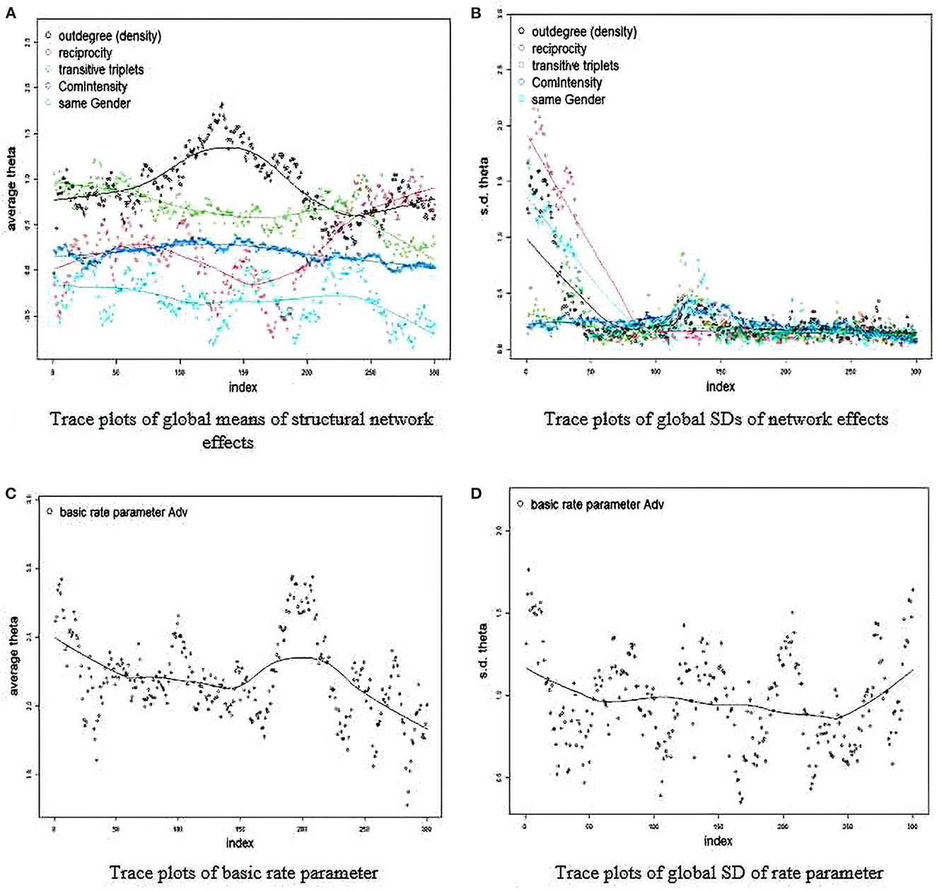
Figure 1. (A–D) Trace plot for convergence diagnosis. Initial estimation (bad convergence). SD, standard deviation; Adv, name of key network; Theta, estimated coefficient; Index, iteration in estimation chain.
More often than not, the first estimate will not be the last and will take efforts to refine and tune a final model. Following the literature and our own personal experiences, below are some tips at fine-tuning a model:
1. Sometimes there are too many random effects specified. We suggest iteratively choosing variables with the highest chi-square values from the “sienaTimeTest” in Step 7.
2. Sometimes successive simulations in generated estimates are too correlated with one another. Increasing the multiplication factor will help reduce the correlation between successive network simulations and thus, increase the amount of Monte Carlo Markov chain steps. This can be done in the creation of the algorithm. The default multiplication factor is 5. Here, we can increase it to 20:
Group_Model_Second_ru <- sienaAlgorithmCreate(
projname = ’Group_Clean_out’, mult =
20)
3. Continue an estimate from previous session using the prevBayes command. If you ‘start from scratch’, it may take a large number of runs to converge on reliable estimates. As such, starting from a previous estimate give the algorithm a better starting off point. For instance:
Group\_Model_Second_run <- sienaBayes(Group_Model,
data = CleanGroups, effects
= Group_Effects2, nmain= 100, nSampConst
= 5, nrunMHBatches = 20, prevBayes
= Group_Model_First_run)
4. Smaller values on “initgainGlobal” (default = 0.1) can improve stability for the initial Moment of Methods estimation for the larger meta-network. Likewise, lower values on “initgainGroupwise” (default=0.02) can help stabilize estimates for the separate groups, which may be even more relevant for small networks (e.g., N < 8). These gain settings determine the step sizes for the parameter updates and thus, small values try to prevent extreme changes in parameter values from iteration to iteration. Moreover, the “reductionFactor” (default = 0.5) controls the multiplier for the observed rate parameter covariance matrix to obtain the prior covariance matrix for the basic rate parameters. Lower values may aid in stabilization, especially if one notices significant divergence later in the chain of simulations. Finally, larger values on “nrunMHBatches” (default = 20) can help too because they increase the number of iterations the algorithm will go through to find reliable estimates (see also “nmain” and “nwarm”). For instance:
Group_Results_Third_run <- sienaBayes(Group_Model,
data = CleanGroups, initgainGlobal=
0.01, initgainGroupwise = 0.001, effects
= Group_Effects2, priorMu = Mu2, priorSigma
= Sig2, priorKappa = 0.01, prevAns
= Group_Results_Second_run, reductionFactor =
0.1, nwarm = 50, nmain= 1000, nrunMHBatches =
50, nbrNodes = 8, silentstart =FALSE)
After several iterations, consistent values could not be found for reciprocity and transitivity. As such, we removed random effects for these parameters and found, for the most part, a stable and converged model. Significant random effects are still evident as well as significant fixed effects for communication (multiplexity) and transitivity, but no longer for density:
Posterior means and standard deviations are
averages over 1000 MCMC runs (counted after
thinning).
Post. Post. cred. cred.
p mean s.d.m. from to
1. rate constant Adv rate (period 1) 2.5196 (
1.1710 ) 0.6761 5.1651
2. rate constant Adv rate (period 3) 3.5734 (
1.3000 ) 1.5524 6.5103
3. rate constant Adv rate (period 5) 2.6259 (
0.9591 ) 1.0805 4.7202
4. rate constant Adv rate (period 7) 2.7331 (
1.0610 )) 1.0245 5.1777
5. rate constant Adv rate (period 9) 1.5176 (
0.7621 ) 0.4086 3.2985
6. rate constant Adv rate (period 11) 2.4509 (
0.8880 ) 1.0834 4.5508
7. rate constant Adv rate (period 13) 2.8393 (
0.8879 ) 1.3907 4.7376
8. eval outdegree (density) 1.0668 ( 0.9912 )
−0.5668 3.2752 0.85
9. eval reciprocity 0.6101 ( 0.9716 ) −2.5576
1.1201 0.28
10. eval transitive triplets 1.1104 ( 0.5592 )
0.2430 2.3519 0.99
11. eval ComIntensity 0.1847 ( 0.1347 ) −0.0424
0.5081 0.95
12. eval same Gender −0.3813 ( 0.7945 ) −1.9397
1.1922 0.29
Post.sd cred.from cred.to
eval outdegree (density) 0.2589 0.0923 0.5912
eval ComIntensity 0.2381 0.1031 0.4641
eval same Gender 0.2094 0.0796 0.4496
Below, the trace plots demonstrating some preliminary evidence of convergence and stability (Figure 2). However, the outdegree parameter could perhaps be more fine-tuned to be bit more stable because it seems to vary up and down along the iterations:
NonRateTracePlots(Group_Results_Third_run)

Figure 2. (A–D) Trace plot for convergence diagnosis. Second estimation (much better, but not acceptable convergence). SD, standard deviation; Adv, name of key network; Theta, estimated coefficient; Index, iteration in estimation chain.
For the effects that were specified as random, it is useful to create density plots along the groups (see Figure 3) to determine how significant they are. However, it is important to note that this is a more qualitative assessment of significance since we do not have exact probability values on what a typical standard deviation would be between groups regarding specified effects:
AllDensityPlots(Group_Results_Third_run, legendpos
= “topright”)
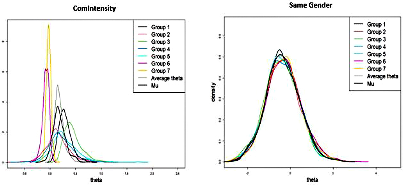
Figure 3. Density plots for random effects. Theta, estimated coefficient, Mu, Observed coefficient.
By visualizing the average thetas across each group, it might be worth specifying Gender as only a fixed effect since the thetas are so similar across groups. For instance, there is considerable overlap with the lines representing each group, which would suggest high levels of homogeneity after controlling for other parameters. On the other hand, multiplexity is well conceptualized as a fixed and random effect give the different distributions across groups. As such, we can run the model with gender homophily as only a fixed effect:
GroupEffects4 <- getEffects(CleanGroups)
GroupEffects4 <- setEffect(GroupEffects4, density)
GroupEffects4 <- setEffect(GroupEffects4, recip)
GroupEffects4 <- setEffect(GroupEffects4, transTrip
)
GroupEffects4 <- setEffect(GroupEffects4, sameX,
interaction1
= “Gender”)
GroupEffects4 <- setEffect(GroupEffects4, X,
interaction1
= “ComIntensity”)
GroupEffects4 <- setEffect(GroupEffects4, density,
random=TRUE) GroupEffects4 <- setEffect(
GroupEffects4, recip, random=FALSE)
GroupEffects4 <- setEffect(GroupEffects4, transTrip
, random=FALSE) GroupEffects4 <- setEffect(
GroupEffects4, sameX, interaction1
= “Gender”, random=FALSE)
GroupEffects4 <- setEffect(GroupEffects4, X,
interaction1
= “ComIntensity”, random$=$TRUE) print(
GroupEffects4, includeRandoms=TRUE,
dropRates=TRUE)
Mu2 <- rep(0,3)
Mu2[2] <--1 # outdegree
Sig2 <- matrix(0,3,3)
diag(Sig2) <- 0.01
Group\_Results\_Model1 <- sienaBayes(Group\_Model,
data
= CleanGroups,initgainGlobal=0.01,
initgainGroupwise = 0.0001,effects
= GroupEffects4, priorMu = Mu2, priorSigma
= Sig2, priorKappa = 0.01,prevAns
= Group\_Results,nwarm=50, nmain=200,
nrunMHBatches=50,nbrNodes=8, silentstart=FALSE
)
Group\_Results\_Model2 <- sienaBayes(Group\_Model,
data
= CleanGroups,initgainGlobal=0.001,
initgainGroupwise = 0.00001,effects
= GroupEffects4, reductionFactor =
.05, nwarm=50, nmain=1000, nSampConst
= 5, nrunMHBatches=100,prevBayes
= Group\_Results\_Model1)
Posterior means and standard deviations are
averages over 1000 MCMC runs (counted after
thinning).
Post. Post. cred. cred. p
mean s.d.m. from to
1. rate constant Adv rate (period 1) 2.6455 (
1.3979 ) 0.5963 5.8551
2. rate constant Adv rate (period 3) 4.2995 (
1.5241 ) 1.6973 7.5919
3. rate constant Adv rate (period 5) 2.8170 (
1.1100 ) 1.0805 5.4946
4. rate constant Adv rate (period 7) 2.8435 (
1.1817 ) 0.9359 5.4299
5. rate constant Adv rate (period 9) 1.4391 (
0.7493 ) 0.3393 3.1714
6. rate constant Adv rate (period 11) 2.6891 (
1.0114 ) 1.1060 5.0570
7. rate constant Adv rate (period 13) 3.2440 (
1.1451 ) 1.4667 5.8413
8. eval outdegree (density) 1.0494 ( 1.2207 )
−0.7532 3.7799 0.81
9. eval reciprocity -0.4934 ( 0.9038 ) −2.3617
1.1128 0.30
10. eval transitive triplets 1.0262 ( 0.4686 )
0.2161 2.1151 1.00
11. eval ComIntensity 0.1730 ( 0.1153 ) -0.0251
0.4269 0.95
12. eval same Gender -0.5202 ( 1.1184 ) -2.9204
1.4767 0.33
Post.sd cred.from cred.to
eval outdegree (density) 0.2506 0.0817 0.5575
eval ComIntensity 0.2111 0.0931 0.4095
The trace plots (Figure 4) look quite better than the previous run with homophily as a random effect. For instance, most of the average thetas and standard deviations are quite stable along the iterations:
RateTracePlots(Group_Results_Model2)
NonRateTracePlots Group_Results_Model2)

Figure 4. (A–D) Trace plot for convergence diagnosis (good convergence). SD, standard deviation; Adv, name of key network; Theta, estimated coefficient; Index, iteration in estimation chain.
Discussion
After producing converged result, it seems reasonable to discuss them in light of previous research and theory. However, given the eclectic nature of studies employing social network analysis, we would encourage researchers to consider similar (1) node and (2) relation types of previous studies. The point here is to avoid making over-generalized statements on the nature of social networks.
For instance, consider our results in the context of similar studies looking at human work team's trust networks. Lusher et al. (2014) looked at a cross-sectional network trust structures of three professional football (i.e., “footy”) teams and found some similar and differing results. Whereas transitivity was evident in most of the teams, reciprocity was also evident. Similarly, Lusher et al. (2012) looked at trust networks within a corporate management team for producing sailboats and motor sails in Italy. They too found evidence of positive transitivity, null reciprocity, and negative gender homophily (the current results has a negative, albeit insignificant parameter). Indeed, the key differences in some of these studies is that the current is a zero-history experimental design, but also the fact that we looked at the evolution of trust rather than a cross-sectional snapshot. As for trust evolutionary dynamics and growth, the current results suggest that trust evolution seems to be more of a triadic (i.e., transitivity), rather than dyadic (i.e., reciprocity) phenomenon.
Finally, although the relationship between communication intensity and trust formation significantly varied across the groups, the final fixed effect was positive. This supports previous work that demonstrates the multiplex nature of trust, that is, trust is rarely a network relation that two nodes might have in isolation from other ties (e.g., Ellwardt et al., 2012; Lusher et al., 2012; Su, 2021). In particular, the current results support a communicative constitution and negotiation of trust, meaning that communication seems to underlie the formation of trust, rather than trust emergence as a simple contagious process (e.g., Schoeneborn et al., 2018). Put simply, the results may suggest that trust in groups seems to be related to group communication somehow, although the relationship could certainly be seen as bi-directional (e.g., two group members now trust each other, so they talk more with each other). Future research may consider the ways multiple network co-evolve with one another.
In sum, the following paper demonstrates some of the questions that could be answered if researchers have multiple samples of longitudinal networks they seek to model. Figure 5 summarizes the steps provided here into a decision-tree format for researchers to use. Using the SAOM framework, we presented a hands-on tutorial on meta-network and multilevel network models that could be appropriate to reveal what network mechanisms may be responsible for why the network evolved the way it did.
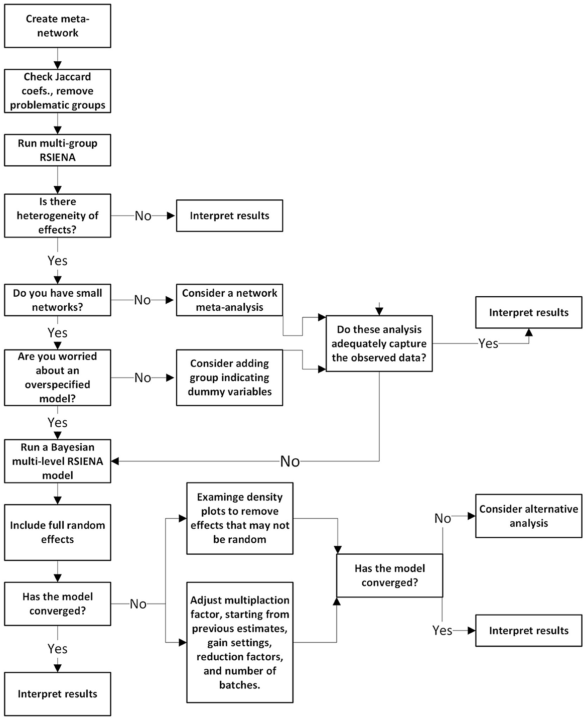
Figure 5. Decision tree format for modeling evolution of network dynamics for multiple groups.
Data availability statement
The original contributions presented in the study can be found in the following OSF link: https://osf.io/6a2z9/?view_only=ef805cb13d294e6f8ac324174588f126.
Ethics statement
The studies involving human participants were reviewed and approved by University of Illinois Institutional Review Board. The patients/participants provided their written informed consent to participate in this study.
Author contributions
AP: writing and data analysis. LR-J and MP: writing. All authors contributed to the article and approved the submitted version.
Funding
The data from this research was sponsored by the Army Research Laboratory (ARL) and was accomplished under Cooperative Agreements W911NF-09-2– 0053 and W5J9CQ-12-C-0017 (the ARL Network Science CTA). The views and conclusions contained in this document are those of the authors and should not be interpreted as representing the official policies, either expressed or implied, of the Army Research Laboratory or the U.S. Government. The U.S. Government is authorized to reproduce and distribute reprints for Government purposes notwithstanding any copyright notation here on.
Conflict of interest
The authors declare that the research was conducted in the absence of any commercial or financial relationships that could be construed as a potential conflict of interest.
Publisher's note
All claims expressed in this article are solely those of the authors and do not necessarily represent those of their affiliated organizations, or those of the publisher, the editors and the reviewers. Any product that may be evaluated in this article, or claim that may be made by its manufacturer, is not guaranteed or endorsed by the publisher.
Footnotes
1. ^The following paper only considers modeling the evolution of network relations, rather than also modeling the evolution of attributes simultaneously (i.e., co-evolutionary models).
References
Bohemia Interactive Simulations. (2010). Virtual Battlespace 2. Bohemia Interactive Simulations. Available online at: http://products.bisimulations.~com/products/vbs2 (accessed June, 2022).
Borgatti, S. P., and Halgin, D. S. (2011). On network theory. Organ. Sci. 22, 1168–1181. doi: 10.1287/orsc.1100.0641
Chen, H., Mehra, A., Tasselli, S., and Borgatti, S. P. (2021). Network dynamics and organizations: a teview and tesearch agenda. J. Manage. 48, 1602–1660. doi: 10.1177/01492063211063218
Contractor, N., and Forbush, E. (2017). “Networks.” in: The International Encyclopedia of Organizational Communication. (Eds.) Scott, C., and Lewis, L. doi: 10.1002/9781118955567.wbieoc148
de la Haye, K., Embree, J., Punkay, M., Espelage, D. L., Tucker, J. S., and Green, H. D. (2017). Analytic strategies for longitudinal networks with missing data. Soc. Networks 50, 17–25. doi: 10.1016/j.socnet.2017.02.001
Ellwardt, L., Wittek, R., and Wielers, R. (2012). Talking about the boss:effects of generalized and interpersonal trust on workplace gossip. Group Org. Manag. 37, 521–549. doi: 10.1177/1059601112450607
Feld, S. L. (1981). The focused organization of social ties. Am. J. Sociol. 86, 1015–1035. doi: 10.1086/227352
Kalish, Y. (2020). Stochastic actor-oriented models for the co-evolution of networks and behavior: an introduction and tutorial. Organ. Res. Methods 23, 511–534. doi: 10.1177/1094428118825300
Koskinen, J., and Snijders, T. A. (2022). Multilevel longitudinal analysis of social networks. arXiv preprint arXiv 2201:12713. Available online at: https://arxiv.org/pdf/2201.12713.pdf
Lospinoso, J. A., Schweinberger, M., Snijders, T. A. B., and Ripley, R. M. (2011). Assessing and accounting for time heterogeneity in stochastic actor oriented models. Adv. Data Anal. Classif. 5, 147–176. doi: 10.1007/s11634-010-0076-1
Lusher, D., Koskinen, J., and Robins, G. (2013). Exponential Random Graph Models for Social Networks. New York, Cambridge University Press. doi: 10.1017/CBO9780511894701
Lusher, D., Kremer, P., and Robins, G. (2014). Cooperative and competitive structures of trust relations in teams. Small Group Res. 45, 3–36. doi: 10.1177/1046496413510362
Lusher, D., Robins, G., Pattison, P. E., and Lomi, A. (2012). “Trust Me”: differences in expressed and perceived trust relations in an organization. Soc. Networks 34, 410–424. doi: 10.1016/j.socnet.2012.01.004
Monge, P., and Contractor, N. (2003). Theories of Communication Networks. Oxford: Oxford University Press. doi: 10.1093/oso/9780195160369.001.0001
Pasquaretta, C., Klenschi, E., Pansanel, J., Battesti, M., Mery, F., and Sueur, C. (2016). Understanding dynamics of information transmission in drosophila melanogaster using a statistical modeling framework for longitudinal network data (the RSiena Package). Front. Psychol. 7, 539. doi: 10.3389/fpsyg.2016.00539
Pilny, A., Dobosh, M., Yahja, A., Poole, M. S., Campbell, A., Ruge-Jones, L., et al. (2020). Team coordination in uncertain environments: the role of processual communication networks. Hum. Commun. Res. 46, 385–411. doi: 10.1093/hcr/hqz020
Pilny, A., Schecter, A., Poole, M. S., and Contractor, N. (2016). An illustration of the relational event model to analyze group interaction processes. Group Dyna. Theory Res. Pract. 79, 376–396. doi: 10.1037/gdn0000042
Pilny, A., Yahja, A., Poole, M. S., and Dobosh, M. A dynamic social network experiment with multi-team systems. Big data cloud computing (BdCloud), (2014). IEEE Fourth International Conference. IEEE. (2014), 587–593. doi: 10.1109/BDCloud.2014.81
Ripley, R. M., Snijders, T. A., Boda, Z., Vörös, A., and Preciado, P. (2011). Manual for RSIENA. Oxford: University of Oxford, Department of Statistics, Nuffield College 1, 2011.
Robins, G. (2015). Doing Social Network Research: Network-Based Research Design for Social Scientists. Oaks, CA: Sage. doi: 10.4135/9781473916753
Schoeneborn, D., Kuhn, T. R., and Kärreman, D. (2018). The communicative constitution of organization, organizing, and organizationality. Organ. Stud. 40, 475–496. doi: 10.1177/0170840618782284
Schweinberger, M. (2012). Statistical modelling of network panel data: goodness of fit. Br. J. Math. Stat. Psychol. 65, 263–281. doi: 10.1111/j.2044-8317.2011.02022.x
Snijders, T. A. B. (1996). Stochastic actor-oriented models for network change. J. Math. Sociol. 21, 149–172. doi: 10.1080/0022250X.1996.9990178
Stadfeld, C., and Amati, V. (2021). “Network mechanisms and network models,” in Manzo, G. (Ed.) Research Handbook on Analytical Sociology. Edward Elgar Publishing.
Su, C. (2021). To share or hide? A social network approach to understanding knowledge sharing and hiding in organizational work teams. Manag. Commun. Quart. 35, 281–314. doi: 10.1177/0893318920985178
Wang, Y., and Guan, L. (2020). Mapping the structures of international communication organizations' networks and cross-sector relationships on social media and exploring their antecedents. Public Relat. Rev. 46, 101951. doi: 10.1016/j.pubrev.2020.101951
West, J. D., and Bergstrom, C. T. (2020). Calling Bullshit: The Art of Scepticism in a Data-Driven World. New York, NY: Penguin Publishing.
Keywords: networks, teams, evolution, social network analysis, multi-level model, Bayesian estimation
Citation: Pilny A, Ruge-Jones L and Poole MS (2023) A tutorial for modeling the evolution of network dynamics for multiple groups. Front. Hum. Dyn. 4:982066. doi: 10.3389/fhumd.2022.982066
Received: 30 June 2022; Accepted: 31 December 2022;
Published: 20 January 2023.
Edited by:
Rong Wang, Vanderbilt University, United StatesReviewed by:
Zhidan Zhao, Shantou University, ChinaLeila Bighash, University of Arizona, United States
Larry Zhiming Xu, Marquette University, United States
Copyright © 2023 Pilny, Ruge-Jones and Poole. This is an open-access article distributed under the terms of the Creative Commons Attribution License (CC BY). The use, distribution or reproduction in other forums is permitted, provided the original author(s) and the copyright owner(s) are credited and that the original publication in this journal is cited, in accordance with accepted academic practice. No use, distribution or reproduction is permitted which does not comply with these terms.
*Correspondence: Andrew Pilny,  YW5keS5waWxueUB1a3kuZWR1