Abstract
A foodshed is a geographic area from which a population derives its food supply, but a method to determine boundaries of foodsheds has not been formalized. Drawing on the food–water–energy nexus, we propose a formal network science definition of foodsheds by using data from virtual water flows, i.e., water that is virtually embedded in food. In particular, we use spectral graph partitioning for directed graphs. If foodsheds turn out to be geographically compact, it suggests the food system is local and therefore reduces energy and externality costs of food transport. Using our proposed method we compute foodshed boundaries at the global-scale, and at the national-scale in the case of two of the largest agricultural countries: India and the United States. Based on our determination of foodshed boundaries, we are able to better understand commodity flows and whether foodsheds are contiguous and compact, and other factors that impact environmental sustainability. The formal method we propose may be used more broadly to study commodity flows and their impact on environmental sustainability.
1 Introduction
Economic and environmental historians have traditionally considered the flow of natural resources from hinterland to metropolis (Cronon, 1991), but there is growing specialization, interconnection, and flow among all regions within nations and further among nations of the world. A data-driven, systems-level understanding of the food–water–energy nexus is fundamentally linked to these flows. From a water perspective, food and energy systems can be thought of as users of the resource; from a food perspective, water and energy can be thought of as inputs to production; from an energy perspective, water is a required resource and food is a kind of output.1
In understanding flows of water, it is useful to define watersheds as partitions of land into distinct drainage basins where all incoming water has a common convergence point. These are defined from topography and physical geography. In understanding flows of energy, it is common to consider regional partition structure, e.g., the regional transmission organization of power grids, which are determined largely from political concerns (Hughes, 1985).
What about flows of food? The notion of a foodshed has been put forth as a geographic area from which a given population derives its food supply (Hedden, 1929; Peters et al., 2009; Horst and Gaolach, 2015), but no method to formally define partition regions of land surface as foodsheds has been made precise. We propose a purely data-driven approach to do this based on agricultural trade, with the intention of then interpreting the results in terms of geographic, political, and economic factors that may have influenced the foodshed regions that emerge. We hypothesize that unlike watersheds or energy regions, foodsheds will be determined by both social and natural forces.
We draw on spectral graph theory for directed networks (Chung, 2005) to develop a precise definition. In particular, we use spectral graph partitioning for directed networks (Gleich, 2006; Malliaros and Vazirgiannis, 2013) constructed from agricultural trade data as the basis for defining foodsheds. This spectral approach to graph partitioning is chosen since it is natural, in the sense of capturing the costs of physical flows due to intimate connections with metric embedding. Other approaches to graph partitioning, such as those based on random walks, are not natural in this sense.
Since food is multidimensional, unlike water and energy, which are essentially scalar commodities, we need a method to commensurate flows of food and be able to measure them from a unified analysis of a wide variety of disparate data sources. Notwithstanding other possibilities, we accomplish this using the concept of virtual water flow, which estimates the amount of water embedded in the flow of food.2 That is, the water resources used to produce food commodities are virtually transferred alongside, in a virtual water trade. The virtual water content of a commodity is the volume of water used to produce that commodity (Hoekstra and Chapagain, 2008). Thus, a ton of pork bellies will be cast as more flow than a ton of oranges, since pork production is more water-intensive.
Note that data on transfers of commodities are starting to be analyzed using network-theoretic techniques, as a way to understand our world (Hausmann et al., 2014). Virtual water networks arising from food flow have previously been studied using network science analysis (Konar et al., 2011, 2012; Lin et al., 2014; Dang et al., 2015), but foodsheds have not been defined in that mathematical framework. Also note that there is no a priori reason to suspect foodsheds will be geographically contiguous. A given Persian Gulf metropolis might have food trade restricted to kumquats sourced from Greece, buckwheat sourced from New York, and honey sourced from Ethiopia, while exporting camel milk back to these three places. If foodsheds turn out to indeed be geographically contiguous like watersheds, this indicates the importance of physical geography in shaping virtual water flows.
Foodshed analysis studies factors influencing movement of food from its origin as agricultural commodities on a farm to its destination as food wherever it is consumed. It has been noted that “tools are needed to determine how the environmental impact and vulnerability of the food system are related to where food is produced in relation to where it is consumed. To this end, analyses of foodsheds…can provide useful and unique insights” (Peters et al., 2009).
Using our novel definition of foodsheds and data from Kampman (2007), we perform an initial foodshed analysis at the subnational level in India. We find foodsheds in India are indeed largely geographically compact, informing ongoing debates about local food systems and also larger questions on food system sustainability. Physical proximity between food producers and consumers, as in compact foodsheds, may reduce the energy needed to transport foods (Volpe et al., 2013), as well as associated negative externalities like greenhouse gas emissions (Pretty et al., 2005).3 Indian foodshed structure supports locality. This point is further demonstrated by noting the flow network can be embedded in the geographic connectivity network without much distortion. On the other hand, using 2007 Commodity Flow Survey data from the U.S. Census and virtual water commensuration that follows (Mekonnen and Hoekstra, 2011; Mubako, 2011; Dang et al., 2015), we find foodsheds that are not geographically contiguous. Looking at 2008 world virtual water flow data from Konar et al. (2011, 2012), some geographically local foodsheds do emerge.
The remainder of the paper is organized as follows. Sec. 2 discusses the definition and nature of virtual water flow. Sec. 3 introduces needed notions and definitions from spectral graph theory. Sec. 4 demonstrates our basic approach by finding virtual water flow-based foodsheds in India, the United States, and globally. Sec. 5 discusses our results, placed in the context of sustainable development, and also lists several avenues for future work.
2 Virtual Water Flow
Agriculture is by far the largest consumer of the world’s freshwater resources, accounting for 70% of total freshwater use (Koehler, 2008). Virtual water is the amount of water used to produce a particular product and can be used to quantify the water consumed in producing agricultural commodities (Hoekstra and Chapagain, 2008). In this paper, we use virtual water to commensurate food flow data and to identify the foodshed boundaries within a given geography. Commensurating food flow data into virtual water flows requires combining a variety of datasets from several different sources, and is an interesting challenge in and of itself, as we describe in the next paragraphs. There are other ways of commensurating food data, such as energy intensity, emissions intensity, commodity value, or commodity weight. We have chosen to focus on virtual water herein, as it may provide insights on the sustainability of current foodsheds with regards to their impact on fresh water resources.
Agricultural consumptive water use is considered to be equal to the soil and plant surface evaporation plus plant transpiration, collectively known as evapotranspiration. One might think that water that evaporates will fall in the same place, but standard analyses of the hydrological cycle treat evapotranspiration as losses (Dingman, 2002). Although water is also stored in plant tissues, the volume of water present in the tissue is negligible compared to the volume of water evapotranspirated and is typically ignored when calculating agricultural consumptive water use (Jensen, 1968).
We use here virtual water data developed by Kampman (2007), which is based on trade data from 77% of total crop production in India. In this case, virtual water is the sum of the total green water, blue water, and gray water consumed for crop production. Green water refers to a crop’s rainwater consumptive use, and blue water refers to a crop’s ground water and surface water consumptive use. Further, gray water is the amount of freshwater required to dilute polluted water generated from the crop’s growth activities to acceptable levels. Interstate crop import and export trade data are used to determine the incoming and outgoing virtual water flow between states, and this is the basis of the virtual water data we use to develop foodshed boundaries within India.
Virtual water data for the United States was derived using a simplified version of the methodology developed by Dang et al. (2015). Serving as the basis for the virtual water flow estimates are data on the movement of food commodities within the United States as obtained from the 2007 Commodity Flow Survey (CFS) (US Department of Transportation, 2007).4 The CFS is part of the Economic Census and is conducted every 5 years, where a sample of establishments based on geographic location and industry are selected and requested to report on shipments during the survey year. The CFS gathers information such as commodity code, description, value, weight, mode of transportation, and final destination. Based on the survey responses, estimates for the entire industry are made. The data are aggregated by state and CFS area; we consider the state level data aggregation in our analysis. The most recent year for which bilateral movement data are available from the CFS is 2007, hence it is the year that is used in our analysis. We start with the food flow values in weight for the five food commodity groups that are considered as staple food groups (Dang et al., 2015). We remove the fish fraction of the animal food commodity groups by determining the non-fish fraction of animal production in each state from the US Department of Agriculture (2007). We then use virtual water content factors developed from Mekonnen and Hoekstra (2011) and Mubako (2011), weighted by agricultural production by state as per the National Agricultural Statistics Service, to determine the virtual water content associated with each food commodity group. As a final step, the virtual water content for each food commodity group is added and represents the total blue and green virtual water flow between states for the year 2007.
The global virtual water flows, comprising total blue and green virtual water flows between nations for the year 2008, was provided by Konar et al. (2011, 2012); the virtual water flow derivation methodology is described therein.
3 Spectral Directed Graph Partition
Consider treating virtual water flow data as a directed network among distinct regions and denote the directed adjacency matrix of the virtual water flow network as A. In this section, we describe approaches for visualizing the network, and then determining foodsheds. We draw on a spectral approach for graph partitioning of a directed graph; partitioning of directed graphs is not nearly as well studied as of undirected graphs (Malliaros and Vazirgiannis, 2013), but the directionality of flow is critical here.
3.1 Visualization
To visualize a virtual water flow network, we use spectral graph drawing (Koren, 2005), which is designed for undirected networks. As such, we first find the symmetrized adjacency matrix Au = A + AT. Let dj indicate the degree of vertex j in Au, and let D be the degree matrix of the graph Au, which takes value dj along the diagonal and value 0 otherwise. The Laplacian matrix of a graph, L, satisfies L = D − Au. The eigenvalues of L are denoted λ1(L) ≤ λ2(L) ≤ … ≤ λn(L). Since L is symmetric, all of its eigenvalues are real, and eigenvectors corresponding to different eigenvalues are orthogonal.
Then, we use the degree-normalized Laplacian eigenvectors corresponding to the second and third smallest eigenvalues as coordinates for plotting the network nodes.
Given our interest in understanding minimal distance for food transport, note that placing region nodes according to Laplacian eigenvector coordinates corresponding to the small eigenvalues minimizes the weighted quadratic cost in transporting goods (Hall, 1970; Varshney, 2013). This follows from developing the graph conductance (Cheeger constant) of the network and invoking the celebrated Courant–Fischer min–max theorems.
To be more explicit, consider the quadratic cost for a graph with adjacency matrix Au, with edge weights aij. Vertices are drawn in two-dimensional Euclidean space with horizontal placement and vertical placement . Then, cost W is
Using the graph Laplacian L, it is . Then, under some non-triviality constraints detailed in Varshney (2013), this cost is minimized by a placement such that is the eigenvector associated with λ2 and is the eigenvector associated with λ3 due to the Courant–Fischer theorems. The incurred cost is then λ2 + λ3.
3.2 Partitioning
To determine best partitions, we work with the directed graph itself, rather than symmetrizing into an undirected graph. We aim to find partitions that segregate flows within regions such that most flows remain within regions and there is little flow between regions; we desire cuts that separate regions to be at bottlenecks of flow. As shown by Chung (2005), appropriately defined graph Laplacians for directed graphs satisfy the Cheeger inequality, and therefore partitioning according to the Laplacian eigenvectors leads to the best segregation of flows within regions, i.e., this leads to a natural definition of foodsheds (recall that the Cheeger constant of a network measures the level of bottlenecks therein). As such, there is no need to consider other possible graph partitioning algorithms that do not yield natural groupings of geographical areas based on flow.
Let us restrict A to its largest strongly connected component, with adjacency matrix W, and construct a corresponding Markov transition matrix P:
It can be shown that there is a unique left eigenvector ϕ with ϕi > 0 for all i, which we normalize to have a unit eigenvector satisfying , which we call the Perron vector of P. We use the Perron vector to define a Perron matrix Φ, which is diagonal with ϕ on the diagonal.
Now we can define the Laplacian matrix of a directed graph as:
where ⋅* is the Hermitian transpose and I is the identity matrix of appropriate size.
Now we find the eigenvalues and eigenvectors of the Laplacian matrix, and since it is strongly connected, the smallest eigenvalue is 0. In analogy to spectral graph theory of undirected graphs, let us refer to the second smallest eigenvalue as the directed algebraic connectivity and the corresponding eigenvector as the directed Fiedler vector.
To partition vertices into two groups, we use the sign of entries in the directed Fiedler vector: those with positive sign are placed in one partition, whereas those with negative sign are placed in the other partition.
As is common in spectral partitioning, creating more than two groups involves iterative hierarchical bisection (Leicht and Newman, 2008). One criterion for stopping the bisection process is when the graph modularity no longer increases, i.e., the graph is already well partitioned. We generalize the modularity defined by Leicht and Newman (2008) to weighted directed graphs as follows.
Definition 1. The modularity of a weighted directed graph is:
where m is the total sum of all edge weights, is the total weight of incoming edges to node i, is the total weight of outgoing edges from node j, andindicates whether nodes i and j are in the same partition.
Definition 2. We define the natural partition of a geographic region into foodsheds as the hierarchical bisection of a food flow network according to directed Fiedler vectors until modularity stops improving.
Again, to emphasize the point, spectral partitioning approaches are natural for flow networks such as virtual water trade, since they restrict flow within regions as much as possible (Chung, 2005).
4 Empirical Foodsheds
We apply Def. 2 to the India virtual water flow data of Kampman (2007). There is virtual water flow data for 21 Indian states or union territories; regions with negligible agricultural trade are omitted. See Table 1, which also gives standard abbreviations and a listing of neighboring states or union territories. We find that although the virtual water flow network is weakly connected, it is not strongly connected as Delhi, Jharkhand, and Kerala only import virtual water but do not export. We depict all 21 states in our spectral visualization, Figure 1, but only define foodsheds comprising the 18 regions in the large strongly connected component.
Table 1
| State/union territory | Abbreviation | Geographic neighbors |
|---|---|---|
| Andhra Pradesh | AP | CG, KT, MH, OR, TN |
| Assam | AS | WB |
| Bihar | BH | JH, UP, WB |
| Chhattisgarh | CG | AP, JH, MH, MP, OR, UP |
| Delhi | DL | HR, UP |
| Gujarat | GJ | MH, MP, RJ |
| Haryana | HR | DL, HP, PJ, RJ, UA, UP |
| Himachal Pradesh | HP | HR, JK, PJ, UA, UP |
| Jammu & Kashmir | JK | HP, PJ |
| Jharkhand | JH | BH, CG, OR, UP, WB |
| Karnataka | KT | AP, MH, KL, TN |
| Kerala | KL | KT, TN |
| Madhya Pradesh | MP | CG, GJ, MH, RJ, UP |
| Maharashtra | MH | AP, CG, GJ, MP, KT |
| Orissa | OR | AP, CG, JH, WB |
| Punjab | PJ | HR, HP, RJ, JK |
| Rajasthan | RJ | GJ, HR, PJ, MP, UP |
| Tamil Nadu | TN | AP, KT, KL |
| Uttar Pradesh | UP | BH, DL, CG, HP, HR, JH, MP, RJ, UA |
| Uttaranchal | UA | HR, HP, UP |
| West Bengal | WB | BH, JH, OR, AS |
Indian states and neighbors in our corpus.
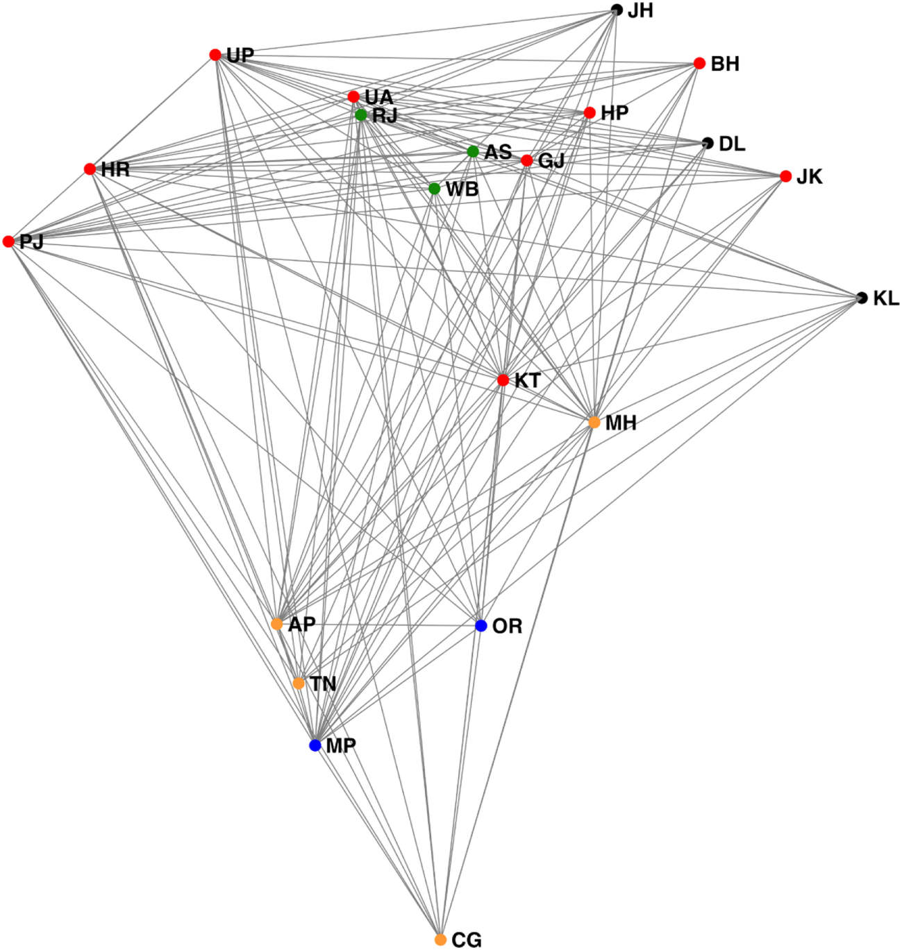
Figure 1

Spectral layout of Indian states according to total virtual water flow, with directed spectral graph partitioning used to separate states into foodsheds. One foodshed is indicated as green, the other as orange, and nodes not part of the large strongly connected component are drawn in black.
Applying a first spectral bisection, we obtain the partition into two regions that are depicted in “flow space” in Figure 1 and depicted geographically in Figure 2. We find that modularity Q improves from 0 for the whole graph to 0.1656 after the first bisection. If we hierarchically do further bisection on either of the two regions as depicted in Figures 3 and 4, the modularity Q decreases to 0.0979 and to 0.0143, respectively. Thus, the natural partition of the virtual water flow network into foodsheds is just two foodsheds for India.
Figure 2
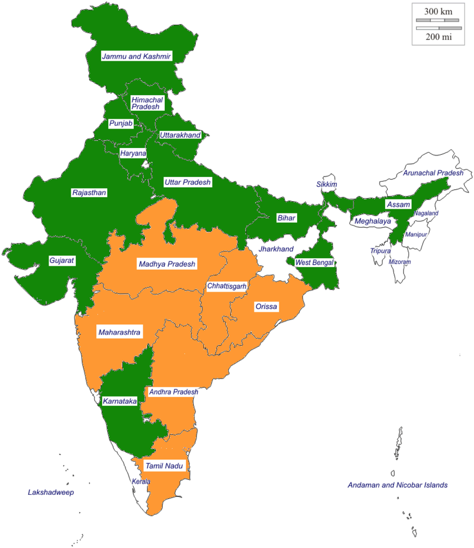
Geographic layout of two directed spectral foodsheds among the Indian states according to total virtual water flow. One foodshed is indicated as green, the other as orange, and states not part of the large strongly connected component or with missing data are drawn in white.
Figure 3
Spectral layout of Indian states according to total virtual water flow, with hierarchical directed spectral graph partitioning used to separate states into four regions. Regions are indicated as green, orange, red, and blue; nodes not part of the large strongly connected component are drawn in black.
Figure 4
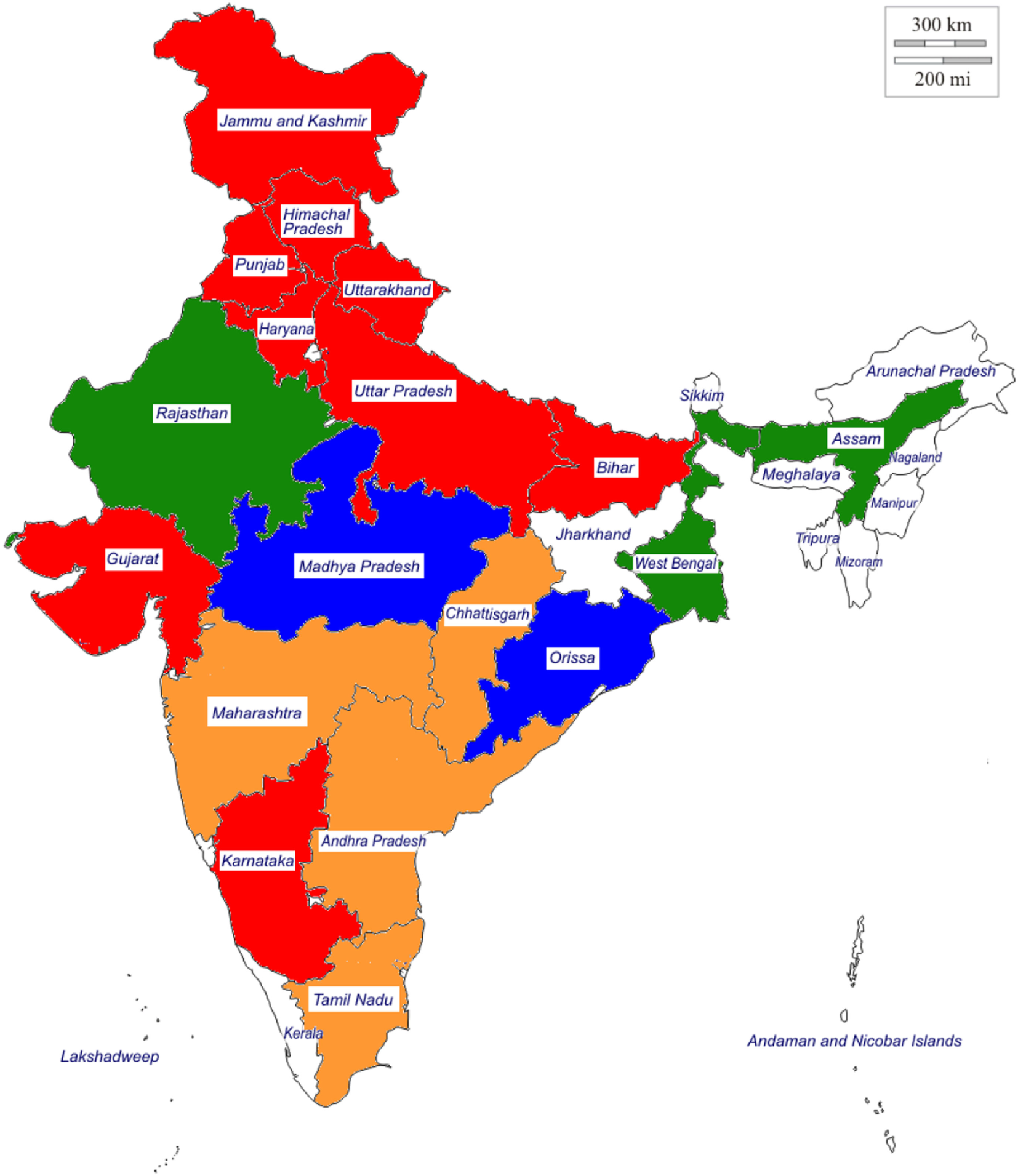
Geographic layout of directed spectral regions among the Indian states according to total virtual water flow. Regions are indicated as green, orange, red, and blue; states not part of the large strongly connected component or with missing data are drawn in white.
Although there are formal approaches for defining geographic continuity (Wu and Murray, 2008), we clearly observe that the two foodsheds of India are largely contiguous. Only Karnataka is geographically separated from other states in its foodshed.
Using the dataset and virtual water flow quantitation described above, we study virtual water flow among the United States of America in 2007. We find that spectral partitioning stops at two foodsheds like India, but that these foodsheds are not largely geographically contiguous, see Figure 5. Note that we believe there are errors in the 2007 Commodity Flow Survey Data for Indiana, which is why Indiana is not in the strongly connected component.
Figure 5
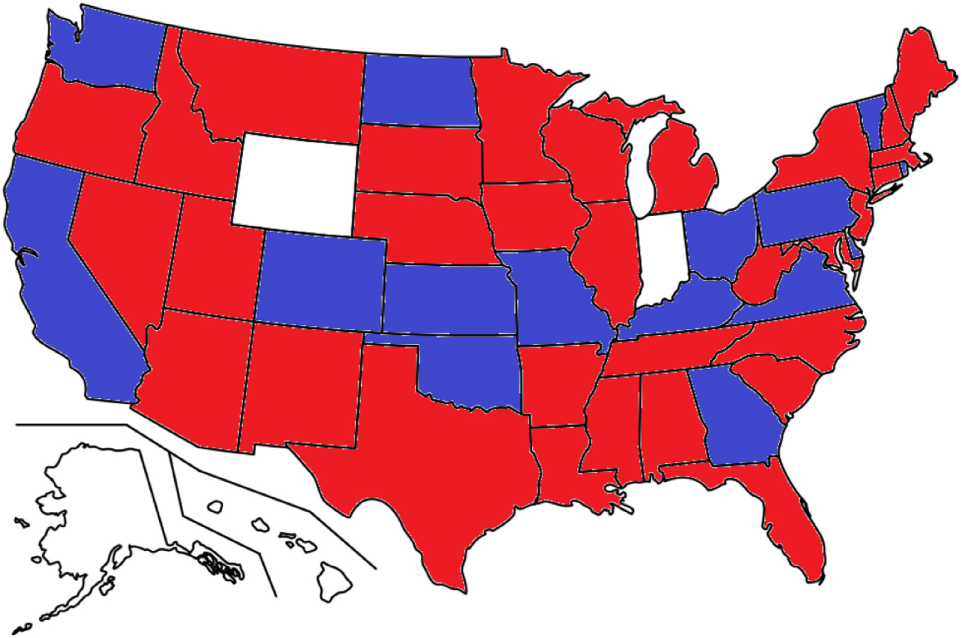
Geographic layout of directed spectral regions among the United States according to total virtual water flow. Regions are indicated as red and blue; states not part of the large strongly connected component or with missing data are drawn in white.
Using 2008 world data as described above, we repeat the same spectral bipartition analysis and end up with three foodsheds: two are fairly small and compact, whereas the other contains all other countries in the world. Note that many countries of the world are not part of the strongly connected component of global commerce. The first foodshed is in southern Africa and also includes Papua New Guinea. The second is largely around southwestern Asia and the Indian Ocean rim. See Table 2. Note that India (Goswami and Nishad, 2015) and the United States are major net exporters of water-intensive food crops in global trade. Thus, in a global characterization of foodsheds, these countries play central roles and are in fact in distinct global foodsheds.
Table 2
| 1 | Botswana, Malawi, Mozambique, Namibia, Papua New Guinea, Zimbabwe, South Africa, Swaziland, Zambia |
| 2 | Bhutan, Burundi, Sri Lanka, Egypt, India, Jordan, Kenya, Kuwait, Lebanon, Eritrea, Qatar, Rwanda, Saudi Arabia, Somalia, Sudan, Tanzania, Oman, United Arab Emirates, Uganda, Ethiopia, Yemen |
| 3 | Armenia, Afghanistan, Albania, Algeria, Angola, Argentina, Australia, Austria, Bangladesh, Bolivia, Brazil, Belize, Brunei, Bulgaria, Myanmar, Cameroon, Canada, Central African Republic, Chile, Colombia, Congo, Costa Rica, Cuba, Cyprus, Azerbaijan, Benin, Denmark, Dominican Republic, Belarus, Ecuador, El Salvador, Estonia, Finland, France, Georgia, Gabon, Gambia, Germany, Bosnia and Herzegovina, Ghana, Greece, Guatemala, Guinea, Guyana, Haiti, Honduras, Hungary, Croatia, Indonesia, Iraq, Ireland, Israel, Italy, Cote d’Ivoire, Jamaica, Japan, Kyrgyzstan, Cambodia, Republic of Korea, Latvia, Laos, Liberia, Lithuania, Madagascar, Malaysia, Mali, Mauritania, Mexico, Mongolia, Morocco, Moldova, Nepal, Netherlands, Macedonia, New Zealand, Nicaragua, Niger, Nigeria, Norway, Pakistan, Panama, Czech Republic, Paraguay, Peru, Philippines, Poland, Portugal, Romania, Russia, Senegal, Sierra Leone, Slovenia, Slovakia, Spain, Suriname, Tajikistan, Sweden, Switzerland, Syrian Arab Republic, Turkmenistan, Thailand, Togo, Trinidad and Tobago, Tunisia, Turkey, United Kingdom, Ukraine, United States of America, Burkina Faso, Uruguay, Uzbekistan, Venezuela, Vietnam, Belgium, Luxembourg, China |
Foodsheds from 2008 world trade data.
5 Conclusion
In this paper, we have put forth a formal data-driven definition of foodsheds from network science and computed foodsheds for India, the United States, and the world. We found that the Indian foodsheds are largely geographically contiguous, in the sense that states within foodsheds all border each other. Note that this notion of contiguity implicitly assumes the use of land transport, but ship-based transport may be more energy efficient (Van Passel, 2013). On the contrary, foodsheds in the United States are not nearly as contiguous, but some geographically compact foodsheds do emerge in the global flow data. However, in all three examples, the foodsheds are relatively large and indicate that both intranational and international food flows are highly connected between many states and nations.
Here, we defined foodsheds in terms of virtual water flow, but several alternative definitions could be considered, whether based on the tonnage of food itself, the total price of food, the virtual energy flow as embedded in food, or the negative externalities embedded in food. We expect that the results are fairly robust to the particular commensuration of flow used to define foodsheds. One can also further specialize data to consider, say, rice-sheds or potato-sheds. One may even be able to extend spectral graph techniques for directed networks to the setting of multilayer networks, to consider several notions of flow simultaneously.
It is our contention that the formal data-driven methodology we proposed for defining foodsheds can be used more broadly to study a variety of commodity flows and the impact these flows have on sustainability. Such information can be useful in developing environmentally oriented policies. Coming full circle, the effect of policy on foodshed boundaries can be visualized using the method we propose. That is, spectral graph partitioning of directed graphs may be a general analysis technique for sustainability science and public policy, cf., Hausmann et al. (2014).
Can we quantitatively determine which foodsheds are sustainable and which are not? We had noted that foodsheds are governed by the combined force of natural and social factors, and as we saw, we have contiguous (potentially sustainable) foodsheds if the natural geometry of the commodity flow network is essentially embeddable in the geographic adjacency network. That is, we may have sustainability, at least from the perspective of transport energy and externalities, if active human factors do not distort the natural way of things, as formalized in the sense of graph embedding.
Statements
Author contributions
Both authors contributed to all aspects of the paper.
Acknowledgments
We thank Prof. Megan Konar for providing the world virtual water flow data from Konar et al. (2011, 2012), for walking us through the U.S. commodity flow data, and for discussions.
Conflict of interest
The authors declare that the research was conducted in the absence of any commercial or financial relationships that could be construed as a potential conflict of interest.
Footnotes
1.^ The above connections are not meant to be exhaustive, but rather illustrate some of the ways in which these resources are fundamentally linked.
2.^ Not only can water be embedded in food but energy can also be embedded in water, as the ice trade of yore demonstrates (Cummings, 1949): there really is a nexus not just at the level of public policy, but in the commodities themselves.
3.^ Food transport over land may, however, be more energetically and environmentally costly than over water. Thus, we should take care in interpreting results.
4.^ The CFS is a collaborative effort between the Department of Transportation Statistics and the Census Bureau.
References
1
Chung F. (2005). Laplacians and the Cheeger inequality for directed graphs. Ann. Comb.9, 1–19.10.1007/s00026-005-0237-z
2
Cronon W. (1991). Nature’s Metropolis: Chicago and the Great West. New York: W. W. Norton & Company.
3
Cummings R. O. (1949). The American Ice Harvest: A Historical Study in Technology, 1800–1918. Berkeley: University of California Press.
4
Dang Q. Lin X. Konar M. (2015). Agricultural virtual water flows within the United States. Water Resour. Res.51, 973–986.10.1002/2014WR015919
5
Dingman S. L. (2002). Physical Hydrology, 2nd Edn. Upper Saddle River, NJ: Prentice Hall.
6
Gleich D. F. (2006). Hierarchical Directed Spectral Graph Partitioning. Information Networks, Final Project. Stanford, CA: Stanford University.
7
Goswami P. Nishad S. N. (2015). Virtual water trade and time scales for loss of water sustainability: a comparative regional analysis. Sci. Rep.5, 9306.10.1038/srep09306
8
Hall K. M. (1970). An r-dimensional quadratic placement algorithm. Manage. Sci.17, 219–229.10.1287/mnsc.17.3.219
9
Hausmann R. Hidalgo C. A. Bustos S. Coscia M. Simoes A. Yildirim M. A. (2014). The Atlas of Economic Complexity. Cambridge, MA: MIT Press.
10
Hedden W. P. (1929). How Great Cities are Fed. Boston: D.C. Heath and Company.
11
Hoekstra A. Y. Chapagain A. K. (2008). Globalization of Water: Sharing the Planet’s Freshwater Resources. Malden, MA: Wiley-Blackwell.
12
Horst M. Gaolach B. (2015). The potential of local food systems in North America: a review of foodshed analyses. Renew. Agric. Food Syst.30, 399–407.10.1017/S1742170514000271
13
Hughes T. P. (1985). Networks of Power: Electrification in Western Society, 1880–1930. Baltimore: Johns Hopkins University Press.
14
Jensen M. E. (1968). “Water consumption by agricultural plants,” in Water Deficits and Plant Growth, ed. KozlowskiT. T. (New York: Academic Press), 1–22.
15
Kampman D. A. (2007). The Water Footprint of India: A Study on Water Use in Relation to the Consumption of Agricultural Goods in the Indian States. M.Sc. Essay, University of Twente, Enschede.
16
Koehler A. (2008). Water use in LCA: managing the planet’s freshwater resources. Int. J. Life Cycle Assess.13, 451.10.1007/s11367-008-0028-6
17
Konar M. Dalin C. Hanasaki N. Rinaldo A. Rodriguez-Iturbe I. (2012). Temporal dynamics of blue and green virtual water trade networks. Water Resour. Res.48, W07509.10.1029/2012WR011959
18
Konar M. Dalin C. Suweis S. Hanasaki N. Rinaldo A. Rodriguez-Iturbe I. (2011). Water for food: the global virtual water trade network. Water Resour. Res.47, W05520.10.1029/2010WR010307
19
Koren Y. (2005). Drawing graphs by eigenvectors: theory and practice. Comput. Math. Appl.49, 1867–1888.10.1016/j.camwa.2004.08.015
20
Leicht E. A. Newman M. E. J. (2008). Community structure in directed networks. Phys. Rev. Lett.100, 118703.10.1103/PhysRevLett.100.118703
21
Lin X. Dang Q. Konar M. (2014). A network analysis of food flows within the United States of America. Environ. Sci. Technol.48, 5439–5447.10.1021/es500471d
22
Malliaros F. D. Vazirgiannis M. (2013). Clustering and community detection in directed networks: a survey. Phys. Rep.533, 95–142.10.1016/j.physrep.2013.08.002
23
Mekonnen M. M. Hoekstra A. Y. (2011). The green, blue and grey water footprint of crops and derived crop products. Hydrol. Earth Syst. Sci.15, 1577–1600.10.5194/hess-15-1577-2011
24
Mubako S. T. (2011). Frameworks for Estimating Virtual Water Flows among U.S. States. Ph.D. thesis, Southern Illinois University, Carbondale.
25
Peters C. J. Bills N. L. Wilkins J. L. Fick G. W. (2009). Foodshed analysis and its relevance to sustainability. Renew. Agric. Food Syst.24, 1–7.10.1017/S1742170508002433
26
Pretty J. N. Ball A. S. Lang T. Morison J. I. L. (2005). Farm costs and food miles: an assessment of the full cost of the UK weekly food basket. Food Policy30, 1–19.10.1016/j.foodpol.2005.02.001
27
Van Passel S. (2013). Food miles to assess sustainability: a revision. Sustain. Dev.21, 1–17.10.1002/sd.485
28
Varshney L. R. (2013). The wiring economy principle for designing inference networks. IEEE J. Sel. Areas Commun.31, 1095–1104.10.1109/JSAC.2013.130611
29
Volpe R. Roeger E. Leibtag E. (2013). How Transportation Costs Affect Fresh Fruit and Vegetable Prices. Economic Research Report 160. Washington, DC: United States Department of Agriculture.
30
Wu X. Murray A. T. (2008). A new approach to quantifying spatial contiguity using graph theory and spatial interaction. Int. J. Geogr. Inf. Sci.22, 387–407.10.1080/13658810701405615
Summary
Keywords
data, food, virtual water, water, spectral graph theory
Citation
Kshetry N and Varshney LR (2017) Foodsheds in Virtual Water Flow Networks: A Spectral Graph Theory Approach. Front. ICT 4:17. doi: 10.3389/fict.2017.00017
Received
04 February 2017
Accepted
09 June 2017
Published
26 June 2017
Volume
4 - 2017
Edited by
Tom Crick, Cardiff Metropolitan University, United Kingdom
Reviewed by
Gokarna Sharma, Kent State University, United States; Jonathan Gillard, Cardiff University, United Kingdom
Updates
Copyright
© 2017 Kshetry and Varshney.
This is an open-access article distributed under the terms of the Creative Commons Attribution License (CC BY). The use, distribution or reproduction in other forums is permitted, provided the original author(s) or licensor are credited and that the original publication in this journal is cited, in accordance with accepted academic practice. No use, distribution or reproduction is permitted which does not comply with these terms.
*Correspondence: Lav R. Varshney, varshney@illinois.edu
Specialty section: This article was submitted to Big Data, a section of the journal Frontiers in ICT
Disclaimer
All claims expressed in this article are solely those of the authors and do not necessarily represent those of their affiliated organizations, or those of the publisher, the editors and the reviewers. Any product that may be evaluated in this article or claim that may be made by its manufacturer is not guaranteed or endorsed by the publisher.