 Loyce Kayanula
 Kristan Alexander Schneider
- 1Department of Applied Computer and Biosciences, University of Applied Sciences Mittweida, Mittweida, Germany
- 2Center for Global Health, Department of Internal Medicine, School of Medicine, University of New Mexico, Albuquerque, NM, United States
- 3Translational Informatics Division, Department of Internal Medicine, School of Medicine, University of New Mexico, Albuquerque, NM, United States
- 4Clinical and Translational Science Center, Health Science Center, University of New Mexico, Albuquerque, NM, United States
Introduction: The presence of multiple genetically distinct variants (lineages) within an infection (multiplicity of infection, MOI) is common in infectious diseases such as malaria. MOI is considered an epidemiologically and clinically relevant quantity that scales with transmission intensity and potentially impacts the clinical pathogenesis of the disease. Several statistical methods to estimate MOI assume that the number of infectious events per person follows a Poisson distribution. However, this has been criticized since empirical evidence suggests that the number of mosquito bites per person is over-dispersed compared to the Poisson distribution.
Methods: We introduce a statistical model that does not assume that MOI follows a parametric distribution, i.e., the most flexible possible approach. The method is designed to estimate the distribution of MOI and allele frequency distributions from a single molecular marker. We derive the likelihood function and propose a maximum likelihood approach to estimate the desired parameters. The expectation maximization algorithm (EM algorithm) is used to numerically calculate the maximum likelihood estimate.
Results: By numerical simulations, we evaluate the performance of the proposed method in comparison to an established method that assumes a Poisson distribution for MOI. Our results suggest that the Poisson model performs sufficiently well if MOI is not highly over-dispersed. Hence, any model extension will not greatly improve the estimation of MOI. However, if MOI is highly over-dispersed, the method is less biased. We exemplify the method by analyzing three empirical evidence in P. falciparum data sets from drug resistance studies in Venezuela, Cameroon, and Kenya. Based on the allele frequency estimates, we estimate the heterozygosity and the average MOI for the respective microsatellite markers.
Discussion: In conclusion, the proposed non-parametric method to estimate the distribution of MOI is appropriate when the transmission intensities in the population are heterogeneous, yielding an over-dispersed distribution. If MOI is not highly over-dispersed, the Poisson model is sufficiently accurate and cannot be improved by other methods. The EM algorithm provides a numerically stable method to derive MOI estimates and is made available as an R script.
1 Introduction
Malaria and similar infectious diseases often exhibit a complex landscape of pathogen genetic diversity within individual infections. In malaria, the presence of multiple genetically distinct pathogen variants within a single infection is typically referred to as complexity of infection (COI) or multiplicity of infection (MOI) (Read and Taylor, 2001; Chang et al., 2017; Schneider, 2018). MOI is commonly reported in the context of malaria molecular surveillance, which has become increasingly popular in the last years as molecular assays become more affordable in endemic settings and due to WHO recommendations (World Health Organization, 2022; Sinha et al., 2023).
Epidemiologically, MOI is an important parameter as it scales with transmission intensities, however not necessarily in a linear way (Pacheco et al., 2020; Sinha et al., 2023). The effect of interactions of different pathogen variants within infections (intra-host dynamics) has been considered important in several theoretical models (e.g., Hastings and Watkins, 2005; Gurarie and McKenzie, 2006). However, so far, empirical evidence on the impact of MOI on the clinical pathogenesis of malaria remains inconclusive (Pacheco et al., 2016). Nevertheless, the distribution of MOI influences the evolutionary dynamics of malaria (Schneider, 2021; Schneider and Salas, 2022) and mediates evolutionary–genetic patterns and pathogen genetic diversity (e.g., patterns of genetic hitchhiking and linkage disequilibrium) as it affects the effective rate of recombination as illustrated in Figure 1 (Schneider and Kim, 2010; Alizon et al., 2013). Moreover, there is an important link between the frequency distribution of pathogen variants, their occurrence within infections (i.e., prevalence), and MOI. Specifically, given the frequency of a certain pathogen variant, its prevalence increases with MOI. This is particularly relevant in the context of anti-malarial drug resistance and seasonal malaria with varying transmission intensities (Geiger et al., 2014; Schneider, 2021; Schneider et al., 2022).
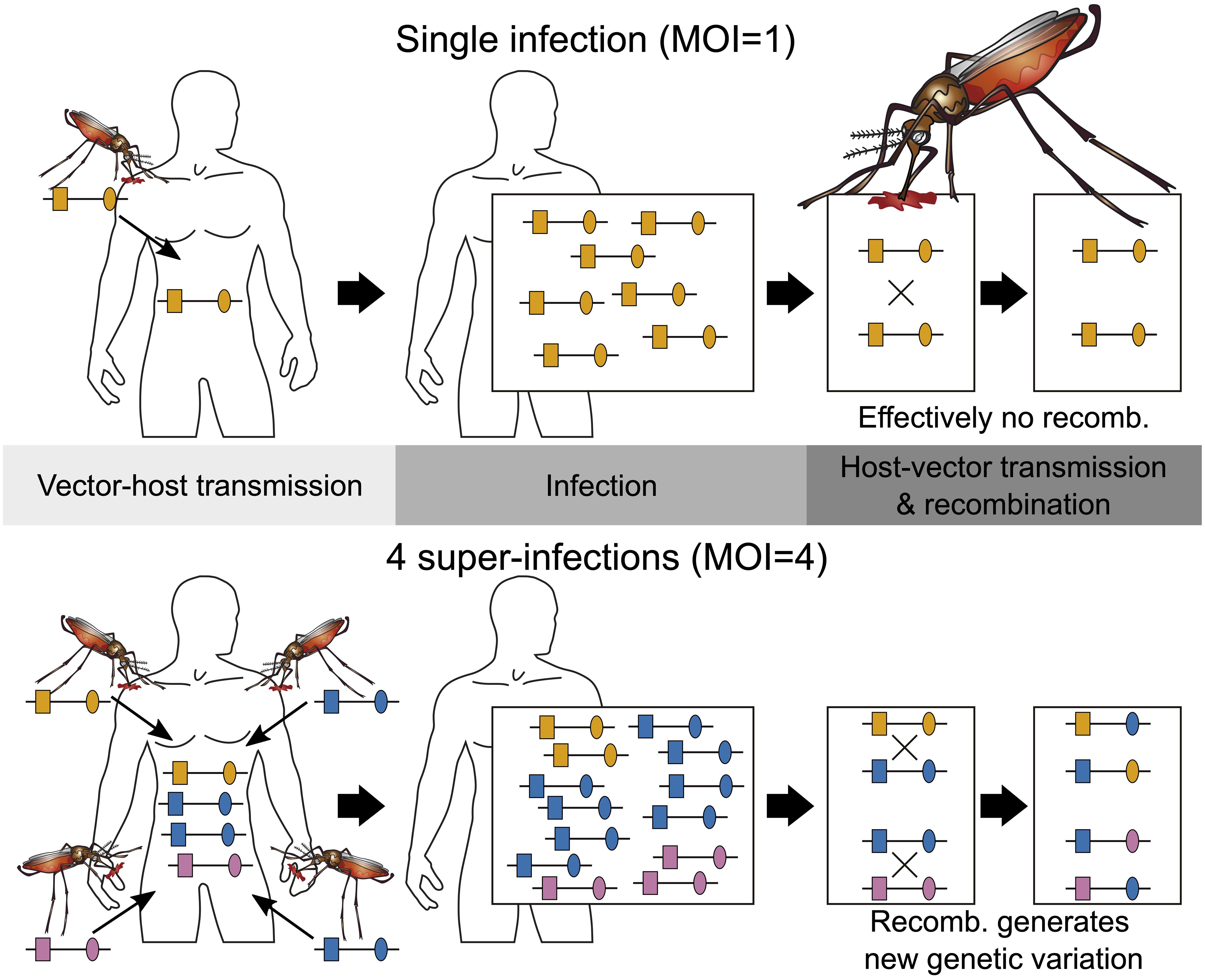
Figure 1 Illustration of MOI: Illustrated are two infections with MOI = 1 (single infection) shown on the top and MOI = 4 (multiple infection) shown on the bottom. Single infections lead effectively to no recombination. Note that the host on the bottom is infected twice with the same lineage. Because there are three different lineages in the infection, recombination can happen during host–vector transmission.
Importantly, MOI or COI is not unambiguously defined. Several formulations of MOI exist, with discrepancies between verbal and formal definitions (which typically underlay statistical models) as discussed in detail in Schneider et al. (2022). Here we follow the suggested definition in Schneider et al. (2022), which is used in most theoretical frameworks. Particularly, MOI is not defined as the number of distinct pathogen variants within an infection but as the number of “super-infections” during one disease episode. More precisely, MOI is the number of independent infectious events, assuming that exactly one pathogen variant (lineage) is transmitted per event (Hill and Babiker, 1995; Schneider and Escalante, 2014). This implies that MOI is an unobservable quantity because a host can be infected multiple times with the same pathogen variant (Figure 1), and these infectious events cannot be reconstructed from molecular assays (Figure 2). Notably, as pointed out in Schneider et al. (2022), if the distribution of MOI in the population is known or estimated, the distribution of different pathogen variants within infections can be derived (but not vice versa). The definition of MOI used here only approximately accounts for “co-infections”, i.e., the co-transmission of several pathogenic variants during an infective episode (Schneider, 2021). Focusing on super-infections (and only approximately covering co-infections) has the pragmatic advantage that no explicit model of vector–host transmission has to be specified (Schneider, 2021) considering that a co-infection is particularly relevant if one aims to determine the genetic relatedness of pathogen variants within an infection. To obtain enough resolution to study genetic relatedness, these approaches require high-quality genomic data. Although such approaches have become increasingly popular in the last years (cf. Nkhoma et al., 2012; Wong et al., 2018; Zhu et al., 2019; Nkhoma et al., 2020; Dia and Cheeseman, 2021; Neafsey et al., 2021), these approaches are inappropriate if only a handful of genetic markers are available.
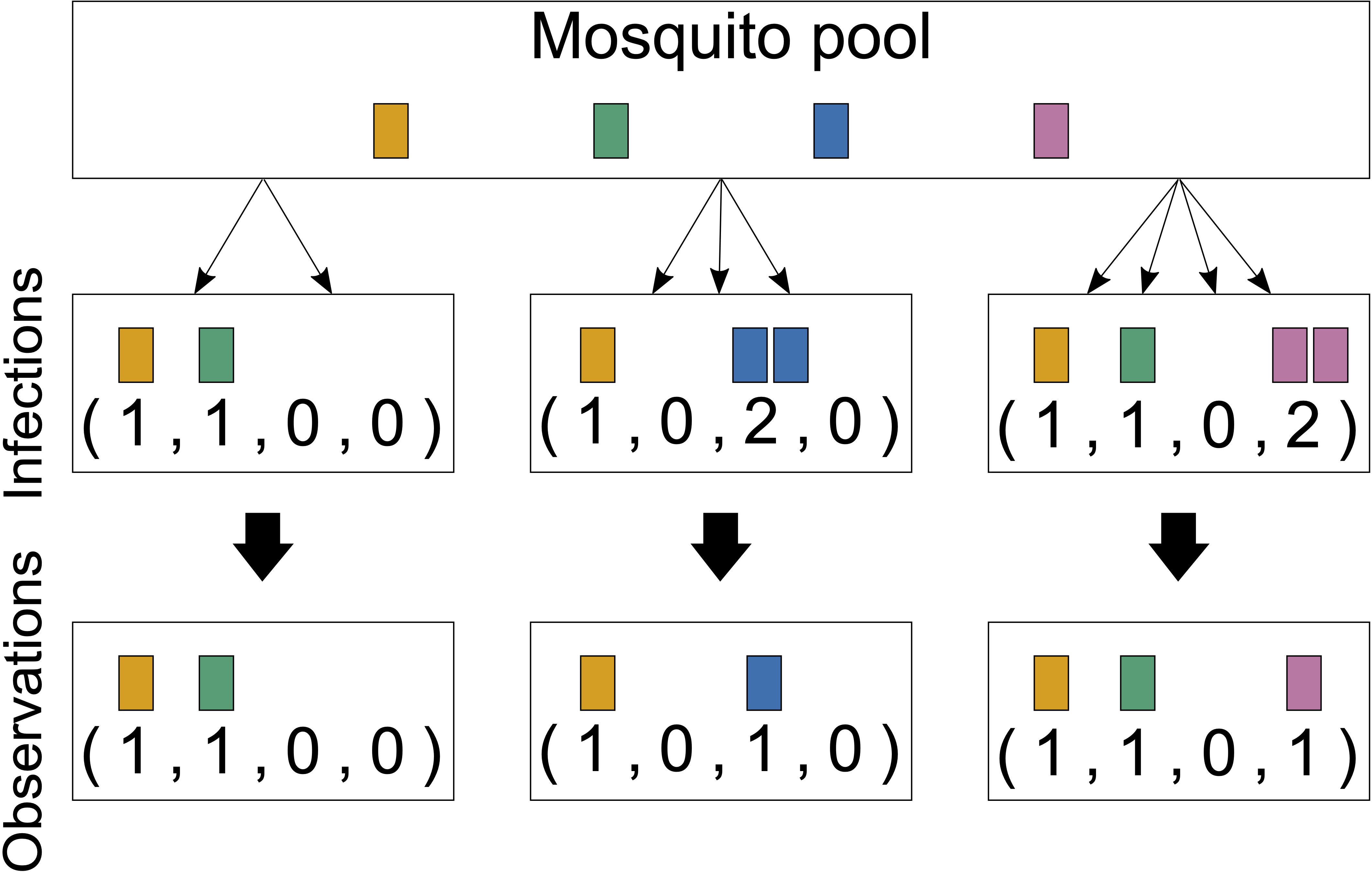
Figure 2 Infections and observations: Illustrated are three infections from four lineages circulating in the pathogen population. The first infection has MOI = 2 and contains two distinct pathogen variants. The second infection has MOI = 3, but only with two distinct pathogen variants, and the third has MOI = 4 and contains three distinct pathogen variants. Only the presence or absence of variants can be observed by molecular assays. The number of times that each lineage was transmitted cannot be reconstructed from a sample; generally, MOI is unobservable.
Heuristic methods to estimate the distribution of MOI are typically biased; methods based on a solid statistical framework are preferable (Schneider, 2021). Several such methods (which are essentially based on the same statistical framework) have been proposed to estimate the MOI and lineage frequencies for various assumptions concerning the genetic architecture of the underlying molecular data. All these methods make certain assumptions on the distribution of MOI in the population. The maximum likelihood-based method of Hill and Babiker (1995) assumes that MOI follows either a (conditional) Poisson or negative binomial distribution and is based on one or two genetic markers. In the case of MOI following a positive Poisson distribution, this method was refined by applying a bias correction in the case of a single molecular marker by Hashemi and Schneider (2021) and to an arbitrary number of biallelic molecular markers (Tsoungui Obama and Schneider, 2022). Moreover, the approach of Li et al. (2007) assumes that MOI follows a (conditional) Poisson distribution. The Bayesian method in the program COIL (Galinsky et al., 2015) and its generalization THE REAL McCOIL (Chang et al., 2017) does not explicitly specify a specific distribution for MOI per se, but the implementation imposes a uniform distribution, which constrains the resulting posterior distribution of MOI.
Under the assumption that infective mosquito bites are rare and independent in a population with homogeneous exposure, MOI follows a Poisson distribution. This renders this parametric choice an important null model. However, if mosquito biting rates are heterogeneous in the population, the distribution of MOI will more likely follow a mixture of Poisson or a negative binomial distribution (Schneider et al., 2022). In fact, empirical evidence indicates that mosquito biting patterns are heterogeneous, with certain individuals experiencing more bites than others. This is influenced by confounding factors such as environmental conditions or individual attractiveness to mosquitoes (Noor et al., 2014; Guelbeogo et al., 2018). Consequently, the number of mosquito bites per person tends to be over-dispersed compared to the Poisson distribution (Irvine et al., 2018). (Note, however, that an over-dispersed mosquito biting rate does not imply that the MOI distribution is over-dispersed, as it is concerned only with the number of infective bites.) In any case, significant deviations from the Poisson assumptions suggest that the negative binomial distribution might be more suitable (Lloyd-Smith, 2007). However, maximum likelihood estimation of the negative binomial distribution in general is problematic. As mentioned in Adamidis (1999), if the empirical variance is not larger than the mean of count data, the maximum likelihood estimates of the parameters of the negative binomial distribution are degenerate. A way to overcome the problem that estimation of both parameters can compromise the stability and interpretability of a negative binomial model (Bandara et al., 2019) is to estimate only one parameter, while fixing the other, as suggested in Piegorsch (1990), Saha and Paul (2005), and Lloyd-Smith (2007). In practice, this means that there needs to be prior information on one parameter. However, this is typically not feasible in the context of MOI because it would require additional information such as mosquito biting rates or host exposure to mosquitoes. Such information is typically beyond the scope of malaria molecular surveillance.
If there is a prior belief that MOI does not follow a Poisson distribution, rather than assuming that MOI falls into a different class of parametric distributions, such as the negative binomial distribution, no particular class of distributions has to be imposed. Such a non-parametric approach offers a valid alternative if the MOI is completely unknown because of its flexibility. In fact, a non-parametric approach is the most flexible approach in this context.
Here we introduce a non-parametric statistical model to estimate the distribution of MOI and pathogen lineage (allele) frequencies from a single molecular marker by maximum likelihood. Non-parametric refers to the fact that the MOI distribution is not assumed to fall into a class of parametric distributions. The statistical model is first introduced in “Materials and methods”. Because the resulting likelihood function is too complex to have a closed-form solution, we derive the expectation maximization algorithm (EM algorithm) to derive the maximum likelihood estimate (MLE) numerically (Couvreur, 1997; Ng et al., 2012). The EM algorithm provides a numerically stable iteration to derive the MLE. By numerical simulations, we further investigate the performance of the non-parametric estimator in terms of bias and variance and contrast it to MOI estimates based on the assumption of an underlying Poisson distribution. The method proposed here is further applied to three data sets from Cameroon, Kenya, and Venezuela as an illustration. The method is implemented as an R script available in the Supplementary Material and at https://github.com/Maths-against-Malaria/Non-parametric-MOI-estimation.
2 Materials and methods
In the following mathematical notation, we use oblique letters, e.g., m, p, x, to indicate vectors, and italic fonts, e.g., m, p, x, to refer to integers or scalars.
We consider a pathogen population with lineages A1, …, An, detected at a single marker locus. Each lineage (or allele) Ai has relative frequency pi in the pathogen population, jointly denoted by the vector p = (p1, …, pn). We assume that at each infective event, the mosquito vector transmits exactly one lineage to the host. This corresponds to randomly sampling one lineage from the pathogen population. Hence, co-infections (cf. Figure 1 in Schneider et al., 2022), i.e., the co-transmission of several distinct lineages during one infective event, are ignored. However, hosts can be infected multiple times by different mosquitoes (super-infections) during one disease episode. It is assumed that super-infections occur during relatively short time periods, e.g., a few days, so that all infecting variants reach detectable concentrations. Infective events, in which the variants do not reach detectable frequencies, do not count as super-infection as these (i) are irrelevant for the clinical pathogenesis of the disease and (ii) are undetectable by molecular assays. Following Schneider et al. (2022), we refer to the number of infective events during one disease episode as multiplicity of infection (MOI). Importantly, the hosts might be infected multiple times with the same lineage. Formally, if mi represents the number of times an individual was infected with lineage Ai, then mi = 0 if the host was not infected with lineage Ai. Summing over all mi yields MOI m, i.e., MOI m is defined by:
where m = (m1, …, mn). The m lineages infecting a host are randomly sampled (with replacement) from the pathogen population. Therefore, within an infection, the configuration of pathogen lineages m follows a multinomial distribution with parameters m = |m| and p, i.e., m ∼ Multi (m,p). Hence, given that a host has MOI m, the probability of configuration m, i.e., of being infected mi times with lineage Ai (i = 1,…, n), is:
where in Equation 1 is the multinomial coefficient and .
The configuration of infecting pathogen lineages (m) and even MOI (m = |m|) is unobservable. Specifically, from a blood sample of an infected person, the observation is limited to the absence/presence of the infecting lineages (Figure 2). Formally, we represent an observation as the vector x = (xi), i = 1,…, n, such that the entries xi are 0 or 1 (formally, xi∈ {0,1}), where 0 denotes the absence and 1 denotes the presence of the lineages in the infection (Figure 2). Thus, xi is the sign of mi, i.e., xi = 0 if mi = 0 and xi = 1 if mi≥ 1 (formally, xi := sign mi, or in compact notation x = sign m).
Because we consider only disease-positive samples, the observations x correspond to vectors of length n with entries 0 and 1 excluding the vector that contains only zeros, 0, which corresponds to a disease-negative sample. In mathematical notation, x are elements of the set 𝒪 := {0,1}n \ {0}.
The underlying assumption is that molecular/genetic methods are not quantifying the concentration of lineages but rather detect their presence. Here it is ignored that lineages remain undetected. While this can be included in a statistical model (see, e.g., Hashemi and Schneider, 2024), here it is ignored. For more discussion on undetected or erroneously detected variants, see Schneider et al. (2022).
To express the probability of x, further notation is needed. We call an observation y ∈ 𝒪 a sub-observation of x (denoted y ≼ x); all lineages observed in y are also observed in x, i.e., if yi ≤ xi for i = 1,…, n. The set of all sub-observations of x is denoted by:
We define κm := P[MOI = m] as the probability that a host is infected exactly m times (MOI = m) and collectively denote the MOI distribution by κ : = (κ1,κ2,…). Furthermore, the probability generating function (PGF) of the MOI distribution evaluated at a point z is denoted by G(z) (see “Probability distribution of observations” in the Appendix); the probability of observation x is derived to be as:
where we jointly denote the model parameters by and for to emphasize the dependency on the model parameters whenever necessary. Clearly, the probability in (Equation 2) depends on the model parameters p and κ (through the PGF).
Note that while piis the frequency of lineage Ai, as shown in Schneider et al. (2022), its prevalence, i.e., the probability that this lineage occurs in an infection, is given by
i.e., the PGF of the MOI distribution links frequency and prevalence.
The model parameters θ, i.e., the distribution of MOI and the lineage frequency distribution, can be estimated from the probabilistic model (Equation 2). We proceed with maximum likelihood (ML) estimation.
2.1 Likelihood function
Considering N independent observations x(1), …, x(N) from disease-positive hosts, collectively denoted as , the likelihood function (θ; ) is given by
In practice, the same allele configuration x can be observed in several hosts. Let nx be the number of times observation x occurs in the data. (Clearly, the total sample size N must be the sum over all , i.e., , where the sum runs over all possible observations.) With this notation, the likelihood function can be rewritten as
and the log-likelihood function becomes
The maximum likelihood estimate (MLE) of the true unknown parameter is the parameter vector that maximizes the likelihood or, equivalently, the log-likelihood function, i.e.,
Maximizing the log-likelihood function is infeasible without further restrictions because the model parameters θ are infinite-dimensional. The reason is that the distribution of MOI (κm) is infinite-dimensional. However, there are several meaningful strategies to restrict oneself to a finite-dimensional parameter space. A standard strategy is to assume that the MOI distribution falls into a parametric family and is hence characterized by finitely many model parameters—for instance, the simplest case is to assume that MOI follows a positive Poisson distribution and is hence characterized by a single parameter (cf. Hill and Babiker, 1995; Schneider and Escalante, 2014; Schneider, 2018; Hashemi and Schneider, 2021; Schneider, 2021; Schneider et al., 2022; Tsoungui Obama and Schneider, 2022). This, however, requires the additional assumption that infectious bites are rare and independent. A similar assumption is that MOI follows a positive negative binomial distribution and is hence characterized by two parameters (cf. Hill and Babiker, 1995; Schneider et al., 2022). The negative binomial distribution allows modeling over-dispersion in the number of infectious bites. However, since the observations will tend to look under-dispersed (because only absence/presence rather than MOI is observed), one needs to estimate the amount of over-dispersion from an additional data source. In principle, any other parametric distribution can be used.
In case there is no empirical argument that justifies the use of a specific parametric distribution, the MOI distribution can be just truncated by assuming a maximum MOI value M, i.e., κm = 0 for m > M. This is a reasonable assumption since κm will be negligible for large m anyway. We denote the MOI distribution by κ = (κ1, …, κM). In the following, we will pursue this non-parametric approach by restricting the admissible parameter space to the set of all possible MOI distributions with MOI values 1,2, … , M and all possible lineage frequency distributions, i.e.,
where SM and Sn denote the (M−1)− and (n−1)−dimensional simplices, respectively.
If there was no restriction on the maximum MOI value, the probabilistic model would be correct. The restriction renders the model to be only approximately correct—for instance, if the true MOI distribution follows a Poisson or negative binomial distribution, MOI can be any integer. Such a distribution can only be approximated by the probabilistic model above restricted to the parameter space Θ. However, by choosing the maximum MOI value M that is sufficiently large, any distribution can be approximated to any level of accuracy (cf. also Figure 3).
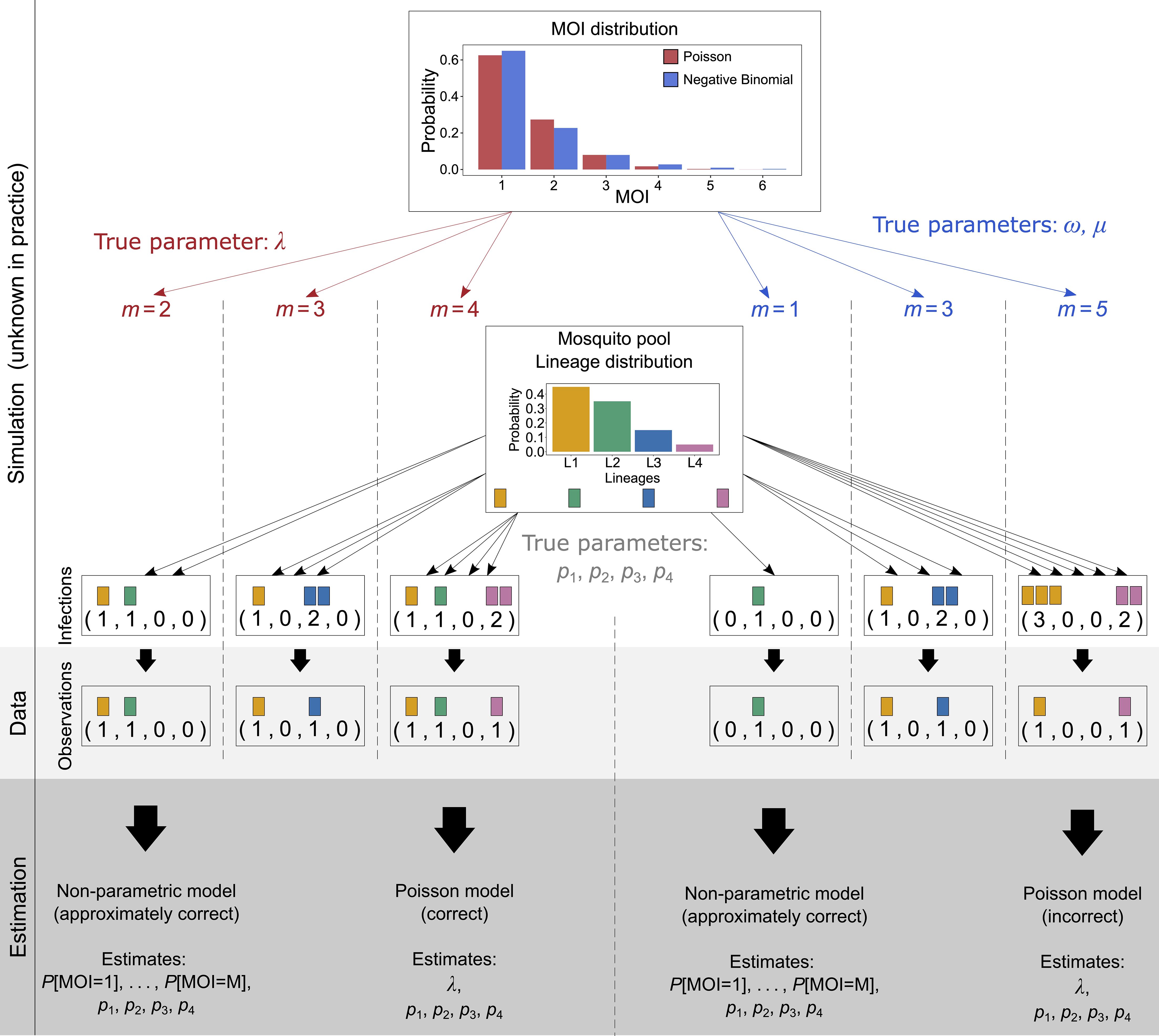
Figure 3 Illustration of simulated data: Illustrated is the simulation scheme for the numerical investigations. A sample of size N (N = 3 in the illustration) is created as follows: For a given MOI distribution, e.g., Poisson distribution (illustrated in red) or the negative binomial distribution (illustrated in blue), characterized by parameters, first N MOI values are randomly drawn (left-hand side for Poisson distribution and right-hand side for negative binomial distribution). For each of the MOI values, N infections are drawn. For MOI = m, exactly m lineages are drawn randomly from the lineage distribution, with replacement (multinomial distribution). The data of sample size N is then obtained by retaining only the information of absence and presence of lineages in the infection. From the resulting data, the model parameters are estimated. First, they are estimated by the non-parametric method, which is approximately correct, as it imposes a maximum MOI value M, which neither the Poisson nor the negative binomial distribution does. Therefore, these true underlying distributions are only approximated by the model. Second, the model parameters are estimated by the Poisson model, which estimates the lineage frequency distribution and the MOI parameter λ. This is the correct model if the true underlying distribution is actually a Poisson distribution (left-hand side), but it is incorrect if it is not (right-hand side). In the illustration, the negative binomial distribution is “approximated” by a Poisson distribution. The true (in practice unknown) parameter of the Poisson distribution was chosen to be λ = 0.5, and the parameters of the negative binomial distribution (µ = 0.67, ω = 2.08) were chosen; thus, the distribution is over-dispersed by 50%.
Unfortunately, the complexity of the log-likelihood function does not allow for an explicit solution of the MLE. The reason is that the derivatives of the log-likelihood function are polynomials in the lineage frequencies of degree up to M. Hence, the MLE must be derived numerically. We will further make use of the EM algorithm for this purpose.
The EM algorithm is derived in “Derivation of the Q-function” in the Appendix. In the present case, the algorithm estimates each probability κ1 = P[MOI = 1], κ2 = P[MOI = 2],…, κM = P[MOI = M] separately as well as the lineage frequencies p1,…, pn. The method is only approximately correct as we impose that M is the maximum possible MOI, i.e., κm = 0 for m > M.
2.2 Numerical investigations
Since there is no closed form for the MLE, we investigate the performance of the ML estimator by numerical simulations for a representative set of parameters. We further compare the performance of the ML estimator with that of Schneider and Escalante (2014), which assumes that the MOI follows a conditional Poisson distribution. Figure 3 illustrates how a data set is simulated, assuming that the true (in practice unknown) MOI distribution is either conditionally Poisson or negative binomially distributed.
For each choice of model parameters θ = (κ, p), we constructed K = 25, 000 data sets of sample size N = 50, 100, 200, and 300 according to the probabilistic model (Equation 2) (see Figure 3 for the construction of a data set of sample size N = 3, assuming that the underlying MOI distribution is either conditionally Poisson or negative binomially distributed). More precisely, for each of the N samples, first, the MOI value m was chosen randomly according to the distribution κ. For each MOI value m the MOI vector m was chosen randomly from a multinomial distribution with parameters m and p, and the corresponding observation was derived as x = sign m. This procedure was repeated K times. For a given set of parameters (N, κ, p), this resulted in K data sets (1), …, (K). For data set (k), we calculated the MLE from the non-parametric model according to Result 1, assuming a maximum MOI of M = 6 and the MLE according to the parametric model (Poisson model) of Schneider and Escalante (2014) using the implementation of Schneider (2018).
Let θ denote a component of the parameter vector θ. The relative bias of θ, defined by , was approximated by
where
i.e., the expectation which cannot be calculated because the MLE that has no closed form was approximated by the empirical mean over the K-simulated data sets.
Similarly, the variability of the estimator relative to the true parameters was assessed by the coefficient of variation (CV), i.e., as
The bias and variance for the parametric estimator were calculated in the same way with the necessary modifications.
The bias and variance of rare lineages might be substantial. However, the estimates of rare lineages that will be unlikely observed in practice have limited relevance. Therefore, we focus on reporting the bias and variance of the predominant lineage, i.e., of the largest lineage frequency, which is in practice an important quantity. Similarly, concerning the distribution of MOI κ, reporting bias and variance of small κm are not meaningful. However, also reporting on the MOI value with the highest frequency is not meaningful. Summary statistics such as the average MOI are of practical interest. The average MOI is not a model parameter but can be readily estimated by the plug-in estimator.
In the case of the parametric model, conditional Poisson model, the average MOI is estimated as . Here we report on the bias and variance of the average MOI estimated by the respective plug-in estimators.
2.3 Parameter choice
Besides the choices of K = 25, 000, sample sizes N = 50, 100, 200, and 300, as well as maximum MOI M = 6, we chose the model parameters p and κ as follows.
Concerning the lineage frequencies for n = 4 and n = 5 lineages, we chose the balanced and unbalanced frequency distributions (reported in Tables 1, 2). By balanced frequency distributions, we refer to instances in which each lineage has approximately the same frequency, whereas we refer to unbalanced distributions if there are one or more dominating lineages and one or more rare lineages.
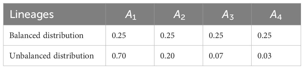
Table 1 Choice of n = 4 lineages and their corresponding balanced and unbalanced frequency distributions.

Table 2 Choice of n = 5 lineages and their corresponding balanced and unbalanced frequency distributions.
Concerning the distribution of MOI (κ), we assumed either a conditional Poisson distribution with parameter λ ranging from 0.1 to 2.9 in steps of 0.1 or a conditional negative binomial distribution with different degrees of over-dispersion. The parameters of the conditional negative binomial distribution were chosen such that the mean MOI matched those of the conditional Poisson distributions. For the Poisson distribution, the mean equals the variance (this is no longer true for the conditional Poisson distribution). For the negative binomial distribution with a scale parameter (ω) and shape parameter (µ), the variance is larger than the mean, i.e., it is over-dispersed. The amount of over-dispersion is
Regarding the parameter choices, we first chose as 1.05, 1.50, and 2, corresponding to 5%, 50%, and 100% over-dispersion. Then, we numerically matched the scale parameters such that the mean MOI of the corresponding conditional negative binomial distribution equals that of the conditional Poisson distribution. As an example, the conditional Poisson distribution in Figure 3 is λ = 0.9, and the corresponding negative binomial distribution is over-dispersed by 50%. Notably, it is impossible to find matching distributions if the mean MOI is too small. In other words, over-dispersion requires a sufficiently large mean MOI.
2.4 Model implementation
The statistical model is implemented in R (R Core Team, 2023) and available in the Supplementary Materials and on GitHub https://github.com/Maths-against-Malaria/Non-parametric-MOI-estimation, alongside a user-friendly documentation.
3 Results
First, it is shown how the maximum likelihood estimate (MLE) is derived. This is followed by results on the estimator’s performance in terms of bias and variance.
3.1 Deriving the MLE
The specific form of the likelihood function does not allow obtaining an explicit solution for the MLE. Specifically, assuming a maximum MOI of M, the derivatives of the likelihood function are polynomials in the model parameters of degree M − 1, for which no general solution of the roots exists. However, the MLE can be easily calculated numerically from the EM algorithm, which is derived in the Supplementary Materials [expectation maximization (EM) algorithm]. The EM algorithm provides a numerically stable and efficient iteration to calculate the MLE.
RESULT 1. Assume molecular information from N samples x(1), …, x(N). Furthermore, assume a maximum MOI value M. The MLE of the lineage frequency distribution p = (p1,…,pn) and the distribution of MOI κ = (κ1,…, κM), is calculated by the EM algorithm by performing the following steps:
1. Choose arbitrary initial conditions p(0) and κ(0);
2. In step t + 1, update the parameter choice p(t) and κ(t) by
and
where
and
with P[x|θ(t)] given by Equation 2 and G′ being the derivative of the PGF given by (A5).
3. Repeat step 2 until numerical convergence, e.g., ∥θ(t+1) − θ(t)∥< ϵ for some specified error threshold ε.
The EM algorithm converges fast in practice and is implemented as an R script.
3.2 Performance of the estimator
Only results for n = 4 lineages are presented here. The results for n = 5 lineages are similar and presented in the Supplementary Material (Appendix, Additional results; Supplementary Figures S2–S6).
3.2.1 Bias of lineage frequencies
The MLE of the lineage frequencies has very little bias (Equation 3) (Figures 4A, B, 5A–C, and 6A–C). Shown is only the bias of the dominant lineage (lineage 1). Bias is typically small for small average MOI, while the dominant lineage frequency tends to be overestimated if the true average MOI is large. However, bias vanishes with increasing sample size N. Bias tends to be larger for unbalanced lineage frequency distributions (cf. Figures 4A, B, 5A–C, and 6A–C). This is not surprising since for balanced frequency distributions all lineages are equivalent and should be present in equal amounts throughout the data. Importantly, the results are relatively robust with respect to the underlying true MOI distribution. While the bias is lowest from data generated from a conditional Poisson distribution (Figure 4), the bias remains similar if the data is generated from a conditional negative binomial distribution (Figures 5 and 6). However, the bias increases with increasing over-dispersion for unbalanced frequency distributions.
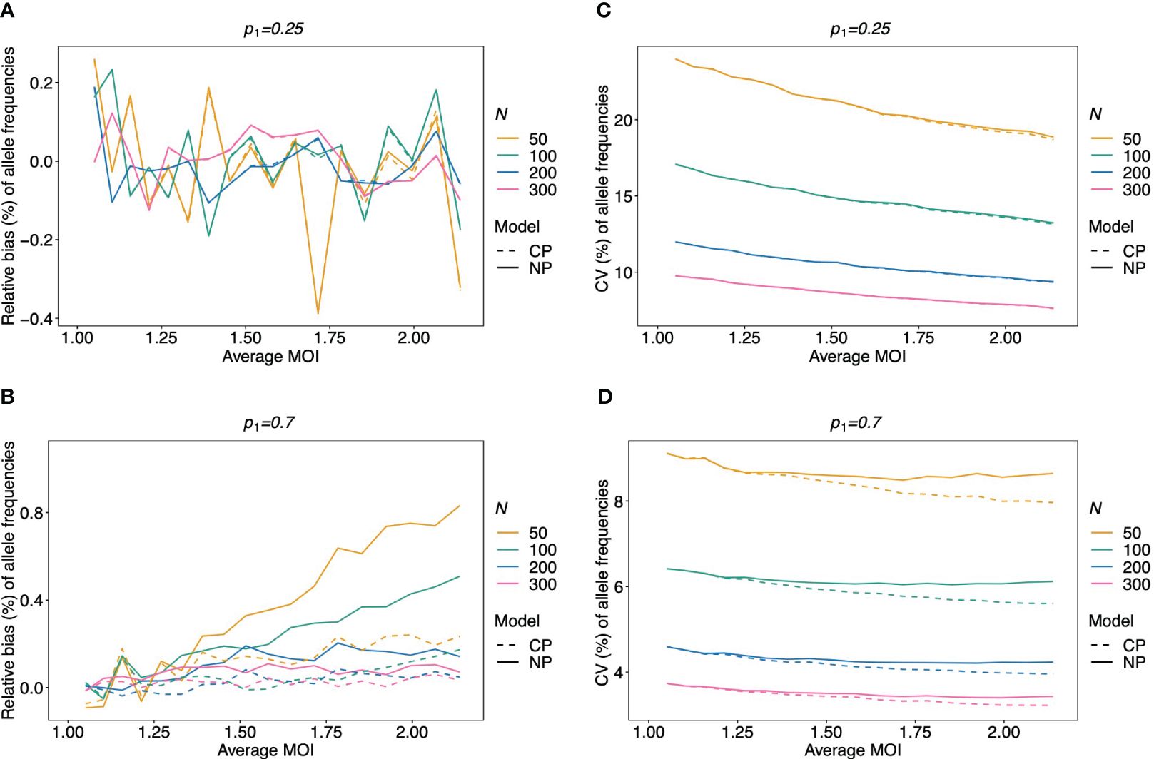
Figure 4 Relative bias and variation of MLE for pathogen lineage frequencies if MOI follows a Poisson distribution: Assumed are four lineages following the distributions in Table 1. (A, C) Balanced frequency distribution. (B, D) Unbalanced lineage frequency distribution. The dominant lineage frequency is shown at the top of the plot panels. The true MOI distribution in all panels follows a Poisson distribution with varying average MOI (x-axis). The panels show the relative bias (A, B) and CV (C, D) of the ML estimators of the dominant lineage frequency, based either on the non-parametric model (NP; solid lines) or the conditional Poisson model (CP; dashed lines) as functions of the true average MOI (cf. Figure 3) (note that the non-parametric model is only approximately correct in this case because a maximum MOI of M = 6 is assumed, while the Poisson model is correct). Colors correspond to different sample sizes.

Figure 5 Relative bias and variation of MLE for balanced pathogen lineage frequencies if MOI follows a negative binomial distribution: similar as in Figure 4. However, a balanced lineage frequency distribution is assumed here in each panel, and the true MOI distribution is a conditional negative binomial distribution with 5% (A, D), 50% (B, E), and 100% (C, F) over-dispersion. The gray-shaded areas indicate the parameter range which is impossible for a negative binomial distribution with the respective amount of over-dispersion. Note here that the non-parametric model (NP; solid lines) is still approximately correct, while the Poisson model (CP; dashed lines) is incorrect.
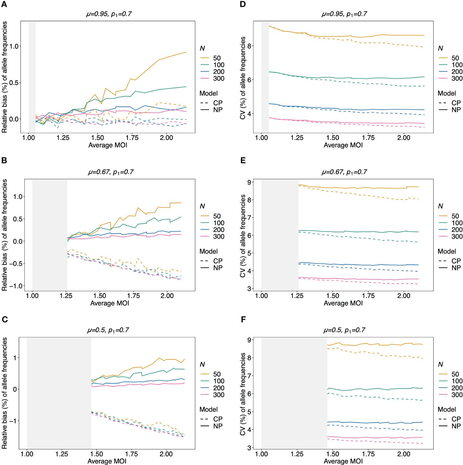
Figure 6 Relative bias and variation of MLE for unbalanced pathogen lineage frequencies if MOI follows a negative binomial distribution (A–F): see Figure 5, but for an unbalanced pathogen lineage distribution.
3.2.2 Variation of lineage frequencies
Not surprisingly, the variance of the MLE for the dominating lineage frequency—measured by the coefficient of variation (CV) (Equation 4)—decreases substantially with increasing sample size (Figures 4C, D, 5D, F, and 6D–F). For higher MOI, the CV tends to decrease slightly, which is not surprising since the data contains more information on the lineages. The CV tends to be smaller for unbalanced frequency distributions (cf. Figures 4C, D, 5D–F, and 6D–F) because the dominating lineage is present in more samples, increasing the information about its true frequency. The results seem to be robust with respect to the underlying true model, i.e., conditional Poisson and negative binomial model (Figures 5 and 6).
3.2.3 Frequency estimates by the non-parametric vs. conditional Poisson model
Given that MOI in infections follows a conditional Poisson distribution, the non-parametric model introduced here performs almost as good as the conditional Poisson model (Schneider and Escalante, 2014) (the correct model in this case). If the lineage frequency distributions are balanced, the two estimators perform equally well (Figures 4A, C). For unbalanced distributions, the correct model has only a slightly lower coefficient of variation and only for high average MOI. However, for a small sample size and high average MOI, the bias of the non-parametric model is higher (but still small) (Figures 4B, D).
Not surprisingly, if the true MOI distribution is over-dispersed compared to the Poisson distribution, the non-parametric model performs similarly to the conditional Poisson model if the lineage frequency distribution is balanced (Figure 5). However, the model outperforms the conditional Poisson model if the lineage frequency distributions are unbalanced. While the variances of the two estimators are comparable, the non-parametric estimates are less biased. This is intuitive because it is not constrained to an incorrect model. In fact, the Poisson model underestimates the dominant allele frequency (Figure 6; Supplementary Figure S7 for a comparison of the absolute bias). Importantly, while the relative bias decreases for the non-parametric model with increasing sample size, the opposite is observed for the conditional Poisson model (Figures 6B, C)
3.2.4 Bias of the estimates of average MOI
The bias of the average MOI (ψ) estimated by the non-parametric model is generally small (Figures 7A, B, 8A–C, and 9A–C) if the true average MOI is low to intermediate. There is a tendency for the average MOI to be overestimated for most of the parameters explored, with the bias decreasing with increasing sample size. Only for large average MOI does the true parameter tend to be underestimated. This underestimation is more pronounced for more over-dispersed MOI distributions (cf. Figures 7A, B, 8A, and 9A with Figures 8B, C and 9B, C). More precisely, the average MOI parameter is not underestimated if the MOI follows a conditional Poisson distribution for (almost) the whole range of parameters simulated, and the more over-dispersed the MOI distribution, the lower the threshold for which the average MOI is underestimated.
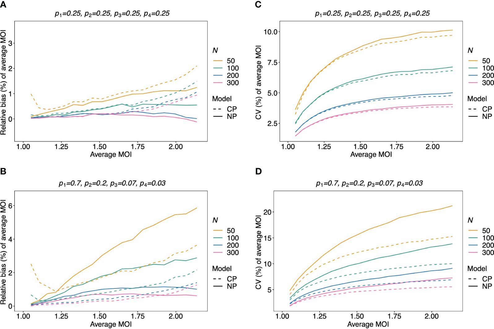
Figure 7 Relative bias and variation of the average MOI, if MOI follows a Poisson distribution: Assumed are four lineages with the distributions shown at the top of each panel [(A, C)—balanced; (B, D)—unbalanced distributions]. The true MOI distribution in all panels follows a Poisson distribution with varying average MOI (x-axis). The panels show the relative bias (A, B) and CV (C, D) of the ML estimators of the average MOI based either on the non-parametric model (NP; solid lines) or the conditional Poisson model (CP; dashed lines) as functions of the true average MOI (cf. Figure 3) (note that the non-parametric model is only approximately correct in this case because a maximum MOI of M = 6 is assumed, while the Poisson model is correct). Colors correspond to different sample sizes.
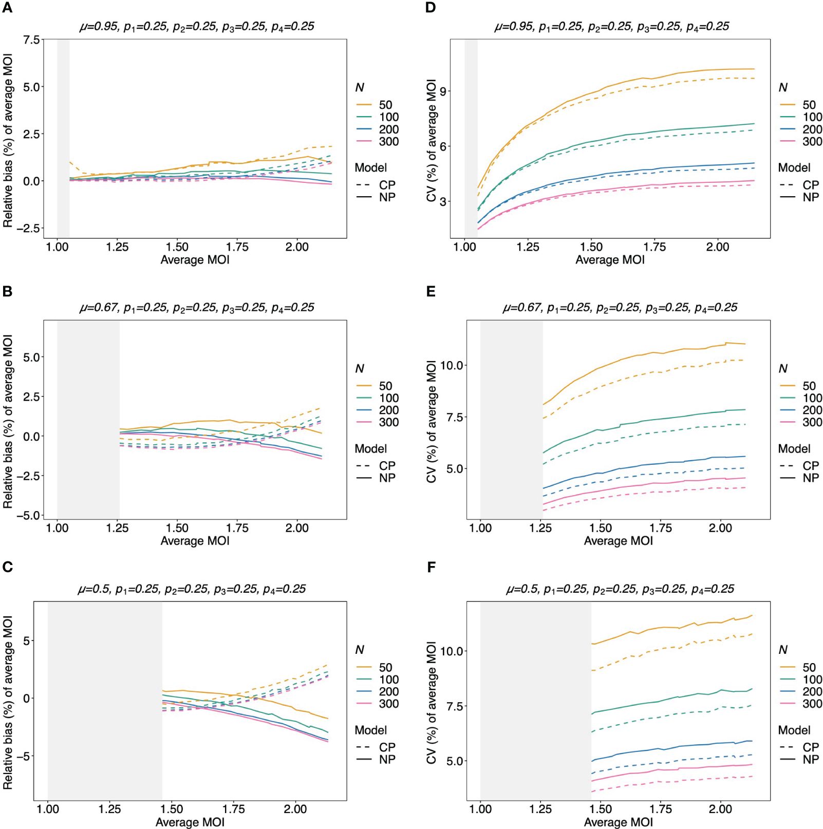
Figure 8 Relative bias and variation of the average MOI for balanced lineage frequencies if MOI follows a negative binomial distribution: similar as in Figure 7, but the true MOI distribution follows a negative binomial distribution with 5% (A, D), 50% (B, E), and 100% (C, F) over-dispersion and average MOI given on the x-axes. The corresponding model parameter µ is given at the top of each panel. All panels assume the same true balanced lineage frequency distribution (top of each panel). Note that the non-parametric model is approximately correct, while the Poisson model is incorrect.
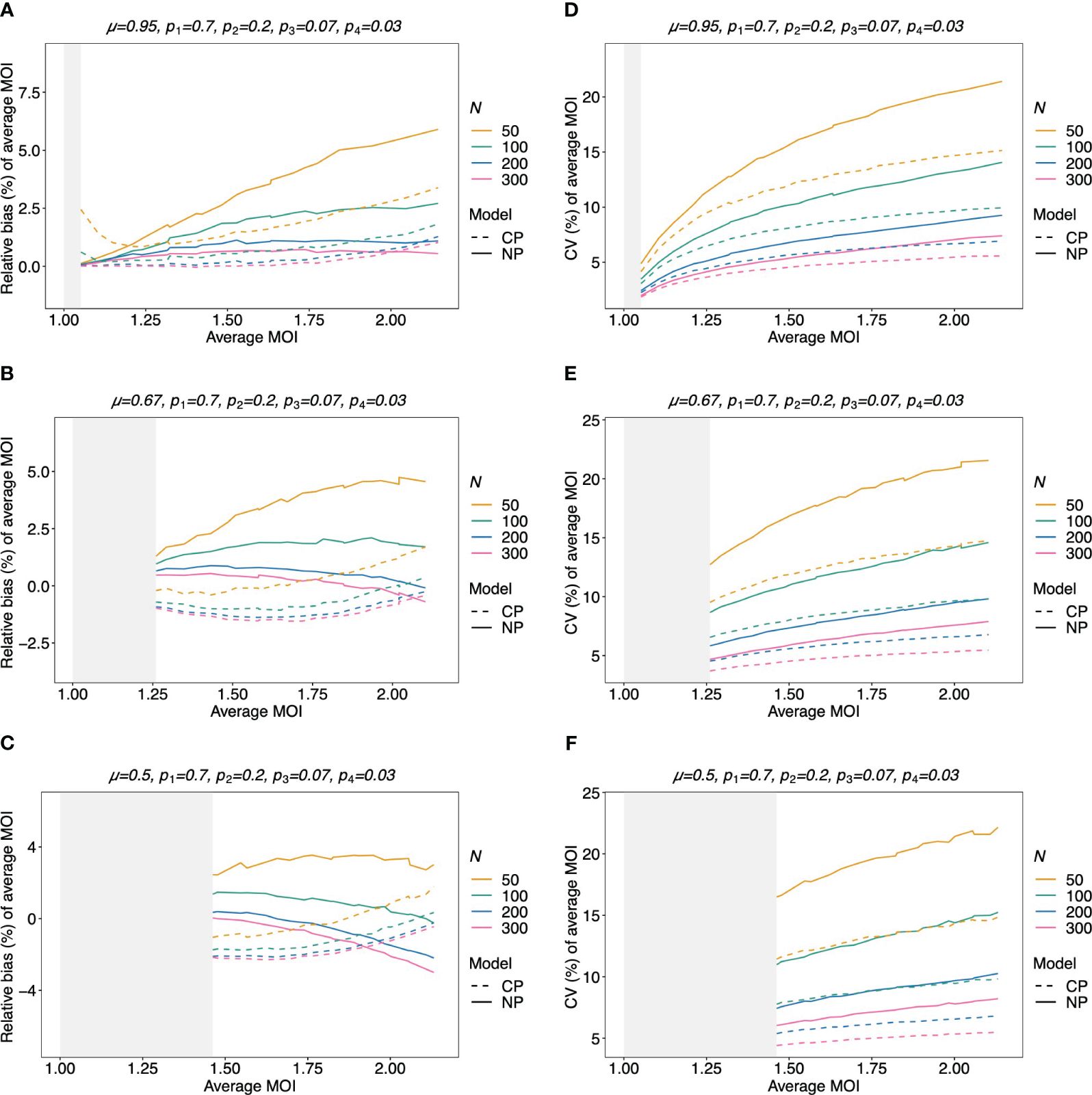
Figure 9 Relative bias and variation of the average MOI for unbalanced lineage frequencies if MOI follows a negative binomial distribution (A–F): see Figure 8 but for an unbalanced lineage frequency distribution (top of each panel).
3.2.5 Variation of the estimates of average MOI
The variation of the estimator of the average MOI (ψ) (Equation 5) measured by the CV increases with increasing true average MOI (Figures 7C, D, 8D–F, and 9D–F). The reason is that the variance of the underlying true MOI distribution is increasing. Moreover, the CV decreases substantially for larger sample sizes (N).
Notably, the CV tends to be smaller for a balanced lineage frequency distribution (cf. Figures 7C, 8D–F, and 9D–F). This is not surprising since the occurrence of different lineages within a sample is more likely for a balanced lineage frequency distribution. Hence, the data tends to harbor more accurate information on the MOI distribution. Particularly, each lineage tends to be represented similarly in the data, thereby reducing the variability of the data. The CV is insensitive to the amount of over-dispersion in the MOI distribution (cf. Figures 7C and 8D–F as well as Figures 7D and 9D–F).
3.2.6 Average MOI estimated by the non-parametric model vs. the conditional Poisson model
Assuming that MOI follows a conditional Poisson distribution, the non-parametric model performs similarly as the conditional Poisson model in terms of bias and variance (i.e., the correct model in this case; cf. Figure 7). However, the variance of the conditional Poisson model tends to be slightly lower than that of the non-parametric model, particularly for unbalanced frequency distributions. However, the differences vanish with increasing sample size. For small and large true average MOI values, the bias of the estimates is lower for the non-parametric model (Figures 7A, B). The same holds true if the true MOI distribution is slightly over-dispersed (Figures 8A, 9A). For highly over-dispersed MOI distributions, the non-parametric model still has a similar variance as the Poisson model, but bias behaves differently. For intermediate average MOI, the Poisson model tends to underestimate the true parameter, with the undesirable property of higher bias for larger sample sizes. For larger average MOI, the Poisson model tends to overestimate the true parameter by roughly the same amount by which the non-parametric model underestimates this parameter (Figures 8B, C and 9B, C).
3.3 Data application
In this section, we apply the non-parametric model introduced here and the alternative Poisson model to three empirical data sets from Cameroon, Kenya, and Venezuela collected during drug resistance studies. The data from Cameroon is described in McCollum et al. (2007) and consists of N = 166 P. falciparum samples collected in Yaoundé between 2001 and 2002. The samples were collected randomly from patients older than 12 years of age at the Nlongkak Catholic missionary dispensary in Yaoundé, Cameroon. The data contains information on 14 neutral microsatellite markers on chromosomes 2 and 3 (for details, see McCollum et al., 2008). At that time, the sampling location was an area of intense and perennial transmission. Although the data consists of random samples, the sampling point and inclusion criteria render the population rather homogeneous. Given the results from the numerical investigations, a good agreement between the two alternative statistical models is expected.
The data set from Kenya is described in McCollum et al. (2012). It contains molecular information from nine neutral microsatellite markers at chromosomes 2 and 3 from N = 43 P. falciparum positive samples collected in Asembo Bay, Kenya, a holoendemic P. falciparum transmission region across 15 villages between April 1992 and March 1993 (see McCollum et al., 2012). Although we would expect transmission to be heterogeneous in this setting because of the small sample size, it is expected that the Poisson model performs similar or even slightly better than the non-parametric model.
The data from Venezuela consists of N = 97 samples collected from 2003 to 2004 in Sifontes municipality in Bolivar State, Venezuela and is described in McCollum et al. (2007). The study area has a population size below 40,000 then and was the epicenter of multi-drug resistance in Venezuela, which accounted for a large proportion of malaria infections in Venezuela (McCollum et al., 2007). However, at the time the samples were collected, the study area was an area of low transmission. Here we included five microsatellite markers, namely, those from the original data that showed evidence of super-infections in at least one sample. Given the low transmission intensity in combination with the sample size (cf. Figures 7A, B), we expect the non-parametric model and the Poisson model to give very similar results.
The maximum likelihood estimate for the MOI distribution and allele frequency distributions were calculated for each molecular marker separately with the non-parametric model and the conditional Poisson model of (Hill and Babiker, 1995; Schneider and Escalante, 2014). These estimates were used as plug-ins to calculate estimates for the average MOI and heterozygosity. These estimates are reported in Figure 10 alongside 95% bootstrap confidence intervals (see Efron and Tibshirani, 1994).
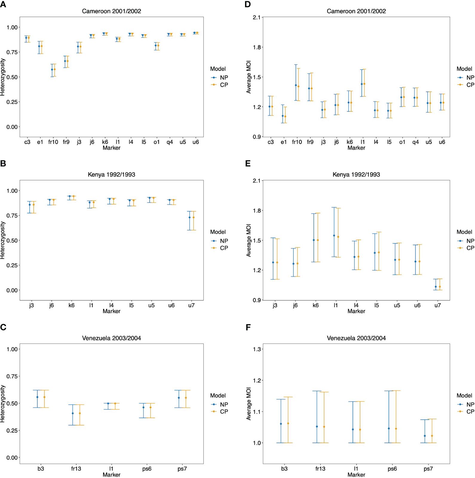
Figure 10 Data application: Shown are the estimated heterozygosity (A, B) and average MOI (C, D) by the non-parametric model (NP) and the conditional Poisson model (CP) with 95% bootstrap CIs for each molecular marker in the data set from Cameroon (A, D), Kenya (B, E), and Venezuela (C, F).
As expected from the above-mentioned considerations and seen from Figure 10, both methods yield very similar results. There is a tendency for the non-parametric model to have slightly lower point estimates of average MOI, particularly for the data set from Kenya, which has a small sample size. This observation is not surprising given the numerical investigations reported above. There are hardly any differences in the estimates of heterozygosity.
Note that the bootstrap confidence intervals do not have satisfying properties, particularly for the data from Venezuela (which hardly has indications of super-infections) and marker u7 in the Kenya data (which also hardly has indications of super-infections). Specifically, the lower confidence points are at 1, which is the minimum possible MOI value. The reason is that the bootstrap frequently repeats samples that have no signs of super-infections, such that the average MOI is estimated to be 1 by both methods. Hence, the nominal coverage of the lower confidence point does not coincide with the actual coverage. This can be resolved by using bias-corrected and accelerated bootstrap confidence intervals or profile-likelihood confidence intervals (cf. Schneider and Escalante, 2014).
4 Discussion
Estimating the multiplicity of infection (MOI) became popular in malaria molecular surveillance. Ad hoc methods are generally biased and have undesirable statistical properties. Methods based on probabilistic models are often based on similar assumptions. A popular assumption in many models is that MOI follows a Poisson distribution. This corresponds to the assumption that infectious events are rare and independent. (Remember, MOI is defined here as the number of super-infections within one disease episode.) Because there is empirical evidence that mosquito biting rates are over-dispersed, the Poisson assumption is challenged.
Here we explored the most flexible alternative, namely, the situation where no parametric assumption about the distribution of MOI is made (except that a maximum MOI exists). Note that the statistical model itself makes a number of simplifying assumptions. First, the duration of how long individuals are infected is not considered. Rather, it is assumed that super-infections occur within a short period of time, such that all variants which were successfully transmitted to a host, reach sufficient frequencies in the infection to be detectable by PCR. Thus, super-infections which do not contribute to the clinical pathogenesis of an infection are ignored. Furthermore, it is assumed that molecular assays have perfect sensitivity and specificity for all relevant lineages in an infection. Notably, the statistical model can be extended to account for missing information (imperfect sensitivity) as in Hashemi and Schneider (2024) (for the Poisson model); however, if all samples contain molecular information (i.e., no sample with missing data), the extended model reduces to the present one. More alternatives can be found in Okell et al. (2017). Extending the model to include imperfect specificity, i.e., including erroneously detected variants, is more challenging. A model that yields appropriate estimates is the one given by Plucinski et al. (2015). However, it is designed to distinguish recrudescence of reinfections and hence requires paired samples (i.e., two or more sample points for at least some patients). Furthermore, it is assumed that the molecular assays used can only provide absence/presence data but cannot quantify the relative abundance of lineages within an infection.
Given this framework, the resulting non-parametric model is more complicated than the corresponding Poisson model (cf. Schneider and Escalante, 2014), which falls into the class of exponential families (Hashemi and Schneider, 2024). This implies the usual desirable properties of maximum likelihood estimators for the Poisson model (existence and uniqueness of the MLE, efficiency, and consistency, cf. Hashemi and Schneider, 2024). Unfortunately, the non-parametric model is no longer within an exponential family and there is no proof for the same desirable theoretical properties. However, our numerical investigations suggest that they hold. In the case of the Poisson model, the MLE has an intuitive interpretation. Namely, the MLE is the parameter choice for which the empirical prevalences coincide with the expected prevalences. Moreover, the empirical prevalences form a sufficient statistic for the parameter estimation. For the non-parametric model, this interpretation is lost and the prevalences no longer form a sufficient statistic. In fact, the model used more information, namely not just how often lineages occur in infections but also in which configuration they are observed. As for the Poisson model, there exists no closed solution for the MLE of the non-parametric model, and it has to be derived numerically. For this purpose, the EM algorithm was employed here. It is a numerically stable and efficient algorithm to derive the MLE.
Notably, the non-parametric model also has certain advantages compared to the Poisson model. If the data lies on the boundary of the closed convex hull of the admissible sample space (when rewritten as a natural exponential family), the MLE of the Poisson model is degenerate (or does not exist; Hashemi and Schneider, 2023). This corresponds to the cases where only a single lineage is detected in every sample (i.e., no evidence of super-infections), or if one lineage is observed in all samples. In such a situation, an MLE is still numerically found for the non-parametric model.
The performance of the non-parametric estimator is comparably good to that of the Poisson model even if the true MOI distribution is well approximated by a Poisson distribution. Despite the Poisson model being the true model for low true MOI, the non-parametric model yields less biased estimates of this parameter. This is also true for high average MOI, at least for a sufficiently large sample size. Moreover, if the true MOI distribution is highly over-dispersed, the non-parametric estimator is preferential. Irrespective of the differences, the results obtained by both models for the empirical examples from Cameroon, Kenya, and Venezuela are very similar. This and the fact that the differences between the estimators are small suggests that there is no need to drop the Poisson assumption, except for extreme parameters or in cases, in which there is clear evidence that the Poisson assumption is unjustified. Therefore, as a recommendation, it seems appropriate to use the non-parametric model in areas of low transmission, particularly, if transmission is highly heterogeneous. In such situations, the Poisson model is highly sensitive to outliers (Schneider, 2018). Areas of low transmission are becoming increasingly important with the ongoing malaria eradication efforts to decrease the global malaria burden by 90% and eradicate the disease in at least 35 countries by 2023 (World Health Organization, 2021). However, in the empirical example from Venezuela, at a time of low transmission, both methods yielded comparable results. In the example, this was due to the relatively large sample size (N = 97). In practice, molecular surveillance data might not always appropriately reflect the heterogeneity in transmission but is rather conducted in homogeneous populations. This renders the Poisson model to be sufficiently accurate.
The results here suggest that the non-parametric approach to estimating MOI is comparably good as the Poisson model. A particularly convenient property of the Poisson distribution is that it is characterized by a single parameter. This is no longer true for the non-parametric model, where the complete probability mass function of MOI needs to be estimated. Although there are many other parametric alternatives to the Poisson model, every other meaningful distribution is characterized by more than a single parameter. Moreover, from the structure outlined in Tsoungui Obama and Schneider (2022), such alternatives also do not retain the desirable properties of the Poisson model.
Given the data, i.e., the absence and presence of alleles in samples, the non-parametric model, is the most flexible assumption for MOI, since it does not require a certain distribution. In principle, the model should be able to approximate any parametric distribution, such as the conditional Poisson or conditional negative binomial distributions. Given that the non-parametric model does not clearly outperform the Poisson model implies that the latter already utilizes the information of data effectively, and any other model assumptions regarding over-dispersion (e.g., assuming a negative binomial distribution) will not outperform the Poisson model either. However, the statistical model can be extended to include further information in addition to the original data—for instance, one could extend the non-parametric model to account for patient-specific risks (e.g., one could group patients into different risk strata based on patient queries determining the risk of exposure, such as the use of bed nets, indoor residual spraying, window screens, etc., or recent malaria cases within the household). In the case of the Poisson model, it could be extended to estimate different MOI parameters for each stratum (risk group). Notably, such information has to be collected in addition to molecular data. In any case, our results suggest that, unless transmission is very heterogeneous, it is not necessary to extend the non-parametric approach to the case in which multiple genetic markers are studies at the same time as it was done for the Poisson model (e.g. Tsoungui Obama and Schneider, 2022; Obama and Schneider, 2023).
In summary, our results suggest that the non-parametric model to estimate MOI and lineage frequencies from single molecular markers (e.g., microsatellites, SNPs, and micro-haplotypes) introduced here is a valid approach. An implementation of the method as an R script is available in the Supplementary Materials and at GitHub https://github.com/Maths-against-Malaria/Non-parametric-MOI-estimation. Clearly, it is possible to extend the non-parametric model to more complex genetic architectures than a single molecular marker following the methodology in Tsoungui Obama and Schneider (2022).
Data availability statement
The original contributions presented in the study are included in the article/Supplementary Material. Further inquiries can be directed to the corresponding author.
Author contributions
LK: Conceptualization, Data curation, Formal analysis, Investigation, Methodology, Software, Visualization, Writing – original draft, Writing – review & editing. KS: Conceptualization, Formal analysis, Funding acquisition, Investigation, Methodology, Project administration, Resources, Software, Supervision, Validation, Visualization, Writing – original draft, Writing – review & editing.
Funding
The author(s) declare financial support was received for the research, authorship, and/or publication of this article. This work was also supported by grants of the German Academic Exchange (DAAD; https://www.daad.de/de/; Project-ID 57417782, Project-ID: 57599539), and the Federal Ministry of Education and Research (BMBF) and the DLR (Project-ID 01DQ20002; https://www.bmbf.de/; https://www.dlr.de/).
Acknowledgments
The authors want to thank Andrea M. McCollum, Dr. Ananias Escalante, and Dr. Venkatachalam (Kumar) Udhayakumar for sharing the data sets from Cameroon, Kenya, and Venezuela. The constructive comments of two reviewers are gratefully acknowledged.
Conflict of interest
The authors declare that the research was conducted in the absence of any commercial or financial relationships that could be construed as a potential conflict of interest.
Publisher’s note
All claims expressed in this article are solely those of the authors and do not necessarily represent those of their affiliated organizations, or those of the publisher, the editors and the reviewers. Any product that may be evaluated in this article, or claim that may be made by its manufacturer, is not guaranteed or endorsed by the publisher.
Supplementary material
The Supplementary Material for this article can be found online at: https://www.frontiersin.org/articles/10.3389/fmala.2024.1363981/full#supplementary-material.
References
Adamidis K. (1999). Theory & methods: An em algorithm for estimating negative binomial parameters. Aust. New Z. J. Stat. 41, 213–221. doi: 10.1111/1467-842X.00075
Alizon S., de Roode J. C., Michalakis Y. (2013). Multiple infections and the evolution of virulence. Ecol. Lett. 16, 556–567. doi: 10.1111/ele.12076
Bandara U., Gill R., Mitra R. (2019). On computing maximum likelihood estimates for the negative binomial distribution. Stat Probability Lett. 148, 54–58. doi: 10.1016/j.spl.2019.01.009
Chang H. H., Worby C. J., Yeka A., Nankabirwa J., Kamya M. R., Staedke S. G., et al. (2017). THE REAL McCOIL: A method for the concurrent estimation of the complexity of infection and SNP allele frequency for malaria parasites. PloS Comput. Biol. 13, 1–18. doi: 10.1371/journal.pcbi.1005348
Couvreur C. (1997). “The em algorithm: A guided tour,” in Kárný M., Warwick K. (eds) Computer intensive methods in control and signal processing (Birkhäuser, Boston, MA). doi: 10.1007/978-1-4612-1996-5_12
Dia A., Cheeseman I. H. (2021). Single-cell genome sequencing of protozoan parasites. Trends Parasitol. 37, 803–814. doi: 10.1016/j.pt.2021.05.013
Efron B., Tibshirani R. J. (1994). An introduction to the bootstrap (1st ed.) (Chapman and Hall/CRC). doi: 10.1201/9780429246593
Galinsky K., Valim C., Salmier A., de Thoisy B., Musset L., Legrand E., et al. (2015). COIL: a methodology for evaluating malarial complexity of infection using likelihood from single nucleotide polymorphism data. Malaria J. 14, 4. doi: 10.1186/1475-2875-14-4
Geiger C., Compaore G., Coulibaly B., Sie A., Dittmer M., Sanchez C., et al. (2014). Substantial increase in mutations in the genes pfdhfr and pfdhps puts sulphadoxine–pyrimethamine-based intermittent preventive treatment for malaria at risk in Burkina Faso. Trop. Med. Int. Health. 19, 690–697. doi: 10.1111/tmi.12305
Guelbeogo W. M., Gonc¸alves B. P., Grignard L., Bradley J., Serme S. S., Hellewell J., et al. (2018). Variation in natural exposure to anopheles mosquitoes and its effects on malaria transmission. Elife 7, e32625. doi: 10.7554/eLife.32625
Gurarie D., McKenzie F. E. (2006). Dynamics of immune response and drug resistance in malaria infection. Malaria J. 5, 86. doi: 10.1186/1475-2875-5-86
Hashemi M., Schneider K. A. (2021). Bias-corrected maximum-likelihood estimation of multiplicity of infection and lineage frequencies. PloS One. 16, e0261889. doi: 10.1371/journal.pone.0261889
Hashemi M., Schneider K. A. (2023). Estimating multiplicity of infection, allele frequencies, and prevalences accounting for incomplete data. bioRxiv. doi: 10.1101/2023.06.01.543300
Hashemi M., Schneider K. A. (2024). Estimating multiplicity of infection, allele frequencies, and prevalences accounting for incomplete data. PloS One. 19, 1–35. doi: 10.1371/journal.pone.0287161
Hastings I. M., Watkins W. M. (2005). Intensity of malaria transmission and the evolution of drug resistance. Acta tropica 94, 218–229. doi: 10.1016/j.actatropica.2005.04.003
Hill W. G., Babiker H. A. (1995). Estimation of numbers of malaria clones in blood samples. Proc. R. Soc. London Ser. B: Biol. Sci. 262, 249–257. doi: 10.1098/rspb.1995.0203
Irvine M. A., Kazura J. W., Hollingsworth T. D., Reimer L. J. (2018). Understanding heterogeneities in mosquitobite exposure and infection distributions for the elimination of lymphatic filariasis. Proc. R. Soc. B: Biol. Sci. 285, 20172253. doi: 10.1098/rspb.2017.2253
Li X., Foulkes A. S., Yucel R. M., Rich S. M. (2007). An expectation maximization approach to estimate malaria haplotype frequencies in multiply infected children. Stat. Appl. Genet. Mol. Biol. 6 Article33, 1-19. doi: 10.2202/1544-6115.1321
Lloyd-Smith J. O. (2007). Maximum likelihood estimation of the negative binomial dispersion parameter for highly overdispersed data, with applications to infectious diseases. PloS One. 2, e180. doi: 10.1371/journal.pone.0000180
McCollum A. M., Basco L. K., Tahar R., Udhayakumar V., Escalante A. A. (2008). Hitchhiking and selective sweeps of plasmodium falciparum sulfadoxine and pyrimethamine resistance alleles in a population from central africa. Antimicrob. Agents Chemother. 52, 4089–4097. doi: 10.1128/AAC.00623-08
McCollum A. M., Mueller K., Villegas L., Udhayakumar V., Escalante A. A. (2007). Common origin and fixation of Plasmodium falciparum dhfr and dhps mutations associated with sulfadoxine-pyrimethamine resistance in a low-transmission area in South America. Antimicrobial Agents chemotherapy 51, 2085–2091. doi: 10.1128/AAC.01228-06
McCollum A. M., Schneider K. A., Griffing S. M., Zhou Z., Kariuki S., Ter-Kuile F., et al. (2012). Differences in selective pressure on dhps and dhfr drug resistant mutations in western Kenya. Malaria J. 11, 1–14. doi: 10.1186/1475-2875-11-77
Neafsey D. E., Taylor A. R., MacInnis B. L. (2021). Advances and opportunities in malaria population genomics. Nat. Rev. Genet. 22, 502–517. doi: 10.1038/s41576-021-00349-5
Ng S. K., Krishnan T., McLachlan G. J. (2012). “The em algorithm,” Handbook of computational statistics: concepts and methods, 139–172. edited by Gentle J. E., Hardle W. K., Mori Y. Berlin & New York: Springer. doi: 10.1007/978-3-642-21551-3__6
Nkhoma S. C., Nair S., Cheeseman I. H., Rohr-Allegrini C., Singlam S., Nosten F., et al. (2012). Close kinship within multiple-genotype malaria parasite infections. Proc. Biol. Sci. 279, 2589–2598. doi: 10.1098/rspb.2012.0113
Nkhoma S. C., Trevino S. G., Gorena K. M., Nair S., Khoswe S., Jett C., et al. (2020). Co-transmission of related malaria parasite lineages shapes within-host parasite diversity. Cell Host Microbe. 27, 93–103.e4. doi: 10.1016/j.chom.2019.12.001
Noor A. M., Kinyoki D. K., Mundia C. W., Kabaria C. W., Mutua J. W., Alegana V. A., et al. (2014). The changing risk of plasmodium falciparum malaria infection in africa: 2000–10: a spatial and temporal analysis of transmission intensity. Lancet 383, 1739–1747. doi: 10.1016/S0140-6736(13)62566-0
Obama H. C. J. T., Schneider K. A. (2023). Estimating multiplicity of infection, haplotype frequencies, and linkage disequilibria from multi-allelic markers for molecular disease surveillance. bioRxiv. doi: 10.1101/2023.08.29.555251
Okell L. C., Griffin J. T., Roper C. (2017). Mapping sulphadoxine-pyrimethamine-resistant plasmodium falciparum malaria in infected humans and in parasite populations in africa. Sci. Rep. 7, 7389. doi: 10.1038/s41598-017-06708-9
Pacheco M. A., Forero-Peña D. A., Schneider K. A., Chavero M., Gamardo A., Figuera L., et al. (2020). Malaria in Venezuela: changes in the complexity of infection reflects the increment in transmission intensity. Malaria J. 19, 176. doi: 10.1186/s12936-020-03247-z
Pacheco M. A., Lopez-Perez M., Vallejo A. F., Herrera S., Arévalo-Herrera M., Escalante A. A. (2016). Multiplicity of infection and disease severity in plasmodium vivax. PloS Negl. Trop. Dis. 10, e0004355. doi: 10.1371/journal.pntd.0004355
Piegorsch W. W. (1990). Maximum likelihood estimation for the negative binomial dispersion parameter. Biometrics, 46(3), 863–867. doi: 10.2307/2532104
Plucinski M. M., Morton L., Bushman M., Dimbu P. R., Udhayakumar V. (2015). Robust algorithm for systematic classification of malaria late treatment failures as recrudescence or reinfection using microsatellite genotyping. Antimicrob. Agents Chemother. 59, 6096–6100. doi: 10.1128/AAC.00072-15
R Core Team (2023). “R: A language and environment for statistical computing,” in R foundation for statistical computing (Vienna, Austria).
Read A. F., Taylor L. H. (2001). The ecology of genetically diverse infections. Science 292, 1099–1102. doi: 10.1126/science.1059410
Saha K., Paul S. (2005). Bias-corrected maximum likelihood estimator of the negative binomial dispersion parameter. Biometrics 61, 179–185. doi: 10.1111/j.0006-341X.2005.030833.x
Schneider K. A. (2018). Large and finite sample properties of a maximum-likelihood estimator for multiplicity of infection. PloS One. 13, e0194148. doi: 10.1371/journal.pone.0194148
Schneider K. A. (2021). Charles darwin meets ronald ross: A population-genetic framework for the evolutionary dynamics of malaria Vol. 6 (Cham: Springer International Publishing), 149–191. doi: 10.1007/978–3-030–50826-56
Schneider K. A., Escalante A. A. (2014). A likelihood approach to estimate the number of co-infections. PloS One. 9, e97899. doi: 10.1371/journal.pone.0097899
Schneider K. A., Kim Y. (2010). An analytical model for genetic hitchhiking in the evolution of antimalarial drug resistance. Theor. Population Biol. 78, 93–108. doi: 10.1016/j.tpb.2010.06.005
Schneider K. A., Salas C. J. (2022). Evolutionary genetics of malaria. Front. Genet. 13. doi: 10.3389/fgene.2022.1030463
Schneider K. A., Tsoungui Obama H. C. J., Kamanga G., Kayanula L., Adil Mahmoud Yousif N. (2022). The many definitions of multiplicity of infection. Front. Epidemiol., 2, 961593. doi: 10.3389/fepid.2022.961593
Sinha A., Kar S., Deora N., Dash M., Tiwari A., Kori L., et al. (2023). India-embo lecture course: understanding malaria from molecular epidemiology, population genetics, and evolutionary perspectives. Trends Parasitol. 39, 307–313. doi: 10.1016/j.pt.2023.02.010
Tsoungui Obama H. C. J., Schneider K. A. (2022). A maximum-likelihood method to estimate haplotype frequencies and prevalence alongside multiplicity of infection from snp data. Front. Epidemiol. 2, 943625. doi: 10.3389/fepid.2022.943625
Wong W., Wenger E. A., Hartl D. L., Wirth D. F. (2018). Modeling the genetic relatedness of Plasmodium falciparum parasites following meiotic recombination and cotransmission. PloS Comput. Biol. 14, e1005923. doi: 10.1371/journal.pcbi.1005923
World Health Organization (2022). Global genomic surveillance strategy for pathogens with pandemic and epidemic potential, 2022–2032 Vol. VI (Geneva: World Health Organization), 21.
Keywords: malaria, complexity of infection, molecular surveillance, drug resistance, prevalence, transmission intensities, superinfection, co-infection
Citation: Kayanula L and Schneider KA (2024) A non-parametric approach to estimate multiplicity of infection and pathogen haplotype frequencies. Front. Malar. 2:1363981. doi: 10.3389/fmala.2024.1363981
Received: 31 December 2023; Accepted: 07 May 2024;
Published: 18 July 2024.
Edited by:
Sarah Reece, University of Edinburgh, United KingdomReviewed by:
Megan Greischar, Cornell University, United StatesLucy Okell, Imperial College London, United Kingdom
Copyright © 2024 Kayanula and Schneider. This is an open-access article distributed under the terms of the Creative Commons Attribution License (CC BY). The use, distribution or reproduction in other forums is permitted, provided the original author(s) and the copyright owner(s) are credited and that the original publication in this journal is cited, in accordance with accepted academic practice. No use, distribution or reproduction is permitted which does not comply with these terms.
*Correspondence: Loyce Kayanula, bGtheWFudWxAaHMtbWl0dHdlaWRhLmRl