1
Neuroscience Department, The Mount Sinai School of Medicine, New York, NY, USA
2
Laboratory of Biophysics, The Rockefeller University, New York, NY, USA
Although all brain functions require coordinated activity of many neurons, it has been difficult to estimate the amount of information carried by a population of spiking neurons. We present here a Fourier-based method for estimating the information delivery rate from a population of neurons, which allows us to measure the redundancy of information within and between functional neuronal classes. We illustrate the use of the method on some artificial spike trains and on simultaneous recordings from a small population of neurons from the lateral geniculate nucleus of an anesthetized macaque monkey.
The brain processes information, and it is therefore natural to estimate the amount of information that a neuron transmits to its targets. In the past, several methods that derive such estimates from the firing pattern (Optican and Richmond, 1987
; Richmond and Optican, 1987
; Richmond et al., 1987
; Bialek et al., 1991
; Rieke et al., 1997
; Strong et al., 1998
; Brenner et al., 2000
) or membrane potential (Borst and Theunissen, 1999
; DiCaprio, 2004
) of individual neurons have been used. The information from spike trains was estimated by calculating the entropy associated with the various temporal patterns of spike discharge, using Shannon’s formula (Shannon and Weaver, 1949
).
Since all brain functions involve many neurons, it is desirable to provide similar information estimates for a neuronal population (Knight, 1972
). To simply add up the information amounts from individual neurons in the population would be valid only if the neurons were all independent of one another, an assumption that usually is incorrect (see, for example, Zohary et al., 1994
; Bair et al., 2001
; Pillow et al., 2008
). Approaches like the Direct Method (Strong et al., 1998
) are impractical for a population, because the multi-dimensional space occupied by many spike trains can be sampled only sparsely by most neurophysiological experiments. Calculating the information carried by a population of many neurons thus has remained a challenge (Brown et al., 2004
; Quiroga and Panzeri, 2009
). At the same time, the need for such estimates has become increasingly urgent, since the technology of recording simultaneously from many neurons has become much more affordable and wide-spread, and data from such recordings are becoming common.
We describe here a method that estimates the amount of information carried by a population of spiking neurons, and demonstrate its use, first with simulated data and then with data recorded from the lateral geniculate nucleus (LGN) of an anesthetized macaque monkey.
Surgical Preparation
The experimental methods were similar to those used in our lab in the past (Uglesich et al., 2009
). Housing, surgical and recording procedures were in accordance with the National Institutes of Health guidelines and the Mount Sinai School of Medicine Institutional Animal Care and Use Committee. Adult macaque monkeys were anesthetized initially with an intramuscular injection of xylazine (Rompun, 2 mg/kg) followed by ketamine hydrochloride (Ketaset, 10 mg/kg), and then given propofol (Diprivan) as needed during surgery. Local anesthetic (xylocaine) was used profusely during surgery, and was used to infiltrate the areas around the ears. Anesthesia was maintained with a mixture of propofol (4 mg/kg-hr) and sufentanil (0.05 μg/kg-hr), which was given intravenously (IV) during the experiment. Propofol anesthesia has been shown to cause no changes in blood flow in the occipital cortex (Fiset et al., 1999
), and appears to be optimal for brain studies. Cannulae were inserted into the femoral veins, the right femoral artery, the bladder, and the trachea. The animal was mounted in a stereotaxic apparatus. Phenylephrine hydrochloride (10%) and atropine sulfate (1%) were applied to the eyes. The corneas were protected with plastic gas-permeable contact lenses, and a 3-mm diameter artificial pupil was placed in front of each eye. The blood pressure, electrocardiogram, and body temperature were measured and kept within the physiological range. Paralysis was produced by an infusion of pancuronium bromide (Norcuron, 0.25 mg/kg-hr), and the animal was artificially respired. The respiration rate and stroke volume were adjusted to produce an end-expiratory value of 3.5–4% CO2 at the exit of the tracheal cannula. Penicillin (750,000 units) and gentamicin sulfate (4 mg) were administered IM to provide antibacterial coverage, and dexamethasone was injected IV to prevent cerebral edema. A continuous IV flow (3–5 ml/kg-hr) of lactated Ringer’s solution with 5% dextrose was maintained throughout the experiment to keep the animal properly hydrated, and the urinary catheter monitored the overall fluid balance. Such preparations are usually stable in our laboratory for more than 96 h. The animal’s heart rate and blood pressure monitored the depth of anesthesia, and signs of distress, such as salivation or increased heart rate, were watched for. If such signs appeared, additional anesthetics were administered immediately.
Visual Stimulation
The eyes were refracted, and correcting lenses focused the eyes for the usual viewing distance of 57 cm. Stimuli were presented monocularly on a video monitor (luminance: 10–50 cd/m2) driven by a VSG 2/5 stimulator (CRS, Cambridge, UK). The monitor was calibrated according to Brainard (1989) and Wandell (1995
). Gamma corrections were made with the VSG software and photometer (OptiCal). Visual stimuli consisted of homogeneous field modulated in luminance according to a pseudo-random naturalistic sequence (van Hateren, 1997
). Eight second segments of the luminance sequences were presented repeatedly 128 times (‘repeats’), alternating with 8 s non-repeating (‘uniques’) segments of the sequence (Reinagel and Reid, 2000
). In addition, we used steady (unmodulated) light screens and dark screens, during which spontaneous activity was recorded.
Electrophysiological Recording
A bundle of 16 stainless steel microwires (25 μ) was inserted into a 22 gauge guard tube, which was inserted into the brain to a depth of 5 mm above the LGN. The microwire electrodes were then advanced slowly (in 1 μ steps) into the LGN, until visual responses to a flashing full field screen were detected. The brain over the LGN was then covered with silicone gel, to stabilize the electrode bundle. Based on the electrode depth, dominant eye sequence and cell properties (Kaplan, 2007
), we are confident that all the electrodes were within the parvocellular layers of the LGN. The receptive fields of the recorded cells covered a relatively small area (∼4° in diameter), which suggests that the electrodes bundle remained relatively compact inside the LGN.
The output of each electrode was amplified, band-pass filtered (0.75–10 kHz), sampled at 40 kHz and stored in a Plexon MAP computer for further analysis.
Data Analysis
Spike sorting
Sorting procedures. The spike trains were first thresholded (SNR ≥5) and sorted using a template-matching algorithm under visual inspection (Offline Sorter, Plexon Inc., Dallas, TX, USA). In most cases, spikes from several neurons recorded by a given electrode could be well-separated by this simple procedure. In more difficult cases, additional procedures (peak- or valley-seeking, or multi-variate t-distributions) (Shoham et al., 2003
) were employed. Once the spikes were sorted, a firing times list was generated for each neuron and used for further data analysis.
Quality assurance. To ensure that all the spikes in a given train were fired by the same neuron, we calculated for each train the interspike interval (ISI) histogram. If we found intervals that were shorter than the refractory period of 2 ms, the spike sorting was repeated to eliminate the misclassified spikes. We ascertained that all the analyzed data came from responsive cells by calculating the coefficients of variation of the peristimulus time histogram bin counts for the responses to the repeated and unique stimuli, and taking the ratio of these two coefficients. Only cells for which that ratio exceeded 1.5 were included in our analysis.
Generation of surrogate data
To test our method we generated synthetic spike trains from a Poisson renewal process, in which the irregularities of neuronal spike times are modeled by a stochastic process whose mathematical properties are well defined. Recent interest and success in modeling a neuron spike-train as an inhomogeneous Poisson process (Pillow et al., 2005
, 2008
; Pillow and Simoncelli, 2006
) led us to that choice.
Firing rates and input. Our modeling necessarily addressed two major features of the laboratory data. The nine real neurons show a range of mean firing rates, from 3.04 impulses per second (ips) to 28.72 ips, which span an order of magnitude. To mimic this, we gave our 12 model cells 12 inputs which consecutively incremented by a factor of 10(1/11), to give firing rates spanning an order of magnitude. The second major feature was that our laboratory neurons evidently received inputs processed in several ways following the original retinal stimulus. To make a simple caricature of this, we drove each of our Poisson model neurons with a separate input that was a weighted mean admixture of two van Hateren-type stimuli. The first was that which we used in the laboratory and the second was the time-reversal of that stimulus. Calling these A and B, the stimuli were of the form S = (1 − x)·A + x · B, where the admixture variable x took on 12 equally spaced values starting with 0 and ending with 1. As shown in Table 1
, the pairs (admixture, mean rate) were chosen in a manner that allowed the whole grouping of model cells to be divided into smoothly changing subsets in different ways, and evenly distributed the range of properties across all cells.

Table 1. Parameters for stimulating the surrogate neurons. Each surrogate neuron was driven by a mixture of two van Hateren inputs, chosen to cover uniformly the range of firing rates and mixture ratios.
Estimation of the information delivered by a subset of neurons
If we have data from numerous parallel spike trains, the familiar Direct method (Strong et al., 1998
) for computing signal information delivered requires an impractical time span of data. As a practical alternative we advance a straightforward multi-cell generalization of a method of information computation from basis-function coefficients.
Shannon has observed (Shannon and Weaver, 1949
, Chapter 4; see also Shannon, 1949
) that the probability structure of a stochastic signal over time may be well approximated in many different ways by various equivalent multivariate distribution density functions of high but finite dimension. He further observed that when some specific scheme is used to characterize both the distribution of signal-plus-noise and the distribution of noise alone, the information quantity one obtains for the signal alone, by taking the difference of the information quantities (commonly called ‘entropies’) evaluated from the two distributions, has a striking invariance property: the value of the signal information is universal, and does not depend on which of numerous possible coordinate systems one has chosen in which to express the multivariate probability density (see extensive bibliography, and discussion, in Rieke et al., 1997
, chapter 3). We will follow Shannon (1949)
, whose choice of orthonormal functions was Fourier normalized sines and cosines, over a fixed, but long, time span T. This choice has the added virtue of lending insight into the frequency structure of the information transfer under study.
Here we outline our approach for obtaining the signal-information rate, or ‘mutual information rate’, transmitted by the simultaneously recorded spikes of a collection of neurons. The mathematical particulars are further elaborated in the Appendix. Following Shannon (1949)
, if one has a data record that spans a time T, it is natural to use the classical method of Fourier analysis to resolve that signal into frequency components, each of which speaks of the information carried by frequencies within a frequency bandwidth of 1/T. If this is repeated for many samples of output, one obtains a distribution of amplitudes within that frequency band. In principle, that probability distribution can be exploited to calculate how many bits would have to be generated per second (the information rate) to describe the information that is being transmitted within that frequency band.
However, part of that information rate represents not useful information but the intrusion of noise. To quantify our overestimate we may repeat the experiment many times without variation of input stimulus, and in principle may employ the same hypothetical means as before to extract the ‘information’, which now more properly may be called ‘noise entropy’. When this number is subtracted from the previous, we obtain the mutual information rate, in bits per second, carried by the spikes recorded from that collection of neurons.
In order to reduce the above idea to practice, we have exploited the following fact (which apparently is not well known nor easily found in the literature): if our response forgets its past history over a correlation time span that is brief compared to the experiment time span, T, then the central limit theorem applies, and our distribution of signal measurements within that narrow bandwidth will follow a Gaussian distribution. If we are making simultaneous recordings from a collection of neurons, their joint probability distribution within that bandwidth will be multivariate Gaussian. A Gaussian with known center of gravity is fully characterized by its variance, and similarly a multivariate Gaussian by its covariance matrix. Such a covariance matrix, which can be estimated directly from the data, carries with it a certain entropy. By calculating the covariance matrices for responses to both unique and repeated stimuli, one can determine the total signal information flowing through each frequency channel for a population of neurons.
To verify that our Gaussian assumption is valid, we have applied to our Fourier-coefficient sample sets two standard statistical tests that correctly identify a sample as Gaussian with 95% accuracy. For our 12 surrogate cells and 9 laboratory LGN cells, the degree of verification across the frequency range for 2560 distribution samples (160 Hz × 8 bins/Hz × 2, with each sine and cosine term sampled 128 times) is shown in Table 2
. Because of its importance, we return to this issue in the Discussion, where further evidence is provided for the Gaussian nature of the underlying distributions.
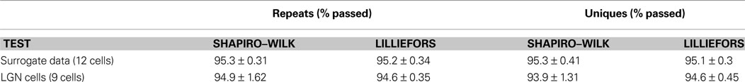
Table 2. The Fourier coefficients for the surrogate and LGN data follow a Gaussian distribution. We sampled the Fourier coefficients 128 times for each of the 2560 sine and cosine terms that we tested for each cell. Each distribution was tested with two standard tests for normality: the Shapiro–Wilk’s test and the Lilliefors test. The percentage of distributions that passed each test at the p < 0.05 significance level was calculated for each cell, and the table gives the mean and standard deviation for the test results.
Analysis of Simulated Spike Trains
Entropy vs temporal frequency
In anticipation of analyzing simultaneous laboratory records of actual neurons, we have created 12 Poisson model neurons with firing rates that overlap those of our laboratory neurons and with inputs as discussed above in Section ‘Materials and Methods’, presented at the same rate (160 Hz) used in the laboratory experiments. Figure 1
shows, for a single simulated cell, the entropy rate per frequency, for responses to unique and repeat stimuli. The entropy from the responses to the unique stimulus (signal plus noise) exceeds that of the responses to the repeated stimulus (noise alone) at low frequencies, and the two curves converge near the monitor’s frame-rate of 160 Hz, beyond which signal-plus-noise is entirely noise. Hence we will terminate the sum in (Eq. A26) at that frequency. The difference between the two curves at any temporal frequency is the mutual information rate at that frequency.
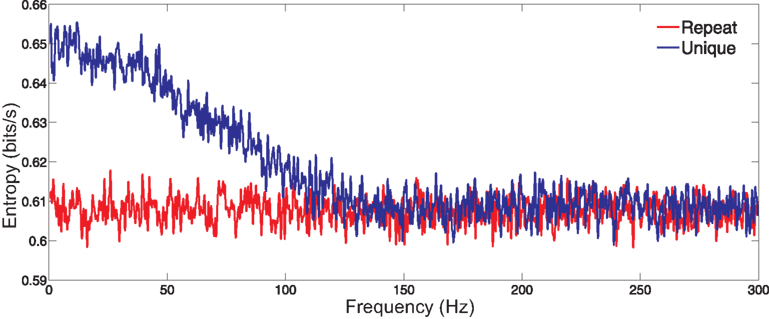
Figure 1. Entropy per frequency conveyed by a single surrogate neuron. The signal-plus-noise entropy (derived from the unique stimuli) is shown in blue, and the noise entropy (from the repeated stimulus) is shown in red. The data shown are typical of data from other cells.
Single cell information
For the 12 model cells, the cumulative sum of information over frequency (Eq. A26) is given in Figure 2
(left frame). We note that all the curves indeed finish their ascent as they approach 160 Hz. More detailed examination shows a feature that is not obvious: the output information rate of a cell reflects its input information rate, and the input information rate of a mixed, weighted mean input is less than that of a pure, unmixed input. This accounts for the observation that the second-fastest cell (cell 11, with a near even mixture) delivers information at only about half the rate of the fastest (cell 12).
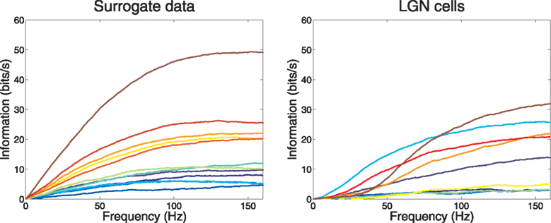
Figure 2. Cumulative information rate vs frequency for 12 surrogate Poisson model neurons and 9 LGN cells. The firing rates of the various neurons in the two groups were similar.
Group information
We turn now to the information rate of a group of cells, firing in parallel in response to related stimuli. We proceed similarly to what is above, but use the multi-cell equation (Eq. A25) and its cumulative sum over frequencies. As a first exercise we start with the slowest-firing surrogate cell and then group it with the next-slowest, next the slowest 3 and so on up to the fastest; the set of cumulative curves we obtain from these groupings are shown in the left frame of Figure 3
. Again we see that the accumulation of information appears to be complete earlier than the frame-rate frequency of 160 Hz.
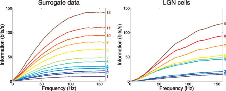
Figure 3. Group information vs frequency for our Poisson model surrogate neurons and 9 LGN cells. The group size is indicated to the right of the cumulative curve for each group. The neurons were ranked according to their firing rate. The first group contained only the slowest firing neuron, and each new group was formed by adding the next ranking cell.
Redundancy and Synergy among Neurons in a Population
Redundancy
The mutual information communicated by a group of cells typically falls below the sum of the mutual information amounts of its constituent members. This leads us to define a measure of information redundancy. The redundancy of a cell with respect to a group of cells can be intuitively described as the proportion of its information already conveyed by other members of the group. For example, if a cell is added to a group of cells and 100% of its information is novel, then it has 0 redundancy. If, on the other hand, the cell brings no new information to the group, then it contains only redundant information, and it therefore has redundancy 1. With this in mind, we define the redundancy of a cell C, after being added to a group G, as:
According to this formula, if all the information of the additional cell appears as added information in the new group, then that cell’s redundancy is zero.
The procedure of information redundancy evaluation is general, and can be applied to the addition of any cell to any group of cells. Thus for the cell groups of Figure 3
, we can evaluate the redundancy of each newly added cell not only upon its addition to the group but also thereafter. This is shown for the 70 resulting redundancies, in Figure 4
(Left).
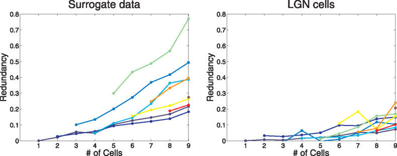
Figure 4. Accumulating redundancy as more cells are added to a population. The cells are added in order of their mean firing rates, starting with the slowest firing cells, with each cell taking its turn as a starting point for a new population.
Synergy
When the total information conveyed by several neurons exceeds the sum of the individual ones, the neurons are synergistic (Gawne and Richmond, 1993
; Schneidman et al., 2003
; Montani et al., 2007
). When this happens, our formula yields a negative redundancy value.
Analysis of Monkey LGN Spike Trains
We now apply the same techniques to simultaneous laboratory recordings of 9 parvocellular cells from the LGN of a macaque monkey, responding to a common full-field naturalistic stimulus (van Hateren, 1997
; Reinagel and Reid, 2000
).
Figure 2
(right frame) shows the single cell cumulative information of these neurons as frequency increases. In two obvious ways their behavior differs from that of the Poisson model neurons. First, at low frequency there is a qualitative difference indicative of initially very small increment, which differs from the Poisson model’s initial linear rise. Second, the real geniculate neurons show a substantial heterogeneity in the shape of their rise curves. For example, the second most informative cell (cell 8), has obtained half its information from frequencies below 40 Hz, while the most informative cell (cell 9) has obtained only 11% of its information from below that frequency.
The right frame of Figure 3
shows for LGN cells the accumulating multineuron group information, while the left frame shows it for the surrogate data.
Redundancy in surrogate and real LGN neurons
Figure 4
(right frame) compares the redundancy over the 9 LGN cells with what was shown for the first 9 Poisson model neurons in Figure 4
(left frame). The pair of sharp features at cells 4 and 7 might be attributed to difficulties in spike separation. Note that the redundancy of real neurons appears to be quite different from that of their Poisson model counterparts: as cluster size increases, real cells manifest a stronger tendency than our simulated neurons to remain non-redundant. This implies that the different LGN neurons are reporting with differences in emphasis on the various temporal features of their common stimulus.
The Validity of the Gaussian Assumption
Our method exploits the theoretical prediction that the distribution of each stochastic Fourier coefficient of our data should be Gaussian. Our evidence supports this prediction. A standard visual check is to normalize a distribution by a Z-score transformation and plot its quantiles against those of a standard Gaussian. If the distribution is likewise Gaussian, the points will fall near a unit-slope straight line through the origin. Figure 5
shows two typical cases, each with 128 points: surrogate data in the left frame and LGN cell data on the right. Both show good qualitative confirmation of the Gaussian assumption.
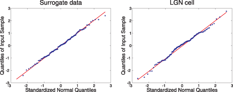
Figure 5. Q–Q plots for the Fourier coefficients of one surrogate cell (#6) and one LGN cell (#4). The data are typical of data from other cells. The fact that the data points hug the y = x line demonstrates the Gaussian nature of the distributions of the Fourier coefficients.
We have proceeded to apply to our numerous Fourier coefficient distributions two standard statistical tests for Gaussian distribution: the Shapiro–Wilk test and the Lilliefors test. Both are designed to confirm that a sample was drawn from a true Gaussian distribution in 95% of cases. Table 2
shows that in almost all cases for both unique and repeat responses of our 12 surrogate and 9 LGN cells our distributions passed both tests at the 95% significance level.
Small Sample Bias
In the extraction of mutual information from spike data, traditional methods suffer from a bias due to the small size of the sample. We checked the Fourier method for such bias by dividing our sets of 128 runs into subsets of 64, 32 and 16 runs. The results for one surrogate cell (number 12) and one LGN cell (number 8) are shown in Figure 6
. These results are typical, and show no clear small-sample bias. We also notice that, for these data, a sample of 64 runs gives a mutual information estimate reliable to better than ±10%. A summary of small-sample bias and estimated reliability for several recent techniques for calculating spike-train mutual information is given by Ince et al. (2009)
(their Figure 1).
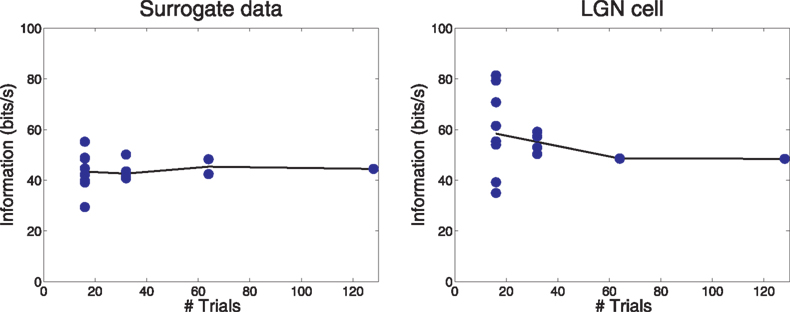
Figure 6. The effect of the number of trials on information calculation. Data are from surrogate cell #12 and LGN cell #8, which were typical of other cells. Solid symbols show the information calculated from individual segments of the record. The solid line connects the medians of the samples. Note the rapid convergence of the information estimates as the number of trials increases.
In addition to the number of data segments, the number of spikes used in estimating the mutual information is also an important factor, and we discus it further at the end of the Appendix.
Summary and Conclusions
We have presented a new method for calculating the amount of information transmitted by a neuronal population, and have applied it to populations of simulated neurons and of monkey LGN neurons. Since the method can be used also to calculate the information transmitted by individual cells, it provides an estimate of the redundancy of information among the members of the population. In addition, the method reveals the temporal frequency bands at which the communicated information resides.
The new method fills a gap in the toolbox of the modern neurophysiologist, who now has the ability to record simultaneously from many neurons. The methodology presented here might permit insights regarding the mutual interactions of neuronal clusters, an area that has been explored less than the behavior of single neurons or whole organisms.
Suppose we have a stochastic numerical data-stream that we will call u(t), and which becomes uncorrelated for two values of t that are separated by a time interval greater than a maximum correlation time-interval t*. That is to say, if t2 − t1 > t*, then u(t2) and u(t1) are independent random variables in the probability sense. Suppose now that in the laboratory, by running the probabilistically identical experiment repeatedly, we gather N realizations (samples) of u(t), the nth of which we will call u(n) (t). Suppose further that we collect each data sample over a time-span T that is large compared to the correlation time interval t*.
We can represent each sample u(n) (t) to whatever accuracy we desire, as a discrete sequence of numbers in the following way. Over the time interval t = 0 to t = T, we choose a set of functions φm(t) that are orthonormal in the sense that they have the property:
Then u(n) (t) may be represented as a weighted sum of these basis functions:

where the weighting coefficients  may be evaluated from the data by,
may be evaluated from the data by,
This claim can be verified if we substitute (Eq. A2) into (Eq. A3) and then use (Eq. A1) to evaluate the integral. Here our choice of the φm (t) will be the conventional normalized sinusoids:
It is a straightforward exercise to show that these functions have the property required by (Eq. A1).
Now let us see what follows from T >> t*. Divide the full time-span T into K sub-intervals by defining the division times:

and define the integrals over shorter sub-intervals:
from which (Eq. A3) tells us that the Fourier coefficient  is given by,
is given by,
But we note that the measure of the support of the integral (Eq. A7) is smaller than that of (Eq. A6) by the ratio t*/((T/K) − t*) , and if we can pick T long enough, we can make that ratio as close to zero as we choose. So the second sum in (Eq. A8) is negligible in the limit. But now note that, because they are all separated from each other by a correlation time, the individual terms in the first sum are realizations of independent random variables. If the distribution of an individual term in the sum is constrained in any one of a number of non-pathological ways, and if there are a sufficient number of members in the sum, then the central limit theorem states that the distribution of the sum approaches a Gaussian.
In the more general case, where we have several simultaneous correlated numerical data-streams, the argument runs exactly the same way. If, for many repeated samples, at a particular frequency we compute the Fourier coefficient for each, to estimate a multivariate probability density, then from a long enough time span, by the multivariate central limit theorem that density will approach a multivariate Gaussian. Simply because the notation is easier, we elaborate the univariate case first.
Specializing, for cell response we use the spike train itself, expressed as a sequence of δ-functions, so for the rth realization u(r) (t) of the stochastic spike-train variable u(t), we have:

where t(r)n is the time of the nth spike of the rth realization, and Nr is the total number of spikes that the cell under discussion fires in that realization.
Substituting this and also (Eq. A4) into (Eq. A3) we see that the integral may be performed at once. In the cosine case of (Eq. A4) it is,

Before proceeding further we look back at Eq. A8 and note that, because a cosine is bounded between +1 and −1, every term in the sums of (Eq. A8) is bounded in absolute value by  times the number of spikes in that sub-interval. As real biology will not deliver a cluster of spikes overwhelmingly more numerous than the local mean rate would estimate, the distribution of each term in the stochastic sum cannot be heavy-tailed, and we may trust the central limit theorem.
times the number of spikes in that sub-interval. As real biology will not deliver a cluster of spikes overwhelmingly more numerous than the local mean rate would estimate, the distribution of each term in the stochastic sum cannot be heavy-tailed, and we may trust the central limit theorem.Thus we may estimate that the probability density function for the stochastic Fourier coefficient variable um is of the form,

where,
The right-hand-most expressions in (Eq. A12), (Eq. A13) testify that  and Vm can be estimated directly from the available laboratory data.
and Vm can be estimated directly from the available laboratory data.What is the information content carried by the Gaussian (Eq. A11)? The relevant integral may be performed analytically:

For a signal with finite forgetting-time the stochastic Fourier coefficients (Eq. A10) at different frequencies are statistically independent of one another, so that the signal’s full multivariate probability distribution in terms of Fourier coefficients is given by,

It is easily shown that if a multivariate distribution is the product of underlying univariate building blocks, then its information content is the sum of the information of its components, whence

Observing (Eq. A13) we note that this can be evaluated from available laboratory data.
Generalization of the information rate calculation to the case of multiple neurons is conceptually straightforward but notationally messy due to additional subscripts. The rth realization’s spike train from the qth neuron (out of a total of Q neurons) may be defined as a function of time  just as in (Eq. A9) above, and from our orthonormal set of sines and cosines we may find the Fourier coefficient
  This number is a realization drawn from an ensemble whose multivariate probability density function we may call:
just as in (Eq. A9) above, and from our orthonormal set of sines and cosines we may find the Fourier coefficient This number is a realization drawn from an ensemble whose multivariate probability density function we may call:
This density defines a vector center of gravity  whose Q components are of the form:
whose Q components are of the form:
and similarly it defines a covariance matrix Vm whose (q,s)th matrix element is given by,
This covariance matrix has a matrix inverse Am:

Clearly (Eq. A18) and (Eq. A19) are the multivariate generalizations of (Eq. A12) and (Eq. A13) above. The central limit theorem’s multivariate Gaussian generalization of (Eq. A11) is,
This expression becomes less intimidating in new coordinates Z(q) with new origin located at the center of gravity and orthogonally turned to diagonalize the covariance matrix (Eq. A19). We need not actually undertake this task. Call the eigenvalues of the covariance matrix

Under the contemplated diagonalizing transformation, the double sum in the exponent collapses to a single sum of squared terms, and in the new coordinates pm becomes,

a form that is familiar from (Eq. A15) above. Its corresponding information is the sum of those of the individual terms of the product and is
Shannon (1949
, chapter 4), in a formally rather analogous context, has noted that much care is needed in the evaluation of expressions similar to (Eq. A24) from laboratory data. The problem arises here if the eigenvalues approach zero (and their logarithms tend to −∞) before the sum is completed. However, the information in signal-plus-noise in the mth coefficient, expressed by (Eq. A24) is not of comparable interest to the information from signal alone. With some caution, this signal-alone information contribution may be obtained by subtracting from (Eq. A24) a similar expression for noise alone, taken from additional laboratory data in which the same stimulus was presented repeatedly. If we use ‘μ’ to annotate the eigenvalues of the covariance matrix which emerges from these runs, then the information difference of interest, following from (Eq. A24) is
Equation A25 expresses the multi-cell information contributed by the mth frequency component. To obtain the total multi-cell information, it is to be summed over increasing m until further contributions become inappreciable.
An entirely analogous procedure applies to obtain the information of signal alone for an individual cell. Call the variance of the mth frequency component of the unique runs Vmu, and that of the repeat runs Vmr. Each will yield a total information rate expressed by (Eq. A16) above, and their difference, the information rate from signal alone, consequently will be:
In the data analysis in the main text, the single-cell sums (Eq. A16), for both uniques and repeats, approached a common, linearly advancing value which they achieved near 160 Hz, which is the stimulus frame-rate. Consequently, the summation over frequency of signal only information was cut off at that frequency, both for single cells (see Eq. A26) and for combinations of cells.
In both the simulations and the experiments, each run was of T = 8 s duration. In consequence the orthonormalized sines and cosines of (Eq. A4) advanced by steps of 1/8 Hz.
Effect of the Number of Response Spikes
With reference to small-sample bias, a further word is appropriate here regarding our methodology. If the number of runs is modest, the total number of spikes in response to the repeated stimulus may show a significant statistical fluctuation away from the total number of spikes in response to the unique runs. In this case, the asymptotic high-frequency entropy values, as seen in our Figure 1
, will not quite coincide, and consequently the accumulated mutual information will show an artifactual small linear drift with increasing frequency. This introduces a bit of uncertainty in the cut-off frequency and in the total mutual information. This asymptotic drift may be turned into a more objective way to evaluate the total mutual information. In cases where the problem arises, we divide our repeat runs into two subsets: the half with the most spikes and the half with the least. Accumulating both mutual information estimates at high frequency, we linearly extrapolate both asymptotic linear drifts back to zero frequency, where they intersect at the proper value of mutual information.
The authors declare that the research was conducted in the absence of any commercial or financial relationships that could be construed as a potential conflict of interest.
This work was supported by NIH grants EY16224, EY16371, NIGM71558 and Core Grant EY12867. We thank Drs. J. Victor, Y. Xiao and A. Casti for their help with this project.