Modeling the nucleus laminaris of the barn owl: achieving 20 ps resolution on a 85-MHz-clocked digital device

1. Introduction

The barn owl auditory system constitutes an impressive localization system (Kempter et al., 1996). Its performance is mainly due to the architecture of the nucleus laminaris (see, also, Figure 1). It employs a rather large number of neurons, which all operate as coincidence detectors. These coincidence detectors connect to two reciprocal (anti-parallel) axonal “delay”-lines. These axonal delay lines induce additional delays on the acoustic signals as they travels from one coincidence detector to the next one. In so doing, the axonal delay lines change the mutual timing between the two signals that are originating at the two ears; actually, the timing between the two signals is unique at every coincidence detector. As a consequence all coincidence detectors evaluate a different timing (of the external sound signal), and their spatial distribution corresponds to the location of the extern sound signal.

FIGURE 1

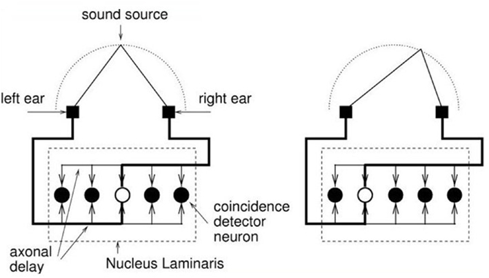
Figure 1. The barn owl auditory system (nucleus laminaris) consists of a decent number of neurons, which all operate as coincidence detectors and which are all connected to axonal delay lines. Depending on the location of the sound source, all the neurons exhibit different activities.

Localization is not only relevant in nature but also in numerous technical applications. The global positioning system (GPS, Misra and Enge, 2006; and in the near future, Galileo, European Commission, 2003, as well) is one of those examples that have penetrated our everyday life. Despite its wide acceptance, GPS has also a few shortcomings. For example, GPS is not available underneath trees nor is it available in indoor environments, such as buildings and tunnels. Furthermore, GPS yields a precision of roughly 8 m, which can be improved to less than 1 m under certain circumstances.

Due to technological advances, many applications, such as Multimodal Smart Appliance Ensembles for Mobile Applications¹, require robust indoor localization systems, that yield a precision in the range of a 1-cm or below at costs as low as possible. Ubisense (Ubisense Ltd.)² and iLoc (Knauth et al., 2009) are very good examples for state-of-the-art indoor localization systems.

A further challenge is induced, if electromagnetic signals are to be used, which is often the case; because electromagnetic signals travel with the speed of light c = 3 × 10⁸ m/s, a resolution of 1 cm corresponds to approximately 30 ps, which cannot be achieved with currently available low-cost digital systems. Because of these requirements, this paper investigates to which extent the main principles of the nucleus laminaris can be realized in digital hardware. To this end, Section II summarizes the localization problem from a technical point of view.

Section III approaches the digital implementation of the neuronal coincidence detectors. Basically, the digital coincidence detector consists of a simple exclusive-or gate, which “mixes” the two incoming signals, and an additional counter, which evaluates the gate’s activation time, which directly corresponds to the signals’ difference, i.e., the phase shift. Because of its internal structure, this localization system is called exclusively XOR-ed counter array, or X-ORCA for short.

X-ORCA’s internal structure is simple and quite regular. These properties make X-ORCA particularly suitable for the implementation on field-programmable gate arrays (FPGAs; Altera Document CII51002-3.1, 2007) and application-specific integrated circuits (ASICs). An FPGA is a digital circuit that consists of thousands of logical gates, which all can be freely configured as well as freely interconnected at the programmers dispense. Section IV briefly discusses a first prototypical implementation on such a digital device.

The first prototype has been tested in various configurations. Section V summaries the experimental results, which indicate that the prototype is able to achieve a resolution as small as 20 ps even though the chosen digital device is clocked as slow as 85 MHz, which corresponds to a duty cycle of about 12 ns.

The initial tests have employed a standard sampling scheme, where the sampling rate f_sample » f_e is much higher than the signal frequency. Section VI explores an additional sampling scheme, known as unfolding-in-time (Hertz et al., 1991). It turns out that this scheme allows for signal frequencies way above the sampling rate; the first prototype easily processes up to 300 MHz as is shown in Section VI, even though the sampling rate is still at 85 MHz. Finally, Section VII concludes this paper with a brief discussion.

2. Problem Description: Localization

Localization is a process that derives new, so-far unknown points from a set of given reference points by evaluating angles and/or distances. Generally, such localization systems come in two flavors: (1) a set of receivers (passive infrastructure) determines the location of an active sender, or (2) a passive receiver derives its own position from the signals emitted by a set of active transmitters. In accordance with the barn owl (and almost all other animals), this paper assumes the first setup.

For educational purpose and for the ease of development, this paper assumes a one-dimensional setup as is illustrated in Figure 2; an extension to a two or three-dimensional setup can be simply realized by duplicating or trippling the one-dimensional setup, and is thus not further discussed in this paper.

FIGURE 2

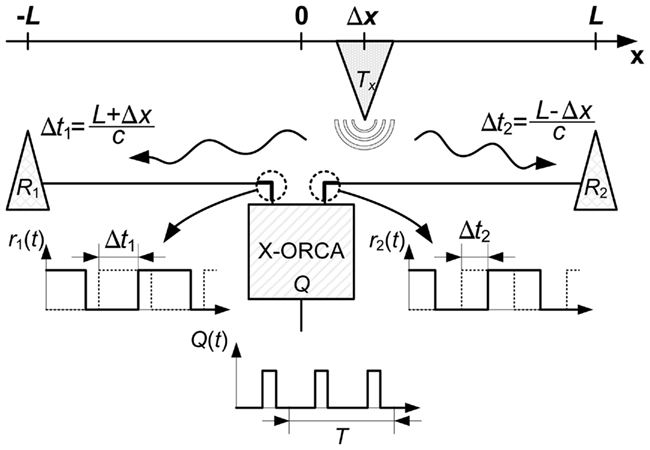
Figure 2. This paper assumes a standard setup, which is simplified to one dimension here. The two receivers read the transmitter’s signals after they have traveled the two distances L + Δx and L − Δx. Thus, the time difference Δt = t₁ − t₂ = 2Δx/c is a result of the transmitter’s off-center position Δx. The system indirectly determines Δt = Δφ/(2πf) by estimating the phase shift Δφ between the two incoming signals r₁(t) and r₂(t).

In a one-dimensional setup, an active transmitter T emits a (sound or electromagnetic) signal s(t) = A sin (2πf(t − t₀)) with frequency f, amplitude A, and time offset t₀. After traveling the two distances L + Δx and L − Δx, the signals arrive at the two receivers R₁ and R₂. Since this traveling happens with a finite speed c, it arrives at the receivers after the time delays Δt₁ = (L + Δx)/c and Δt₂ = (L − Δx)/c.

Normally, both receivers employ an amplifier and a Schmitt trigger, which converts any input signal into a rectangular one. Therefore, the two receivers provide the rectangular signals r₁(t − t₀ − Δt₁) and r₂(t − t₀ − Δt₂), with Δt₁ and Δt₂ denoting the aforementioned time delays that are due to the finite signal traveling speed.

Finally, the localization system has to determine the time difference Δt = Δt₁ − Δt₂ between the two received signals r₁(t − t₀ − Δt₁) and r₂(t − t₀ − Δt₂). If the localization system knows the signal frequency f, it can accomplish this in an indirect way Δt = Δφ/(2πf) by determining the phase shift Δφ between the two signals.

It might be, though, that both the physical setup and the localization system have further internal delays, such as switches, cables of different lengths, repeaters, and further logical gates. However, these internal delays can all be omitted, since they can be easily eliminated in a proper calibration process.

Localization by measuring the time-difference-of-arrival becomes particularly challenging, if the system is based on electromagnetic signals, which travel with the speed of light c ≈ 3 × 10⁸ m/s. For example, an electromagnetic signals travels 1 cm in approximately 33 ps.

3. The X-ORCA Localization System

This section proposes a localization system called X-ORCA, which is an acronym for XOR-ed counter array. On an abstract level, this system has quite the same architecture as the barn owl auditory systems. It consists of two inputs (the two ears), two regular wires (the two axonal delays), and quite a number of coincidence detectors (the neurons).

The description of the (digital) coincidence detectors requires a little more care. First of all, simple logic gates cannot be operating as coincidence detectors. But, “coincidence” of two signals can be interpreted such that there is no difference between them; in other words, they are identical at all times. The difference of two signals is easy to detect, a simple XOR gates can do the job. An XOR gate delivers a logical one, if either of the two inputs has a logical one but not both. Thus, the proportion of a logical one with respect to a logical zero at the output of an XOR gate expresses the phase shift φ between the two inputs (see, also, Section II).

With an XOR gate as the combiner of the two inputs, the task is to measure the average duration of the logical ones at its output. This can be achieved with the circuitry illustrated in Figure 3. The output of the XOR gate is connected to the enable input of a simple counter. This counter increases its value, if at the clock signal (actually the transition from a logical zero to a logical one), the enable input is activated. Thus, the counter value is proportional to the timely proportion of logical ones at the XOR gate’s output and the total number of clock cycles. This value is thus proportional to the phase shift Δφ between both input signals.

FIGURE 3

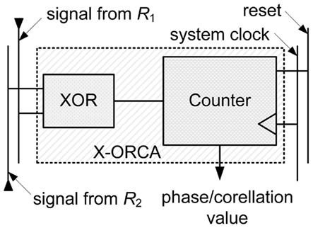
Figure 3. The combination of a simple XOR gate and a subsequent counter is able to operate as a coincidence detector. The counter value is proportional to the proportion of logical ones at the XOR gate’s output and the total number of clock cycles. The counter value is thus proportional to the phase shift Δφ between both input signals.

For example, let us assume an input signal with a frequency of f = 100 MHz and a phase shift of Δφ = π/4 = 45°. Then, if the counter is clocked at a rate of 10 GHz over a signal’s period T = 1/(100 MHz) = 10 ns, the counter will assume a value of v = 25. In this example, all the given numbers, particularly the chosen frequencies, are for educational purposes only, and may not be realistic in a specific implementation.

As has already been seen in the barn owl auditory system, X-ORCA also employs a large number of coincidence detectors (see Figure 4), which are all connected to two reciprocal (anti-parallel) “delay” wires w₁ and w₂ on which the two signals r₁(t) and r₂(t) travel with approximately two third of the speed of light c_w ≈ 2/3c.

FIGURE 4

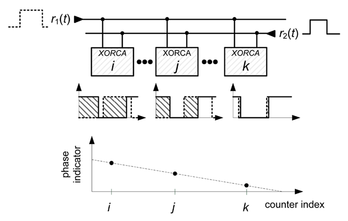
Figure 4. X-ORCA places all phase detectors along two reciprocal (anti-parallel) “delay” wires w₁ and w₂ on which the two signals r₁(t) and r₂(t) travel with approximately two third of the speed of light c_w ≈ 2/3c. Because the two wires w₁ and w₂ are reciprocal, all phase detectors have different internal delays τ_i.

The mode of operation of the X-ORCA system is quite identical to that of the barn owl. Let us start with the coincidence detector (neurons) at which the two inputs match, i.e., both inputs have a vanishing phase shift φ = 0. Then, due to the “delays” along the two wires w₁ and w₂, the coincidence detectors to the right and left observe non-matching inputs, i.e., non-vanishing phase shifts φ ≠ 0. If the delay wires cause a time delay δ between two coincidence detectors, then these detectors observe a total time shift of 2δ. That is, the duration of a logical one is also increased or decrease by 2δ.

Normally, the time difference 2δ is much smaller than the duty cycle of the counter, and would thus not have any effect. However, if sampling over a sufficiently long time span, this tiny time delay will eventually affect the final counter value.

4. The First Prototype

The first X-ORCA prototype was implemented on an Altera Cyclone II FPGA (Altera Document MNLN051805-1.3, 2007). This device charges about 50 USD, offers 33,216 logic elements, and can be clocked at about 85 MHz. The development board, which is required only during research and development, charges about 500 USD and features all the required components, interfaces, and development tools.

Figure 5 shows a top-level view of the X-ORCA prototype. It consists of 140 phase detectors, a common data bus, a Nios II soft core processor (Altera Document NII5V1-7.2, 2007), and a system PLL that runs at 85 MHz. The Nios II processor manages all the counters of the phase detectors, and reports the results via an interface to a PC.

FIGURE 5

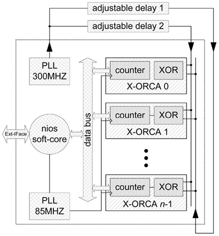
Figure 5. On the top-level, the X-ORCA implementation consists of 140 phase detectors (aligned from top to bottom), a Nios II processor, a first PLL for the system, a second PLL for the localization signal with a frequency of 300 MHz, and just a little bit of additional infrastructure.

Due to the limited laboratory equipment, the transmitter is realized as a simple function generator that emits a sinusoidal signal. In order to focus on the core system, wireless communication capabilities were not employed; rather, the prototype is connected to the function generator via a regular wire as well as a line stretcher (Microlab, 2008). Such a line stretcher can be extended or shorted, and can thus change the signal propagation time accordingly.

It should be noted, though, that X-ORCA’s internal “delay wires” w₁ and w₂ are realized as pure passive internal wires, connecting the device’s logic elements, as previously announced in Section III.

5 Results

Figures 6–11 summarize the experimental results that were achieved with the first X-ORCA prototype under different configurations. Unless otherwise stated, these figures present the counter values v_i of n = 140 different phase detectors, which were clocked at a rate of 85 MHz.

FIGURE 6

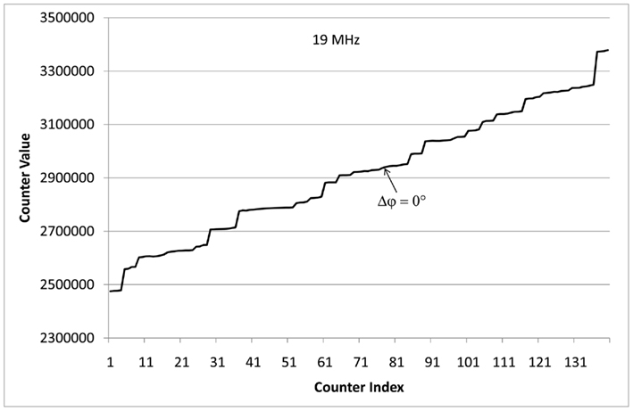
Figure 6. The figure shows the counter values v_i of n = 140 phase detectors when fed with two 19 MHz signals with zero phase shift Δφ = 0.

Figure 6 shows the behavior of the X-ORCA architecture when using the external 19 MHz localization signal. In this experiment, one of the connections from the function generator to the input pad of the development board was established by a line stretcher (Microlab, 2008), whereas the other one was made of a regular copper wire. Figure 6 shows the values v_i of the n = 140 counters, which were still clocked at 85 MHz over a measurement period of 10,000,000 ticks.

In addition, Figure 6 reveals some technological FPGA internals that might be already known to the expert reader: neighboring logic elements do not necessarily have equivalent technical characteristics and are not interconnected by a regular wire grid. As a consequence, the counter values v_i and v_{i + 1} of two neighboring phase detectors do not steadily increase or decrease, which makes the curve look a bit rough. This effect can be compensated. Each counter has a unique and constant internal delay, therefore, the counter values v_i can be plotted over the internal delay τ_i that results in a flat curve as shown in Figure 7.

FIGURE 7

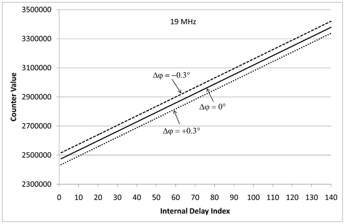
Figure 7. The figure shows the derived counter values v_i of n = 140 phase detectors when fed with two 19 MHz signals with zero phase shift Δφ = 0 (solid line), with about −0.3° phase shift Δφ ≈ −0.3° (dashed line), and with about +0.3° phase shift Δφ ≈ +0.3° (dotted line).

The three graphs in Figure 7 refer to a phase shift of Δφ ∈ {−0.3°, 0, +0.3°}, which corresponds to time delays Δt ∈ −0.02, 0, +0.02 ns. It should be noted that the graph of this figure appears as a straight line, since the internal time delays τ_i span much less than an entire period of the 19 MHz signal.

Figure 8 presents a different view of Figure 7: In the graph, every dot represents the sum v_tot = Σ_iv_i of all n = 140 counter values v_i; that is, an entire graph of Figure 7 is collapsed into one single dot. The graph shows 29 measurements in which the line stretcher was extended by 1 cm step by step. It can be seen that a length difference of Δx = 1 cm decreases v_tot by about 2 million. This result suggests that with a localization of 19 MHz, X-ORCA is able to detect a length difference of about Δx = 1 mm, which equals a time resolution of about 0.003 ns.

FIGURE 8

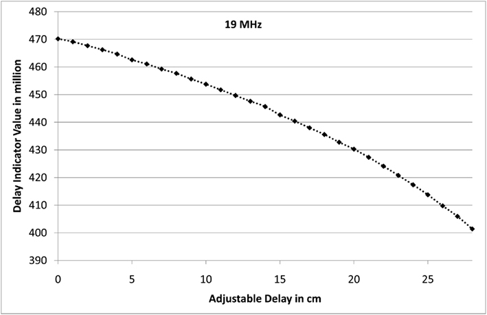
Figure 8. The figure shows the delay value indicator resulting from adjustable delay line lengths when fed with two 19 MHz signals.

The second focus of the practical experiments was to explore the lower limit of the normalized time delay Δt · f. To this end, the prototype was exposed to two localization signals with varying time delays. The localization frequencies were set to f ∈ {1.14 MHz, 111 kHz, 11 kHz}. The results are plotted in Figures 9–11.

FIGURE 9

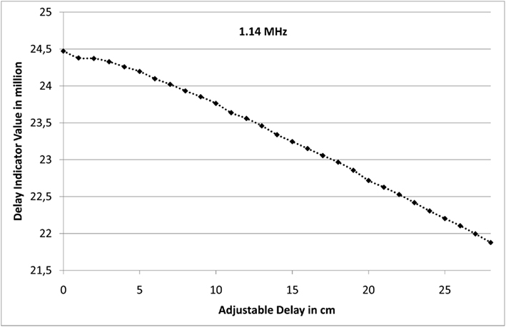
Figure 9. This figure shows the delay value indicator for two 1.14 MHz localization signals for various lengths of the utilized line stretcher.

FIGURE 10

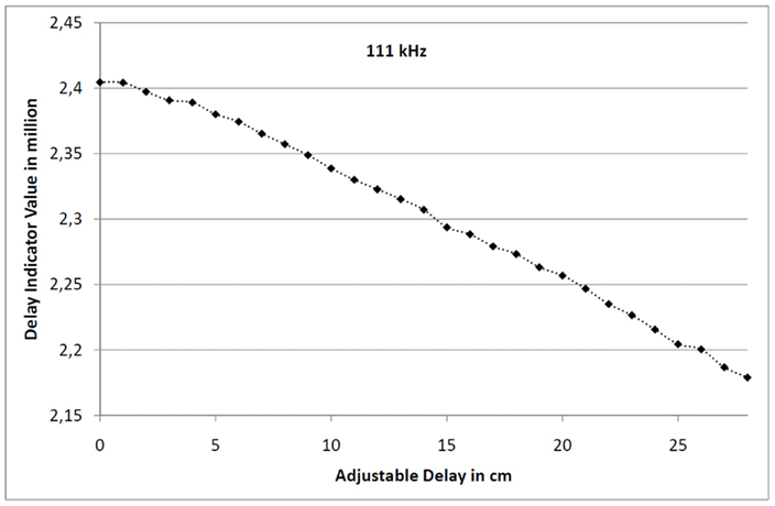
Figure 10. This figure shows the delay value indicator for two 111 kHz localization signals for various lengths of the utilized line stretcher.

FIGURE 11

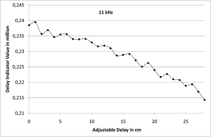
Figure 11. This figure shows the delay value indicator for two 11 kHz localization signals for various lengths of the utilized line stretcher.

All three figures show the very same qualitative behavior. The only difference is the absolute value of the delay value indicator: a decrease of the localization frequency by a factor of 10 leads to a reduction of the delay value indicator by the very same amount; with the identical time delay Δt the phase shift is only a tenth, if the frequency is also just a tenth.

6 Beyond the Limit f_Sample » f_e

From a technical point of view, it might be interesting to explore the upper limit of the frequency f_e of the input signal, which was illustrated as the transmitter T in Figure 2. At first glance, it should be f_e « f_sample way smaller than the sampling frequency f_sample in order to obtain a reasonable resolution of the phase shift Δφ ≥ πf_e/f_sample. That is, the higher the input frequency the more the resolution degrades. However, since both the input and the sample signal are periodic by their very nature, X-ORCA offers other options. One option is known as unfolding-in-time (Hertz et al., 1991), and is described in Subsection VI-A. With this option, the input frequency is not anymore bound to the sampling frequency; rather, it is only limited by the processing speed of the very first stage of the digital implementation device. Subsection VI-B reports results for f_e= 300 MHz, which is simply the limit of the chosen FPGA device.

6.1. Unfolding-in-Time

The upper part of Figure 12 illustrates the “standard” form of sampling a signal Q(t) that has frequency f_e and has thus a signal period T = 1/f_e. Then, the samples could be taken at 0, t, 2t, …, (n − 1)t, with t = T/n denoting the duration between two consecutive samples, and n denoting the number of samples per signal period T. This obviously leads to a resolution of the measurable phase shift Δφ ≥ π/n.

FIGURE 12

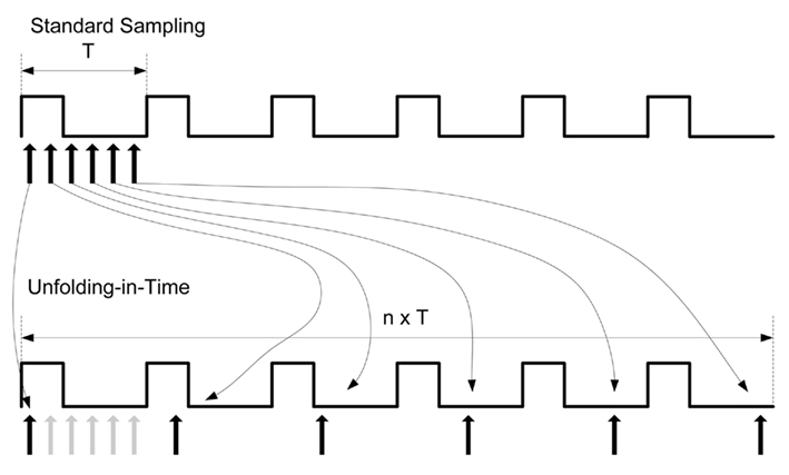
Figure 12. Unfolding-in-time – the sampling points can be distributed over an extended period of time. Rather than sampling at 0, t, 2t, …, (n − 1)t, the samples could also be taken at 0, (t + T), 2(t + T), …, (n − 1)(t + T).

The naive approach discussed above does not take into account that both the input and the sampling signal are periodic by their very nature. In this special case, the sampling points can be distributed over an extended period of time. Rather than sampling at 0, t, 2t, …, (n − 1)t, the samples could also be taken at 0, (t + T), 2(t + T), …, (n − 1)(t + T), as is illustrated in the lower part of Figure 12. As a consequence, the sampling process requires nT time. For the following reason, this process is also known as unfolding-in-time (Hertz et al., 1991): if considering only the modulus t_imodT, all sampling points collapse to the standard sampling procedure 0, t, 2t, …, (n − 1)t as described above. Conversely, by properly choosing a sampling scheme, virtually high sampling frequencies can be obtained, even though the actual sampling frequency f_sample is low.

The chosen time lag “t + T” of the sampling scheme described above can be further relaxed. It suffices to set the time lag to “κt + jT,” with κ and j denoting arbitrary natural numbers, as long as κ and the number of samples n are prime. For example, with n = 4, κ = 3, j = 2, and t = T/4, the samples would be taken at 0, 3t + 2T, 2t + 5T, 1t + 8t, which virtually collapse to 0, t, 2t, 3t.

6.2 Results for f_e = 300 MHz

The available laboratory equipment did not allow for external localization frequencies f_e larger than 19 MHz. Therefore, the second set of experiments utilized a second system-internal PLL (see, also, Figure 5), which runs at 300 MHz.

Figure 13 shows the n = 140 counter values v_i for two 300 MHz (localization) signals that have a zero phase shift Δφ = 0 (solid line), a phase shift Δφ = −30.9° (dotted line), and a phase shift Δφ = +29.5° (dashed line). The input signals were sampled 1,000,000 times, which corresponds to an averaging over 196 periods, with virtually 5100 samples per period of the localization signal (please, see also the discussion presented in Subsection VI-A). It can be clearly seen that the minimum is at counter index no. 32 with increasing counter values to the right and left as can be expected from X-ORCA’s internal architecture.

FIGURE 13

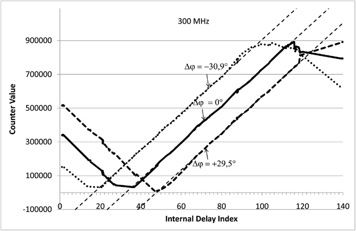
Figure 13. The figure shows the counter values v_i of n = 140 phase detectors when fed with two 300 MHz signals with zero phase shift Δφ = 0 (solid line), with a phase shift Δφ = −30.9° (dotted line), as well as with a phase shift Δφ = +29.5° (dashed line).

Figure 13 shows the same qualitative behavior already shown in Figure 7. That is, already the first prototype is able to determine the phase shift of two 300 MHz signals, even though these signals are sampled at only 85 MHz. The figure also shows that a time difference of Δt ≈ 0.3 ns consistently shifts the “counter curve” by about 15 counters. This results suggests that at 300 MHz, the prototype would be able to detect a time delay as small as Δt = 0.02 ns, which equals to a length resolution of about Δx ≈ 6 mm.

Unfortunately, the available FPGA device does not allow for higher frequencies of the localization signal, and thus does not allow for finding the true limits for f_e.

7. Discussion

This paper has presented a digital implementation, of the barn owl’s nucleus laminaris. The model is called X-ORCA, and is intended to be used in technical applications, such as localization. In its core, X-ORCA exploits the finite traveling speed of signals along anti-parallel wires, and estimates the timing landscape by employing a large number of rather imprecise correlation detectors.

The first prototype runs on a rather old Altera Cyclone II board, and achieves a resolution of about 20 ps for input signals of up to 300 MHz. The obtained resolution in time corresponds to a spatial resolution of about 6 mm, if using electromagnetic signals and having suitable sensors.

Unfortunately, the available laboratory equipment did not allow to test the true limits of the first prototype. This particularly applies to the maximal frequency f_e of the localization signal and to the achievable resolution with respect to Δx. These tests will be certainly subject of future research.

Future research will also be devoted to the integration of wireless communication modules. The best option for that approach seems to be the utilization of a software-defined radio module, such as the Universal Software Radio Peripheral 2 (USRP2; Ettus Research LLC³). Finally, future research will port the first prototype onto more state-of-the-art development boards, such as an Altera Stratix V FPGA (Altera Document SV5V1-1.0, 2010).

Conflict of Interest Statement

The authors declare that the research was conducted in the absence of any commercial or financial relationships that could be construed as a potential conflict of interest.

Acknowledgments

The authors gratefully thank Volker Kühn and Sebastian Vorköper for their helpful discussions. This work was supported in part by the DFG graduate school 1424. Special thanks are due to Matthias Hinkfoth for valuable comments on draft versions of the paper.

Footnotes

1. ^http://www.informatik.uni-rostock.de/musama.html
2. ^http://www.ubisense.net
3. ^http://www.ettus.com

References

Altera Document CII51002-3.1. (2007). Cyclone II Device Handbook. San Jose, CA: Altera Corp.

Altera Document MNLN051805-1.3. (2007). Nios Development Board Cyclone II Edition Reference Manual. San Jose, CA: Altera Corp.

Altera Document NII5V1-7.2. (2007). Nios II Processor Reference Handbook. San Jose, CA: Altera Corp.

Altera Document SV5V1-1.0. (2010). Stratix V Device Handbook. San Jose, CA: Altera Corp.

European Commission. (2003). The Galileo Project – GALILEO Design Consolidation, Guildford.

Hertz, J., Krogh, A., and Palmer, R. G. (1991). Introduction to the Theory of Neural Computation. Redwood City, CA: Addison-Wesley Publishing Co.

Kempter, R., Gerstner, W., and van Hemmen, J. L. (1996). Temporal coding in the sub-millisecond range: model of barn owl auditory pathway. Adv. Neural Inf. Process Syst. 8, 124–130.

Knauth, S., Jost, C., and Klapproth, A. (2009). “iLoc: a localisation system for visitor tracking and guidance,” in Proceedings of the 7th IEEE International Conference on Industrial Informatics 2009 (INDIN 2009), Cardiff, 262–266.

Microlab. (2008). Microlab: “Line Stretchers, SR Series”, Datasheed. Parsippany, NJ: Microlab Company.

Misra, P., and Enge, P. (2006). Global Positioning System: Signals, Measurements, and Performance, 2nd Edn. Lincoln, MA: Ganya-Jamuna Press.