The role of pulvinar in the transmission of information in the visual hierarchy

Visual receptive field (RF) attributes in visual cortex of primates have been explained mainly from cortical connections: visual RFs progress from simple to complex through cortico-cortical pathways from lower to higher levels in the visual hierarchy. This feedforward flow of information is paired with top-down processes through the feedback pathway. Although the hierarchical organization explains the spatial properties of RFs, is unclear how a non-linear transmission of activity through the visual hierarchy can yield smooth contrast response functions in all level of the hierarchy. Depending on the gain, non-linear transfer functions create either a bimodal response to contrast, or no contrast dependence of the response in the highest level of the hierarchy. One possible mechanism to regulate this transmission of visual contrast information from low to high level involves an external component that shortcuts the flow of information through the hierarchy. A candidate for this shortcut is the Pulvinar nucleus of the thalamus. To investigate representation of stimulus contrast a hierarchical model network of ten cortical areas is examined. In each level of the network, the activity from the previous layer is integrated and then non-linearly transmitted to the next level. The arrangement of interactions creates a gradient from simple to complex RFs of increasing size as one moves from lower to higher cortical levels. The visual input is modeled as a Gaussian random input, whose width codes for the contrast. This input is applied to the first area. The output activity ratio among different contrast values is analyzed for the last level to observe sensitivity to a contrast and contrast invariant tuning. For a purely cortical system, the output of the last area can be approximately contrast invariant, but the sensitivity to contrast is poor. To account for an alternative visual processing pathway, non-reciprocal connections from and to a parallel pulvinar like structure of nine areas is coupled to the system. Compared to the pure feedforward model, cortico-pulvino-cortical output presents much more sensitivity to contrast and has a similar level of contrast invariance of the tuning.

1. Introduction

Visual processing in primates is assumed to be hierarchical. The visual activity travels almost sequentially for at least 10 levels of organization (Felleman and Van essen, 1991). This type of cortico-cortical transmission is called feedforward and is generally paired with feedback projections from higher to lower areas (Van Essen et al., 1992). The hierarchical organization is supported by the receptive fields (RF) attributes of neurons, where RFs in higher cortical levels code for progressively more complex properties of the stimuli (Hegdé and Felleman, 2007). Beside this hierarchy in complexity, cortical RFs also increase in size. This increment in both complexity and RFs sizes in higher levels might reflect a gradual feedforward convergence of RFs from early stages (Bullier, 2003).

In parallel to the complexity and growth of the RFs, two basic visual attributes are present in almost all cortical neurons: their firing rate increases smoothly with contrast and the tuning of their responses is contrast invariant. The firing rate of cortical neurons increases sigmoidally with contrast (Albrecht and Hamilton, 1982; Sclar and Freeman, 1982; Sclar et al., 1990). This contrast response function (CRF) of spike activity become progressively steeper as one moves up through the hierarchy (Rolls and Baylis, 1986; Avidan et al., 2002). Cortical cells also seem to maintain a constant tuning to visual stimuli as contrast is varied. In V1 cells, contrast invariance of the tuning to oriented bars is seen across the six cortical layers (Olsen et al., 2012). MT and V4 cells also have this attribute. In higher levels, neurons also seem to show contrast invariant tuning. However, here the detection of tuning curves is less accurate, so the evidence for this has to be confirmed (Baylis et al., 1985).

The propagation of the response to visual stimuli through the cortical hierarchy has so far only received very limited attention in theoretical studies. A simple model to test firing rate transmission is a feedforward model (FF). This model consists in a layered chain of neural population in which a population of a given layer receives inputs from the previous layer. The first layer receives the visual stimulus. Given the non-linear input-output relation of the neuronal populations, chains of such populations will rapidly develop the tendency to a step response, or go to a constant response when the contrast is varied (Cortes, 2008). Such a bimodal response developed in simple FFN is also seen in more realistic layered networks with spiking neurons (Litvak et al., 2003).

In fact, a simple model with connections only between adjacent layers in the hierarchy, both feedforward and feedback, result in a step-function response or constant output for higher layers (Cortes, 2008). To get reasonable CRFs for cortical areas higher in the hierarchy, a shortcut is needed to link hierarchically distant levels. We propose that this shortcut is provided by the Pulvinar nucleus (Pul) of the thalamus. Our assumption is based on: (i) non-reciprocal connections between Pul and visual cortex (Sherman, 2007), (ii) a cortical gradient inside Pul (Shipp, 2003), (iii) Pul microcircuitry with long range connections (Imura and Rockland, 2006). It has been shown (Cortes, 2008) that adding a shortcut through Pul to a simple chain of cortical areas can lead to smooth sigmoidally shaped CRFs for areas high in the hierarchy, provided that the inputs from Pul to the different cortical areas is sufficiently small. However, in that study the increase of size and complexity of the RFs with the layer in the cortical hierarchy was not taken into account. Presumably the increase of RF complexity is, at least partially, due to the specificity of the cortico-cortical feedforward connections. On the other hand, the Pul, which is a much simpler structure than visual cortex, is unlikely to have cells with RFs of comparable complexity as higher layers in the visual cortex. This raises the question whether the input from Pul to cortex, necessary to obtain smooth sigmoidal tuning curves in the higher cortical areas, does not disrupt the formation of complex RFs in these areas. To study this issue, we create a firing rate model in which the connectivity of the cortico-cortical feedforward pathway increases both the complexity and size of the RFs as one move higher in the hierarchy. We investigate networks with purely cortico-cortical connections (feedforward and feedforward-feedback), and networks with also cortico-pulvino-cortical connections (feedforward-Pul and feedforward-feedback-Pul). For these networks we analyze both the CRF and contrast invariance of the response tuning in different levels of the hierarchy, to establish that cortico-pulvino-cortical connections can significantly improve both the smoothness of the CRF and contrast invariance in higher cortical areas.

2. Materials and Methods

We study a network of interconnected cortical areas that mimics some of the properties of the visual cortex. The system is hierarchical with L layers, with, as one ascends the hierarchy, RFs of increasing size and complexity. This behavior of the RFs through the hierarchy is observed in the two processing streams of the visual cortex: the dorsal and ventral stream. At the same time, taking into account the remarkable homogeneity of the architecture of different visual cortical areas, the units in the network are identical. The increase in size and complexity are, in our model, due to the pattern of the feedforward connectivity.

For simplicity we consider a network with a one-dimensional “visual” input. The network has L areas which each cortical area consists of 2^L units. In the first layer of the hierarchy, our model of V1, the response of these units describes the average response of a group of neurons with the receptive fields at the same position. The feedforward inputs into units of higher cortical areas are combinations of the output of 2 adjacent units in the area below it in the hierarchy. Thus, each time one goes up one level in the hierarchy, the number of receptive field positions decreases by a factor of two. At the same time, at each position, there are different units which receive different combinations of inputs from the two units in the lower areas as described below. Because of this, as one ascends the hierarchy the number of “types” of receptive fields is doubled with in each layer.

Next we add feedback connections from units in higher cortical areas to the area just below it, with feedback connections only to those units from which the higher area unit receives input.

Finally we consider the effect of the a pulvinar like structure on the activity of the cortical hierarchy. Our pulvinar model is similar to the model of the cortex, in that it has a hierarchy of layers with receptive fields that increase in size and complexity as one goes up the hierarchy. The major differences between pulvinar and visual cortex is that the number of types of receptive fields does not double as one ascends the hierarchy and that in the pulvinar units in layer ℓ receives feedforward inputs from layers 1 to ℓ − 1, not just from layer ℓ − 1, as is the case in our cortex model.

2.1. The Model of the Units

Each unit in the model consists of two subunits, with “On” and “Off” cells respectively. The subunits consists of interconnected excitatory and inhibitory populations. For simplicity we assume that these can be described by one effective population, whose effective input is the difference between the input into the excitatory neurons and the inhibitory ones. If the effective input into the “On” and “Off” subunits is I₊ and I₋ respectively, their rates, r₊ and r₋, satisfy

${\tau }_r\frac{d}{dt}{r}_{\pm }=-r_{\pm }+F\left(I_{\pm }\right),$(1)

where τ_r is the time constant and f is a sigmoidal functions, satisfying F(I) = [1 + exp(−I + Ith)]⁻¹. Here, Ith is the threshold.

As a further simplification we assume that I₋ = −I₊ = I and the rates of the “On” and “Off” groups can be combined into an effective rate, r = r₊ − r₋ with an effective transfer function, f, given by

$f\left(I\right)=\frac{1}{1+exp\left(-I+I\text{th}\right)}-\frac{1}{1+exp\left(I+I\text{th}\right)}.$(2)

The threshold Ith is the same for all cortical units.

Pulvinar units are modeled the same way with the effective rate s of the pulvinar unit having the same time constant, τ_r, and the effective transfer function also satisfying equation (2), all be it that Ith can be different for pulvinar units. In the full model we will use $I_{th}^{ctx}$ and $I_{th}^{pul}$ to denote threshold for the cortical and pulvinar units respectively. When we consider a model consisting only of the cortical hierarchy we will the denote the threshold by Ith for simplicity.

The transfer function, f, can be written as

$f\left(I\right)=\frac{\text{sinh}\left(I\right)}{\text{cosh}\left(I\right)+\text{cosh}\left(I\text{th}\right)}.$(3)

Note that the transfer function does not change if we replace Ith by −Ith, so that without loss of generality we can assume that Ith ≥ 0. The first and second derivatives of f are given by

$\begin{array}{llll}{f}^{\prime }\left(I\right)& =\frac{1+\text{cosh}\left(I\right)\text{cosh}\left(I\text{th}\right)}{{\left[\text{cosh}\left(I\right)+\text{cosh}\left(I\text{th}\right)\right]}^2}\text{and}& & \\ f^{\prime \prime }\left(I\right)& =\frac{\text{sinh}\left(I\right)\left[{\text{cosh}}^2\left(I\text{th}\right)-\text{cosh}\left(I\right)\text{cosh}\left(I\text{th}\right)-2\right]}{{\left[\text{cosh}\left(I\right)+\text{cosh}\left(I\text{th}\right)\right]}^3},& & \text{(4)}\end{array}$

respectively.

The transfer function increases monotonically from −1 to 1 as I goes from minus to plus infinity and has 1 or 3 inflection points. The inflection points are found by solving f ′′(I) = 0 and are given by sinh(I) = 0 and cosh(I) = [cosh² (Ith) − 2]/cosh(Ith). The first of these always has a solution I = 0. There are two other inflection points at $I=\pm \text{In}\left(z+\sqrt{z^2-1}\right),$ where z = [cosh²(Ith) − 2]/cosh(Ith) if cosh(Ith) > 2, or $I\text{th}>ln\left(2+\sqrt{3}\right)\approx 1.317.$

Figure 1 shows how the transfer function transforms the input into the output rate. The Figure plots the output rate, r_out = f (W_FFr_in) as a function of the input rate, r_in, for different values of the threshold, Ith, and different values of the synaptic strength, W_FF.

FIGURE 1

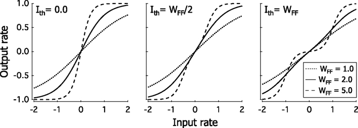
Figure 1. Examples of input-output transfer functions at different values of the threshold, Ith. In each plot, the strength W_FF is also changed to analyze changes in linearity of curves. In all three conditions, low values of W_FF produces a reasonably linear response. As W_FF increases the response curves increase in non-linearity. For Ith = 0.0, when W_FF is large, the curve is steep, and the only one inflection point occurs at r₀ = 0. Three inflection points are seen when the threshold is sufficiently large $\left(\text{cosh}\left(I\text{th}\right)>\sqrt{2}\right).$ The shape of the input-output curves is a combination of two sigmoidal functions in which the non-linearity increase in as W_FF becomes larger. The inflection points are at r₀ = 0 and at $r_0=\pm \text{In}\left(z+\sqrt{z^2-1}\right)/W_{FF},$ where $z=\left({\text{cosh}}^{2}I\text{th}-2\right)∕\text{cosh}I\text{th}.$

2.2. Network Architecture

For the cortical architecture we consider neuroanatomical properties of the ventral visual stream. In the cortex, the ventral stream starts in V1, cross early visual areas until arrives to V4, and ends in the inferotemporal (IT) cortex (Van Essen et al., 1992). Classically, the ventral stream is related with object identification. Despite the fact that feedforward connections between ventral stream cortical areas traverse several hierarchical levels, most of the connections cross only 1 or 2 levels. This number of levels traversed is also seen in feedback connections (Felleman and Van essen, 1991). On the other hand, in monkeys the ventral stream receives connections directly from the Pul (Kaas and Lyon, 2007). These pulvinar connections have been postulated to follow a gradient of connectivity, from low to high hierarchical levels (Shipp, 2003). Also, the cortico-pulvino-cortical pathway is described to have to different loop of connections while here we consider the open type (see Pulvinar Architecture; Sherman, 2007).

By assuming the previously described requirements, in our model the input into a cortical units in area ℓ has three components: cortical feedforward input from area ℓ − 1, cortical feedback from ℓ + 1 and pulvinar input from pulvinar area ℓ − 1. The exception to these inputs projections are first and last cortical areas. The first cortical area receives only feedforward input from LGN and feedback from cortical area 2, but lacks inputs from the pulvinar. The last cortical layer, layer L, does not receive cortical feedback input.

2.2.1. Intracortical connections

We account for the increasing size and complexity of the receptive fields as one moves up the cortical hierarchy by assuming that in area ℓ the units receive input from two neighboring units in area ℓ − 1. For example, units at position 1 in area 1 receive inputs from the units at position 1 and 2 of the input, so layer 0, while units at position 2 receive feedforward inputs from area 0 units at position 3 and 4, etc. At each position in layer 1 two units with different receptive field types. In the first the input is proportional to the sum of the outputs of the two units in layer 0 which project to it, in the other the input is proportional to their difference. In layer 2 units at position i receive inputs from units at position 2i −1 and 2i in layer 1, and there are 4 kinds of receptive fields. The input into units with type 1 receptive fields take as argument the sum of output of the two units with type 1 receptive fields in layer 1. For type 2 units the argument is the difference between these. Type 3 receptive fields have as input the sum of the outputs of the type 2 units in layer 1, while type 4 units have the difference of these two as input. This algorithm is repeated for higher layers. This results in a system in which for layer ℓ there 2^{L − ℓ} positions, at each of which there are 2^ℓ different types of receptive fields (Figure 2).

FIGURE 2

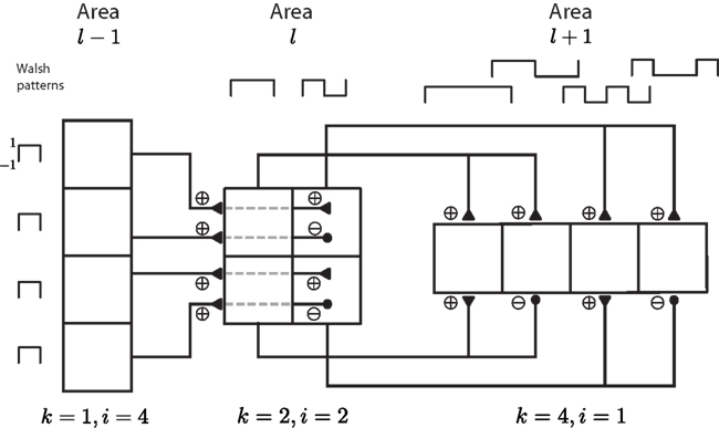
Figure 2. Schematic representation of the feedforward connections. The sign of the connections represent Walsh pattern sequences from area ℓ − 1 to area ℓ + 1. The combination of inputs from pairs of units creates the receptive fields in the next layer. The four units, i, in area ℓ − 1, have the same type of receptive field (k = 1) at different positions. The summation and subtraction of the output of two units produces two different types of RFs in area ℓ, the size of these RFs is twice as large, and the number of RF positions is reduced by a factor of two. This process is repeated for the connections from area ℓ to area ℓ + 1. Thus in layer 0 we have only 1 type of RF at 2^L positions, in layer 1 we have 2 types of RFs, with 2^{L − 1} positions, with each unit responsive to 2 neighboring positions in layer 0, while in layer L we have 2^L types of RFs at 1 position, with each unit responsive to the whole input range.

We denote the rate of the unit of layer ℓ at position i with receptive field type k with $r_{k,i}^{\ell }$ and its feedforward input by $I_{k,i}^{\ell }\left(FF\right)$ for 1 ≤ ℓ ≤ L − 1 the feedforward input is given by

$\begin{array}{llll}{I}_{2k-1,i}^{\ell }\left(FF\right)& =W_{FF}\left(r_{k,2i-1}^{\ell -1}+r_{k,2i}^{\ell -1}\right)& & \\ I_{2k,i}^{\ell }\left(FF\right)& =W_{FF}\left(r_{k,2i-1}^{\ell -1}-r_{k,2i}^{\ell -1}\right),& & \text{(5)}\end{array}$

for i = 1, …, 2^{L − ℓ} and k = 1, …, 2^ℓ. Here W_FF is the strength of the feedforward connections.

For ℓ = 1 two types of receptive field exists, k = 1, 2 and the feedforward input is, for i = 1, …, 2^{L − 1}, given by $I_{1,i}^1\left(FF\right)=W_{FF}\left(r_{2i-1}^0+r_{2i}^0\right)$ and $I_{2,i}^1\left(FF\right)=W_{FF}\left(r_{2i-1}^0-r_{2i}^0\right),$ where $r_i^0$ is the output of the Ith LGN unit.

Units in area ℓ receive reciprocal input from those units in area ℓ + 1 onto which they project. This feedback input has the same sign as the feedforward input but is modulated by connection strength W_FB. The cortical feedback input, $I_{k,i}^{\ell }\left(FB\right),$ in the unit with receptive field type k at position i in layer ℓ, is given by:

$\begin{array}{llll}{I}_{k,2i-1}^{\ell }\left(FB\right)& =W_{FB}\left(r_{2k-1,i}^{\ell +1}+r_{2k,i}^{\ell +1}\right)& & \\ I_{k,2i}^{\ell }\left(FB\right)& =W_{FB}\left(r_{2k-1,i}^{\ell +1}-r_{2k,i}^{\ell +1}\right),& & \text{(6)}\end{array}$

Units in the L_th cortical area have no feedback inputs. To compensate for this we assume that the strength of the feedforward connection to the last area is W_FF + W_FB rather than W_FF. Note also that in the layer L the receptive fields span the whole input range and there is only 1 position (i = 1). The feedforward input into layer L units is given by

$\begin{array}{llll}{I}_{2k-1,1}^L\left(FF\right)& =\left[W_{FF}+W_{FB}\right]\left(r_{k,1}^{L-1}+r_{k,2}^{L-1}\right)& & \\ I_{2k,1}^L\left(FF\right)& =\left[W_{FF}+W_{FB}\right]\left(r_{k,1}^{L-1}-r_{k,2}^{L-1}\right).& & \text{(7)}\end{array}$

It is well known that the synaptic connections from one cortical area to another emanate from pyramidal neurons (Rodney et al., 2004). So, both feedforward and the feedback pathways are are excitatory. However, in the model here we are considering effective inputs. The effective connection are positive if the excitatory population in the presynaptic “On” unit project to the excitatory “On” population and the inhibitory “Off” population of the postsynaptic unit while the presynaptic excitatory “Off” population projects to the excitatory “Off” and inhibitory “On” populations in the postsynaptic unit. The effective connection is negative if the presynaptic “On” cells project to the inhibitory “On” and excitatory “Off” cells in the postsynaptic unit and similar for the excitatory presynaptic “Off” cells.

2.2.2. Pulvinar architecture

The Pul is the largest thalamic nucleus in primates and it presents anatomical and physiological properties that involve with visual cortical transmission. The Pul has two topographic maps that traverse retinotopically the lateral (PL) and inferior (PI) subdivisions of the Pul. These two subdivisions connect directly with the ventral stream of the cortex. The other two subdivision of the Pul, medial (PM) and anterior divisions (PA), connect partially to cortical areas of the dorsal stream (Stepniewska, 2003; Kaas and Lyon, 2007). RFs of pulvinar neurons has simple visual features that correspond with the cortical areas that they target. RFs of cat and monkey pulvinar neurons have small and large diameter sizes, are driven by orientated bars with a broad tuning responses as well as motion to textured patterns, and color-sensitive attributes (Casanova, 2003).

The major source of visual inputs to Pul come from the visual cortex. Lesions in striate cortex of macaque eliminated the visual response of pulvinar neuron. This input from the cortex is represented as a gradient inside the Pul. Shipp (2003), based on cortico-thalamic and thalamo-cortical connections, postulates the existence of a “cortical gradient” in the Pul. While injections with dual tracer in V1 and V4 label preferentially respective medio-caudal and latero-rostral pulvinar areas, injection in V2 target lateral within Pul, and inferior temporal cortical areas, medial within Pul. On the other hand, injections in area V1, that represent retinotopic position of either the upper and lower contralateral hemivisual field, label neurons in respective hemifield of both PL and PI. Thus, a fronto-occipital axis in the cortex is reproduced as a medio-lateral gradient in the pulvinar (medio-lateral cortical axis rotates to a rostro-caudal gradient in the thalamus). In addition to the gradient observed in the Pul, the cortico-pulvino-cortical loop has two types of connections. In one subgroup the cortical layer VI project to a pulvinar region, which in turn send back to same cortical area but to layer IV (“Reciprocal connections,” similar to connections between V1 and the LGN). In the other, connections arise from cortical layer V and end in a non-reciprocal pulvinar region. In turn, this pulvinar region sends back orthogonally to the cortex. These latter are known as “non-reciprocal connections” and it is considered here as an open loop (Sherman, 2007).

In addition to projections from and to the cortex, the Pul also has a local circuitry. Recently works show at least four intrinsic interactions: (i) axons type I are branched and highly divergent (1.0–3.0 mm), to the extent that they can easily be shown to cross over subdivisions (Rockland, 1996, 1998); (ii) Long range inhibitory interneurons traverse areas in 1.0 mm of length (Imura and Rockland, 2006); (iii) The existence of “bridges” between PI subdivisions that stain to calcium binding protein calbindin and to substance P (Stepniewska, 2003); (iv) Inhibitory inputs from the reticular nucleus which receives excitatory branches from the cortico-thalamic and thalamo-cortical axons (Sherman and Guillery, 2000).

For the Pul architecture the previous attributes are considered. The Pul is modeled similarly to the cortex. However, each pulvinar area has at most 4 types of RFs, the patterns corresponding to k = 1, 2, 2^{ℓ − 1}, 2^ℓ, for l ≥ 2. Reciprocal cortico-pulvino-cortical interactions mainly have the effect of changing the effective if modifying the effective cortical transfer functions, so that, in the interest of simplicity only the non-reciprocal cortico-pulvino-cortical pathway is assumed and the gradient inside the Pul is modeled as a feedforward pathway with long range connections. Pulvinar units in area ℓ receive input from cortical units in area ℓ and from pulvinar units in areas 1 to ℓ – 1. The input $J_{k,i}^{\ell }\left(PC\right)$ from cortex to unit i of type k in pulvinar region ℓ is given by

$\begin{array}{llll}{J}_{2k-1,i}^{\ell }\left(PC\right)& =W_{PC}\left(r_{k,2i-1}^{\ell }+r_{k,2i}^{\ell }\right)& & \\ J_{2k,i}^{\ell }\left(PC\right)& =W_{PC}\left(r_{k,2i-1}^{\ell }-r_{k,2i}^{\ell }\right),& & \text{(8)}\end{array}$

for l = 3, …, L − 1, i = 1, …, 2^{L − ℓ − 1} and k = 1, 2^{ℓ − 1}.

The long range interactions in the pulvinar are mediated through large GABAergic interneurons (Imura and Rockland, 2006). Thus the connections between units in different pulvinar layers are through inhibitory synapses. Nevertheless, as for cortico-cortical interactions, the effective coupling can be positive or negative, depending on whether the postsynaptic target neurons are excitatory or inhibitory. The input $J_{k,i}^{\ell }\left(PP\right)$ from the rest of the pulvinar satisfies:

$\begin{array}{l}{J}_{2k-1,i}^{\ell }\left(PP\right)=\frac{1}{1+W_{LP}}(W_{FP}\left[s_{k,2i-1}^{\ell -1}+s_{k,2i}^{\ell -1}\right]\\ +\frac{W_{LP}}{2}\left[J_{k,2i-1}^{\ell -1}\left(PP\right)+J_{k,2i}^{\ell -1}\left(PP\right)\right])\\ J_{2k,i}^{\ell }\left(PP\right)=\frac{1}{1+W_{LP}}(W_{FP}\left[s_{k,2i-1}^{\ell -1}-s_{k,2i}^{\ell -1}\right]\\ +\frac{W_{LP}}{2}\left[J_{k,2i-1}^{\ell -1}\left(PP\right)+J_{k,2i}^{\ell -1}\left(PP\right)\right]),\end{array}$(9)

Here we have used $s_{k,i}^{\ell }$ denote the rate of the pulvinar units. The units in pulvinar layer 1 do not receive input from the rest of the pulvinar, $J_{k,i}^1\left(PP\right)=0$, while for pulvinar layer 2 we assume that J(PP) is given by

$\begin{array}{llll}{J}_{2k-1,i}^2\left(PP\right)& =W_{FP}\left[s_{k,2i-1}^1+s_{k,2i}^1\right]& & \\ J_{2k,i}^2\left(PP\right)& =W_{FP}\left[s_{k,2i-1}^1-s_{k,2i}^1\right].& & \text{(10)}\end{array}$

This specifies how the pulvinar input to pulvinar units depends on the activity in the previous areas. For example in pulvinar layer 4, the input $J_{k,i}^4\left(PP\right)$ for k = 1 is given by the combination of the pulvinar-feedforward and the long range connections

$\begin{array}{l}{J}_{1,i}^4=\frac{W_{FP}}{1+W_{LP}}\left[s_{1,2i-1}^3+s_{1,2i}^3\right]\\ +\frac{W_{LP}}{2\left(1+W_{LP}\right)}\left[J_{1,2i-1}^3\left(PP\right)+J_{1,2i}^3\left(PP\right)\right]\\ =\frac{W_{FP}}{1+W_{LP}}(\left[s_{1,2i-1}^3+s_{1,2i}^3\right]\\ +\frac{W_{LP}}{2\left(1+W_{LP}\right)}\left[s_{1,4i-3}^2+s_{1,4i-2}^2+s_{1,4i-1}^2+s_{1,4i}^2\right])\\ +{\left(\frac{W_{LP}}{2\left(1+W_{LP}\right)}\right)}^2[J_{1,4i-3}^2\left(PP\right)\\ +J_{1,4i-2}^2\left(PP\right)+J_{1,4i-1}^2\left(PP\right)+J_{1,4i}^2\left(PP\right)]\\ =\frac{W_{FP}}{1+W_{LP}}(\left[s_{1,2i-1}^3+s_{1,2i}^3\right]\\ +\frac{W_{LP}}{2\left(1+W_{LP}\right)}\left[s_{1,4i-3}^2+s_{1,4i-2}^2+s_{1,4i-1}^2+s_{1,4i}^2\right]\\ +{\left(\frac{W_{LP}}{2\left(1+W_{LP}\right)}\right)}^2[s_{1,8i-7}^1+s_{1,8i-6}^1+s_{1,8i-5}^1\\ +s_{1,8i-4}^1+s_{1,8i-3}^1+s_{1,8i-2}^1+s_{1,8i-1}^1+s_{1,8i}^1]).\end{array}$(11)

A direct expression of $J_{k,i}^{\ell }$ in the activity of units in the previous layers for different values of k and ℓ is straightforward.

Finally, the input from pulvinar to cortex, I(CP), is given by:

$\begin{array}{llll}{I}_{2k-1,i}^{\ell }\left(CP\right)& =W_{CP}\left[s_{k,2i-1}^{\ell -1}+s_{k,2i}^{\ell -1}\right]& & \\ I_{2k,i}^{\ell }\left(CP\right)& =W_{CP}\left[s_{k,2i-1}^{\ell -1}-s_{k,2i}^{\ell -1}\right],& & \text{(12)}\end{array}$

where $s_{k,i}^{\ell }$ is the output of pulvinar unit for k = 1, 2, 2^{ℓ − 1}, 2^ℓ, and $s_{k,i}^{\ell }=0$ otherwise.

2.3. LGN Input

The spatial filtering properties of LGN neurons is such that for natural visual stimuli the response of different LGN neurons is uncorrelated (Simoncelli and Olshausen, 2001). In accordance with this we assume that for visual stimuli the effective output, $r_i^0,$ of the LGN units at position i can be written as

$r_i^0=\sigma x_i,$(13)

where the variables x_i are independently drawn from Gaussian distribution. Note that as for the cortical and pulvinar units the effective rate is the difference between the response of the “On” and “Off” cells and hence can be either positive or negative.

The prefactor σ in equation (13) is an increasing function of the contrast and scales the whole LGN response where σ = 1 represents an input with contrast 100%. A basic assumption in study is that, if the same visual scene is presented at different contrasts, the effect the contrast cage on the LGN output is to modulate the output of all LGN units by the same factor. Thus increasing the contrast amounts to increasing σ, while keeping the random variables x_i the same. On the other hand if one considers different visual scenes with the same contrast, σ should be kept the same, while different random variables x_i should be drawn for each scene.

2.4. Optimization Criteria

We analyze networks in two conditions, and so, we work out two different optimization procedures. We first explore the behavior of networks when a homogeneous input, $r_i^0=r_0,$ is applied to the first layer. This give some insight of the properties of the model. Secondly, we assume a visual stimuli where properties have been described in the previous section.

2.4.1. Homogeneous input

The activity of the last cortical area is the summary of the previous ones. When a discontinuous or very small change of its response occurs for an increase in contrast of the input, the output is not very useful to estimate the stimulus. The optimal output of layer L is one that spans the whole range of outputs and varies more or less linearly with the input, r₀. However, these two requirements are in conflict. For example, when a homogeneous input from −1, 1 is applied to the feedforward model, a large W_FF assures utilization of the whole dynamic range between −1 and 1, but yields an extremely non-linear curve. Instead, for small W_FF the curve that plots r_L against r₀ appears much more linear, but only covers a small part of the output range. An optimization criterion that penalizes both these extreme cases and measures how good the network is able to transmit information about stimulus contrast is the entropy of the output distribution if the r₀ is distributed homogeneously between −1 and 1. The entropy is low both in the case where the input-output relation is close to a step-function and also when the output range is small. Thus, to optimize the output of the unit $r_{1,1}^L$ of different networks when a homogeneous input is applied in layer 1, we determine parameters for which the entropy, H, given by

$H=-{\int }_{-1}^{1}dr{P}_L\left(r\right)log{P}_L\left(r\right)$(14)

is maximal. Here, P_L(r) is the probability density distribution of the Lth layer.

We now derive an expression for H, where the relation r_L = F(r₀) is known and r₀ is drawn from a homogeneous distribution between −1 and 1. For a small Δr this probability will be

$P_L\left(r\right)\Delta r=\text{Prob}\left(r<r_L<r+\Delta r\right).$(15)

Since r_L = F(r₀), this is equal to

$\begin{array}{l}{P}_L\left(r\right)\Delta r=\mathrm{Pr}\text{ob}\left(F^{-1}\left(r\right)<r_0<F^{-1}\left(r+\Delta r\right)\right)\\ \approx \mathrm{Pr}\text{ob}\left(F^{-1}\left(r\right)<r_0<F^{-1}\left(r\right)+{F^{\prime }}^{-1}\left(r\right)\Delta r\right).\end{array}$(16)

Here F ′⁻¹ is the derivative of F^–1, the inverse of F.

Since r₀ is drawn from a uniform distribution between −1 and 1, Prob (F⁻¹(r) < r₀ < F⁻¹ (r) + F ′⁻¹(r) Δr) is equal to F ′⁻¹(r)Δr/2. Together with F ′⁻¹(r_L) = 1/F ′(r₀) this yields

$P_L\left(r_L\right)=\frac{1}{2F^{\prime }\left(r_0\right)}.$(17)

Inserting this into equation (14), the entropy is given by

$H=\frac{1}{2}{\int }_{-1}^{1}d{r}_{0}log2F^{\prime }\left(r_0\right),$(18)

where we have used dr_L = F ′(r₀)dr₀.

2.4.2. Natural visual stimuli

That was the optimization procedure for networks in which a homogeneous input is used, $r_i^0=r_0.$ We use similar optimization principle for the analysis of the visual input. In this case, a random input is applied in $r_i^0=\sigma x_i,$ where σ codes for contrast and x_i is independently drawn from a Gaussian with zero mean and unit variance. Here, changes in contrast are changes in σ without changing x_i. To ensure that the response is sensitive to contrast and the tuning is maximally contrast invariant, we want that the amplitude of the 2^L dimensional vector $\overrightarrow{V}$ given by $V_k=r_{k,1}^L$ varies smoothly with σ², while its direction changes as little as possible as σ is varied.

We define the output amplitude, F, as the average length of the output for LGN inputs with contrast σ, $F\left(\sigma \right)=⟨\left|\overrightarrow{V}\right|⟩,$ where the average is over the variables x_i. Similar to the analysis of the homogeneous input condition, we aim for an amplitude function F that is as linear as possible and uses the dynamic range maximally. This we ensure by imposing a cost function, H_L, defined as $H_L={\int }_0^{1}d\sigma log\left(F^{\prime }\left(\sigma \right)\right),$ for this property. If H_L = L log2, the output scales linearly and exploits the whole dynamic ranges. It decreases if less of the dynamic range is used or the response scales non-linearly.

To explore whether the network can maintain contrast invariant tuning, we calculate the mean of separation distance S between normalizes output vectors $\overrightarrow{e}\left(\sigma \right)=\overrightarrow{V}\left(\sigma \right)∕\left|\overrightarrow{V}\left(\sigma \right)\right|$ and $\overrightarrow{e}\left({\sigma }^{\prime }\right)=\overrightarrow{V}\left({\sigma }^{\prime }\right)∕\left|\overrightarrow{V}\left({\sigma }^{\prime }\right)\right|$ for LGN inputs $r_i^0=\sigma x_k$ and $r_i^0={\sigma }^{\prime }{x}_k$ respectively, $S={\int }_0^{1}d\sigma {\int }_0^{1}d{\sigma }^{\prime }\overrightarrow{e}\left(\sigma \right)\cdot \overrightarrow{e}\left({\sigma }^{\prime }\right).$ If S = 1, the vectors are in the same direction for all contrasts. As the direction changes more with contrast, S decreases.

For the optimization of the network parameters define a total error $E=-2S-e^{H_L}$ that takes both these factors into account. In both optimization criteria, the homogeneous and the visual input, we attempt to minimize the error of the functions. Thus, we want to maximize both S and H_L. So, given the parameter space of models we use the Powell’s method (Press et al., 1992).

3. Results

In our model we assume that natural stimuli are characterized by inputs $r_i^0$ which are given by $r_i^0=\sigma x_i,$ where the variables x_i are independently drawn from from a Gaussian with mean 0 and variance 1. However, to get some insight into the properties of the model, we first analyze its response to a simpler input, $r_i^0=r_0.$

3.1. Response to Homogeneous Input

3.1.1. Purely feedforward transmission

In the purely feedforward model (W_FB = W_CP = W_PC = 0), the activity is propagated sequentially through the cortical areas until reach l = L. The input is varied in magnitude to mimic changes in contrast of the stimulus.

If $r_i^0$ is the same for all units, $r_{1,j}^1$ will also be identical for all j. As a result, $r_{1,i}^2$ will also be independent of i, etc. At the same time, because $r_i^0$ is the same for all i, $r_{2,j}^1$ will be zero for all j. Extending this logic to larger ℓ, we see that $r_{k,i}^{\ell }=0$ for K = 2, 3, …, 2^{ℓ − 1}, while $r_{1,i}^{\ell }=r_{\ell }$ is the same for all i. The equilibrium rates are given by r₁ = f(W_FFr₀), and

$r_{\ell }=f\left(2W_{FF}{r}_{\ell -1}\right).$(19)

for l ≥ 1.

Figure 3 shows the equilibrium rate as a plotted against r₀ for layers l = 1, 5, and 10, for different values of the feedforward strength and threshold. When W_FF is small the rate in r₁ increases smoothly from approximately −1 to approximately 1 as the input r₀ varies from −2 to 2. For larger ℓ the response is progressively smaller, until for l = 10 the response almost stays at 0. On the other hand, for large W_FF with Ith = 0, r₀ shows a clear sigmoidal response. For larger ℓ the steepness of the sigmoid increases so that for l = 10 the response in almost a step-function. For Ith ≠ 0, the response evolves to a sum of two sigmoids, with thresholds at −Ith/W_FF and Ith/W_FF. While these sigmoids are not as steep as the corresponding sigmoid for Ith, still in layer 10 the response takes values near ±1 or 0, for most of the input range.

FIGURE 3

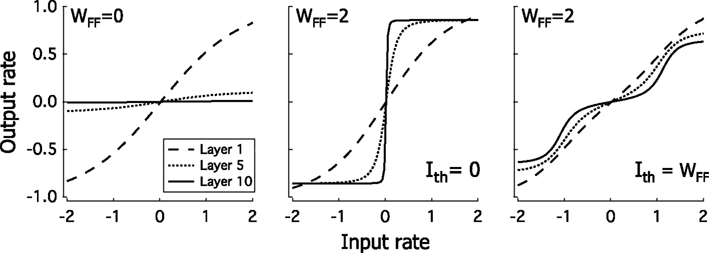
Figure 3. Response of the feedforward network when a spatially homogeneous input is applied. When W_FF is small the response is progressively weaker as ℓ is increased, so that for l = 10 the response is negligible. For large W_FF, the response in the last layer is close to a step from −1 to 1, for Ith = 0, while for Ith ≠ 0 it evolves to a 2 step response, from −1 to 0 at r₀ = −Ith/W_FF and from 0 to 1 at r₀ = Ith/W_FF.

To better understand this behavior we analyze the system near r₀ = 0. Since f (0) = 0 we have that if r₀ = 0, r_ℓ = 0 for all ℓ. For $0<r_0=\delta r_0\ll 1,$ r_ℓ = δr_ℓ is also much less than 1, and, to leading order, satisfies δr_ℓ = 2W_FFf ′(0)δr_{ℓ − 1} for l ≥ 1. Here f′ is the derivative of effective transfer function, f. This means that we can write δr_ℓ as δr_ℓ= Λ^ℓδ₀, where Λ = 2W_FFf ′(0). Thus, when |Λ| < 1 the response gets progressively smaller as ℓ is increased, while to |Λ| > 1 the size of the response increases with ℓ. Note that this decrease/increase is geometric, so that even for Λ relatively close to 1, δr_ℓ will deviate a lot from δr₀ for large ℓ. As a result, for Λ ≠ 1, at r₀ = 0, the slope of the function that plots r_ℓ against r₀ will be either very large or very small when ℓ is large.

Using equation (4) we have that $f^{\prime }\left(0\right)={\left[1+\text{cosh}\left(I\text{th}\right)\right]}^{-1}.$ If Ith = γW_FF, Λ is given by Λ = 2W_FF/[1 + cosh(γW_FF)]. For γ = 0, Λ = W_FF and, near r₀ = 0, the slope of the transfer is very low for W_FF < 1 for large ℓ, while for W_FF > 1 it becomes very steep. If γ > 0, Λ increases with W_FF for small W_FF, but it decreases asymptotically to 0 as W_FF is increased further and further. This is because for large W_FF, cosh(γW_FF) increases faster than W_FF. So as W_FF is increased from 0, Λ first increases from 0, until it reaches its maximum, then it decreases again to 0. The maximum value Λ takes depends on γ. If γ is to large, maximum value of Λ is less then 1, so that for large γ the slope of the transfer function near r₀ = 0 is small for any value of W_FF. This is demonstrated in Figure 4, where Λ is plotted against W_FF for different values of γ.

FIGURE 4

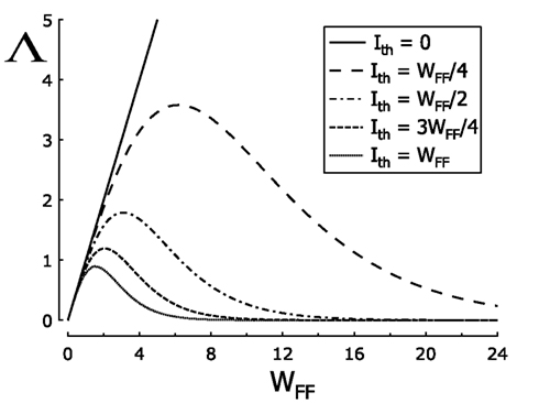
Figure 4. Behavior of the transmission slope, Λ, near the point 0 when strength W_FF increases. Different values of threshold, Ith are plotted to observe changes of firing rate transmission at large ℓ. At Ith = 0, the straight solid line crosses Λ = 1 only once, so the activity passes from low to high magnitudes in one transition. For other values of Ith, except for Ith = 1, curves cross twice the value Λ = 1. The range of these two intersection points in W_FF becomes shorter as curves Ith → W_FF. Thus, at large ℓ, firing rate decreases, increases, and again decreases as W_FF moves progressively to high values. When Ith = W_FF, the curve never crosses the values of Λ = 1, so any change in the transmission of the activity is observed around 0.

We will no examine the implications of these findings in the limit where the total number of layers L becomes infinite.

If we have a long chain of layers, the rates r_ℓ for large ℓ will approach a constant value. The values it can approach are the stable solutions of the equation r_∞ = f (2W_FFr_∞). With Ith = 0 one solution of this equation is r_∞ = 0, for any value of W_FF. For W_FF < 1 the curve of f will have a slope of less than 1 at r = 0, and r_∞ = 0 is a stable solution. It is also the only solution. For larger W_FF the slope at r = 0 is larger than 1 and there are two extra solutions, one with r_∞ < 0 and one with r_∞ > 0 (see Figure 3A). In this case the solution r_∞ = 0 is unstable, that is, if r₀ deviates slightly from 0, the deviation from this value increases as ℓ is increased. For an infinite chain of hierarchical levels, r_ℓ approaches one of the other two solutions with increasing ℓ. r_ℓ Goes to the smaller value if r₀ < 0, while it goes to the larger value for r₀ > 0. As show in Figure 5A, as W_FF in increased, the two stable non-zero solutions approach −1 and 1 respectively.

FIGURE 5

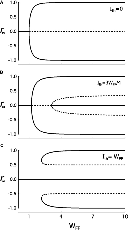
Figure 5. Fixed-points solutions, r_∞, are plotted as a function of increasing W_FF at three Ith values. Solid lines correspond to a stable and dashed line to an unstable solution. In (A), at Ith = 0 and W_FF = 1, the system undergoes a pitchfork bifurcation in which three solutions appear. The solution at r_∞ = 0 becomes unstable and the other two are stable. For (B,C), at Ith ≠ 0, the bifurcation point around r_∞ = 0 depends of f ′(0) = 2[W_FF/(1 + cosh(W_FF Ith))] while the critical point of bifurcation is no longer W_FF = 1. In (B), after the first bifurcation, a second pitchfork bifurcation appears when W_FF increases. The system has five final fixed-point solutions. Here, fixed-point that was unstable at r_∞ = 0 becomes stable, and two new unstable fixed-points emerge at ±γ/2. In (C), both previously described bifurcation have merged and from one stable solution the system passes suddenly to five final fixed-points as W_FF gradually increases.

When Ith = γ W_FF ≠ 0, the solution r_∞ = 0 also exists for all values of W_FF. However, the stability of this solution depends on γ. For sufficiently small γ there is a transition from a stable to an unstable solution, followed by a second transition from unstable to stable, as W_FF is increased. The first transition is the same as that for the case where Ith = 0. Below this transition r_∞ = 0 is a unique solution which is also stable. Above the transition two new stable solutions appear. These solutions approach −1 and 1 as W_FF is increased. The second transition is also a pitchfork bifurcation of the r_∞ = 0 solution. The r_∞ = 0 switches from unstable to stable and two more solutions appear. These are unstable and asymptotically approach the values ±γ/2. The value of W_FF at which the first bifurcation occurs increases with γ, from W_FF = 1, the bifurcations point of the Ith = 0 solution. The point where the second bifurcation occurs starts at W_FF → ∞ for γ → 0 and decreases with increasing γ. See Figure 5B.

These two critical values of W_FF converge in one bifurcation point as γ increases. We have observed that at the first transition point we move from 1 solution to 3 solutions. At the second, we move from 3 to 5 solutions. As γ is increased the separation between both bifurcation points becomes narrower and narrower. When distance between these two points reaches 0, both points converge turning out only one critical value. At this value we have a transition from 1 to 5 solutions. For still higher values of γ there no longer is a bifurcation from the solution r_∞ = 0, this solution stays stable. Instead at a critical value of W_FF two new pairs of solutions emerge. For r > 0 a stable solution with large r_∞ appears, together with an unstable solution that lies between this solution and the r_∞ = 0 solution. There is also a corresponding pair of solutions with r < 0. These solutions are shown in Figure 5C.

To obtain the regions that 1, 3, or 5 fixed-point solutions we determine the number of solutions in the plane (W_FF, γ). The transition from 1 solution to 3 solutions and from 3 to 5 solutions are the solutions of Λ = 1 with the smaller and larger solution respectively of W_FF at fixed γ. These are obtained by solving

$W_{FF}=\frac{\text{cosh}\left(\gamma W_{FF}\right)+1}{2}.$(20)

Taking the parametrization x = γ W_FF, this can be separated in a set of two equations:

$W_{FF}\left(x\right)=\frac{\text{cosh}\left(x\right)+1}{2},\gamma \left(x\right)=\frac{2x}{\text{cosh}\left(x\right)+1}.$(21)

Using this, we plot 1/W_FF against γ in relationship with the parameter x. Figure 6 shows the solutions of the purely feedforward model when a spatial homogeneous input is applied in layer 1. In the plane, the region for 1 solution is the only stable solution for W_FF small. As W_FF increases and γ is small, 3 solutions appear while two of them are stables. Holding the previous threshold condition and increasing W_FF even further, 5 solutions show up three stables fixed-points and 2 unstable ones. As γ is progressively increased to 1, the range over which there are 3 solutions shrinks. When γ ≈ 0.89 both boundaries are merged. For γ > 0.89 there is a transition from 1 solution to 5 solutions. This transition was determined from solving the fixed-point equations directly.

FIGURE 6

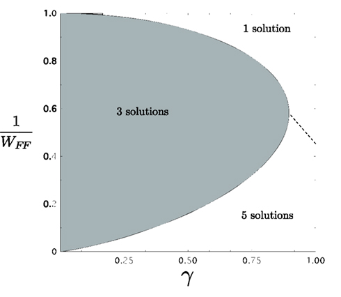
Figure 6. Number of solutions for the feedforward model as W_FF and γ are varied. 1, 3, and 5 fixed-point solutions appear in the plane as described in Figure 5. When W_FF ≤ 1 only one stable solutions is produced. In the plane, from 1 stable fixed-point solution, the system can pass directly to 3 or 5 fixed-point solutions as W_FF or γ change.

3.1.2. Model with feedforward and feedback connections

We now explore the effects of feedback connections when a homogeneous input is applied. As before $r_{k,i}^{\ell }=0$ for k ≥ 2 and we can write $r_{1,i}^{\ell }=r_{\ell }.$ In this case, the input for equation (1) have W_FB ≠ 0 and W_CP = 0. The new system is described by the equations

${\tau }_r\frac{d{r}_{\ell }}{dt}=-r_{\ell }+f\left(2W_{FF}{r}_{\ell -1}+W_{FB}{r}_{\ell +1}\right),l=1,...,L-1$(22)

and

${\tau }_r\frac{d{r}_L}{dt}=-r_L+f\left(\left[2W_{FF}+W_{FB}\right]r_{L-1}\right).$(23)

Effective W_FF values of the new system – The objective here is to analyze if the feedback connections improve the sequential transmission through the cortical hierarchy. As we know from the analytical results of the feedforward model there are two possibles final states. Here, we look for the influence of the factor W_FB on the behavior of this final states. We consider the system equations (22) and (23) in the steady state for a constant input, r₀

$r_{\ell }=f\left(2W_{FF}{r}_{\ell -1}+W_{FB}{r}_{\ell +1}\right),l=1,...,L-1$(24)

and

$r_L=f\left(\left[2W_{FF}+W_{FB}\right]r_{L-1}\right),$(25)

As before, for r₀ = 0 the solution is r_ℓ = 0. For small input r₀ = δr₀ we can expand the solution, and write

$\delta r_{\ell }=f^{\prime }\left(0\right)\left[2W_{FF}\delta r_{\ell -1}+W_{FB}\delta r_{\ell +1}\right],$(26)

and

$\delta r_L=f^{\prime }\left(0\right)\left[2W_{FF}+W_{FB}\right]\delta r_{L-1}.$(27)

Making the Ansatz δr_ℓ = Λ^ℓδr₀, we obtain from equation (26) that Λ has to satisfy

$\Lambda =f^{\prime }\left(0\right)\left[2W_{FF}+W_{FB}{\Lambda }^2\right],$(28)

which has the solutions Λ₊ and Λ₋. These solutions are given by

${\Lambda }_{\pm }=\frac{1}{2f^{\prime }\left(0\right)W_{FB}}\left[1\pm \sqrt{1-8{\left[f^{\prime }\left(0\right)\right]}^2{W}_{FF}{W}_{FB}}\right].$(29)

The general solution to the system can be written as

$\delta r_{\ell }=\left({\psi }_{+}{\Lambda }_{+}^{\ell }+{\psi }_{-}{\Lambda }_{-}^{\ell }\right)\delta r_0,$(30)

where ψ₊ and ψ₋ are two constants.

From boundary condition, equation (27) we obtain that

${\psi }_{-}{\Lambda }_{-}^L+{\psi }_{+}{\Lambda }_{+}^L=f^{\prime }\left(0\right)\left[2W_{FF}+W_{FB}\right]\left[{\psi }_{+}{\Lambda }_{+}^{L-1}+{\psi }_{-}{\Lambda }_{-}^{L-1}\right],$(31)

while from l = 0 we have ψ₊ + ψ₋ = 1.

After some algebra, one obtains that δr_ℓ is given by

$\delta r_{\ell }=\frac{{\Lambda }_{-}^{\ell }-\kappa {\Lambda }_{-}^L∕{\Lambda }_{+}^{L-\ell }}{1-\kappa {\Lambda }_{-}^L∕{\Lambda }_{+}^L}\delta r_0,$(32)

where κ = [1 – f ′(0)(2W_FF + W_FB)/Λ_]/[1 – f ′(0)(2W_FF + W_FB)/Λ₊]. If 8[f ′(0)]²W_FFW_FB < 1, |Λ₋/Λ₊| < 1, otherwise |Λ₋/Λ₊| = 1. So, in the large L limit $\delta r_L={\Lambda }_{-}^L\left[1-\kappa \right]∕\left[1-\kappa {\left({\Lambda }_{-}∕{\Lambda }_{+}\right)}^L\right]\delta r_0$ goes to zero in the large L limit, if |Λ₋| < 1, while for |Λ₋| > 1 δr_L becomes very large. The transition occurs when Λ₋ = 1, or f ′(0)[2W_FF + W_FB] = 1.

Let us now consider the behavior high up in the hierarchy when r₀ is not approximately 0. As in the network with only feedforward connections, for arbitrary r₀, r_ℓ will approach a set of fixed value as ℓ is increased. Here, these fixed values are the stable solutions of

$r_{\infty }=f\left(\left[2W_{FF}+W_{FB}\right]r_{\infty }\right).$(33)

Thus we can conclude that a network with feedback connections with strength W_FB and feedforward connections with strength W_FF, behaves very similarly to a purely feedforward network in which the strength is ${\tilde{W}}_{FF}=W_{FF}+W_{FB}/2.$ Both networks have the same fixed values to which the rates evolve as ℓ is increased, and if r₀ is small, for both the rate geometrically increases (decreases) when ${\tilde{W}}_{FF}<1\left(>1\right).$ Thus adding feedback connections does not qualitatively improve the ability of the network to have an output in the higher areas of the hierarchy that vary smoothly with r₀.

3.1.3. Feedforward and pulvinar model for a homogeneous input

We now consider the effect of adding a Pulvinar like structure (W_CP ≠ 0 and W_PC ≠ 0) on the response of the network to constant input, $r_i^0=r_0.$ To simplify the calculations we assume that there are no feedback connections (W_FB = 0). The model with feedback connections behaves qualitatively similar.

It is straightforward to verify that, as before, $r_{k,i}^{\ell }=0$ for k ≠ 1 and that $r_{1,i}^{\ell }=r_{\ell }.$ Likewise, for the Pulvinar we have that $s_{k,i}^{\ell }=0$ for k ≠ 1 and $s_{1,i}^{\ell }=s_{\ell }.$ Taking this into account, the equilibrium rates, r_ℓ and s_ℓ, are, for l = 1, 2, …, L, given by

$r_{\ell }=f_{ctx}\left(2W_{FF}{r}_{\ell -1}+W_{CP}{s}_{\ell -1}\right)s_{\ell }=f_{pul}\left(2W_{PC}{r}_{\ell }+J_{\ell }\right).$(34)

Here f_ctx and f_pul are the transfer functions of the cortical and Pulvinar units respectively, while s₀ = 0, J₁ = 0, J₂ = 2W_FPs₁, and J_ℓ = (2W_FPs_{ℓ − 1} + W_LPJ_{ℓ − 1})/(1 + W_LP).

Due to the parallel processing and long range connections, a full analysis of this system is much more involved that the analysis of the system without Pulvinar that we have analyzed above. This analysis is beyond the scope of this paper, here we will concentrate on the response of the system to small input, r₀ = δr₀ and indicate how the system behave differently from the network without Pulvinar.

If r₀ = δr₀ is small, the response of all layers of the cortex and Pulvinar will be small, r_ℓ = δr_ℓ and s_ℓ = δs_ℓ, with

$\delta r_{\ell }=F_{ctx}\left[2W_{FF}\delta r_{\ell -1}+2W_{CP}\delta s_{\ell -1}\right]\delta s_{\ell }=F_{pul}\left[2W_{PC}\delta r_{\ell }+\delta J_{\ell }\right],$(35)

where δJ_ℓ = (2W_PFδs_{ℓ − 1} + W_LPδJ_{ℓ − 1})/(1 + W_LP), $F_{ctx}=f_{ctx}^{\prime }\left(0\right)$ and $F_{pul}=f_{pul}^{\prime }\left(0\right)$.

Analogous to what happened in the cortical network with feedback we can here, for l ≥ 2, write $\delta r_{\ell }=\left({\psi }_{-}{\Lambda }_{-}^{\ell }+{\psi }_{+}{\Lambda }_{+}^{\ell }\right)\delta r_0.$ For δs_ℓ we have $\delta s_{\ell }=\left({\varphi }_{-}{\Lambda }_{-}^{\ell }+{\varphi }_{+}{\Lambda }_{+}^{\ell }\right)\delta r_0.$ After some tedious algebra one can show that if the largest of eigenvalues, Λ₊, is larger than 1, δr_L is much larger than δr₀, while if it is smaller, δr_L will be much smaller than δr₀. Thus for a gradual increase of r_L with r₀, Λ₊ should be close to 1.

The eigenvalues Λ₊ and Λ₋ can be found by making the Ansatz δx_ℓ = Λ^ℓδx₀, where x is r, s or J. Inserting this into equations (35) we obtain

$\begin{array}{llll}{\Lambda }^{\ell }\delta r_0& =F_{ctx}\left[2W_{FF}{\Lambda }^{\ell -1}\delta r_0+W_{CP}{\Lambda }^{\ell -1}\delta s_0\right],& & \\ {\Lambda }^{\ell }\delta s_0& =F_{pul}\left[2W_{PC}{\Lambda }^{\ell }\delta r_0+{\Lambda }^{\ell }\delta J_0\right],& & \text{(36)}\end{array}$

while from δJ_ℓ = (2W_PFδs_{ℓ − 1} + W_LPδJ_{ℓ − 1}) we obtain

${\Lambda }^{\ell }\delta J_0=\frac{1}{\left(1+W_{LP}\right)}\left(2{\Lambda }^{\ell -1}{W}_{FP}\delta s_0+{\Lambda }^{\ell -1}{W}_{LP}\delta J_0\right).$(37)

Solving these equations under the assumption δr₀ ≠ 0, we find that Λ satisfies the quadratic equation

$\begin{array}{llll}& {\Lambda }^2-\Lambda \left(2W_{FF}{F}_{ctx}+2B+\frac{W_{LP}+2F_{pul}{W}_{FP}}{W_{LP}+1}\right)& & \\ & +\frac{2F_{ctx}{W}_{FF}{W}_{LP}+2B{W}_{LP}+4F_{ctx}{F}_{pul}{W}_{FF}{W}_{FP}}{W_{LP}+1}=0& & \text{(38)}\end{array}$

where B = W_FFW_PCW_CPF_ctxF_pul. Thus Λ₊ and Λ₋ satisfy the equation

$\begin{array}{l}{\Lambda }_{\pm }=W_{FF}{F}_{ctx}+B+\frac{1/2+F_{pul}\frac{W_{FP}}{W_{LP}}}{1+\frac{1}{W_{LP}}}\\ \pm \sqrt{{\left(W_{FF}{F}_{ctx}+B-\frac{1/2+F_{pul}\frac{W_{FP}}{W_{LP}}}{1+\frac{1}{W_{LP}}}\right)}^2-\frac{4B{F}_{pul}\frac{W_{FP}}{W_{LP}}}{1+\frac{1}{W_{LP}}}.}\end{array}$(39)

It might seem that we have not gained much by adding the Pulvinar. As before we have 2 eigenvalues whose values depend on the network parameters, so it would seem that we again need fine-tuning of the parameters to get an output δr_L of the same order as δr₀. Like before, for these fine-tuned parameters we may obtain that r_L is comparable to r₀ for small r₀, but not if r₀ becomes larger.

However, this is not the case: If we take that $W_{LP}\gg 1$ the two eigenvalues satisfy Λ₊ ≈ 2F_ctxW_FF(1 + W_CPW_PCF_pul) and Λ₋ ≈ 1. Thus in this case δr_L is comparable to δr₀, provided that |Λ₊| < 1.

When the activity in area L is plotted as a function of the input, the best relation is one that show a smooth linear increment of firing rate when the contrast gradually increase. This relation in the feedforward-pulvinar model is observed when the relation δr_ℓ ≈ δr₀ is satisfied, so Λ = 1. Therefore, we require 1 = 2F_ctxW_FF(1 + W_CPW_PCF_pul) when W_LP is large with the constraint of an arbitrary W_FP < W_LP. Without loss of generality, we consider when $I_{th}^{cx}=0,$ so F_ctx = 1/2, and we plug this result in Λ₁ to obtain

${\left[W_{FF}\right]}_{cr}=\frac{1}{1+F_{pul}{W}_{CP}{W}_{PC}},$(40)

where [W_FF]_cr is the value of the cortical gain of the effective transfer function equation (2).

Analytical and Numerical results of the models – The analytical treatment has shown that the cortico-cortical and the cortico-pulvinar-cortical network behave differently when a spatially constant input is applied. In the case of the purely feedforward model, considering L large, the rate will approach r_∞ to fixed-point solutions depending of the value of the threshold and the gain, W_FF. In the unimodal transmission, Ith = 0, the solutions go to one stable rate to two stable and one unstable as one moves from small to large W_FF. This bifurcation also exists at the bimodal transmission, Ith ≠ 0, but here occurring twice as the gain is progressively increased given at the end 5 solutions, three of them stables and two unstable. If we plot r_∞ against r₀ at large W_FF in the bimodal transmission, a double step response appears while both inflections points will be at ±Ith_.

The meaning of these results is that for small W_FF when Ith = 0, the response, r_ℓ, always approaches 0 with increasing ℓ for any input r₀, while for large W_FF it approaches upper stable solution for r₀ > 0 and the lower one for r₀ < 0. For Ith ≠ 0, solutions approach similar as before, but for W_FF large 2 unstable fixed-points appears in r₀ = ±Ith/2 and the 2 stables responses move forward to r₀ = ±1. As Ith > 0.9, r_ℓ = 0 becomes stable and the other 4 solutions maintain the same previous stability. Thus, information about r₀ is lost in the higher areas for any value of W_FF either for Ith = 0 or otherwise.

Adding feedback connections only, W_FB ≠ 0 and W_CP = 0, does not qualitatively improve the situation. The bifurcation point is adjusted to [W_FF]_cr = 2/W_FF(2 + W_FB), but for a sufficiently large L we still have an almost constant output for small W_FF and a step or double step response for larger W_FF when Ith = 0 or Ith ≠ 0, respectively.

The response of the network to spatially constant input with the pulvinar included, W_CP ≠ 0 and W_PC ≠ 0, could also be treated analytically. One solution that will satisfy a smooth linear increment of firing rate when the contrast input gradually increases will show up. This relation in the feedforward-pulvinar model is observed when $W_{LP}\gg 1$ with the constraint W_FP < W_LP. At $I_{th}^{cx}=0,$ this process is satisfied as W_FF = 1/(1 + F_pulW_CPW_PC), where W_FF is the cortical gain and F_pul the derivative of the effective transfer function for the pulvinar. This improvement in the last area’s activity is because pulvinar area ℓ receives input from all lower areas and passes directly to higher areas. Because of these long range interactions, responses in the higher pulvinar regions may not tend to a bimodal output distribution. This will be confirmed by numerical simulations.

3.1.4. Optimization

In this part we investigate what are the values of parameters that better explain a smooth linear increment of firing rate at r_L when an input is gradually varied in contrast. The optimal output of layer L is one that spans largely the dynamic range of outputs and conserves as much as possible a linear relation with the input, r₀. In the simulations, when a homogeneous input −1, 1 is applied to the feedforward model, a large W_FF assures utilization of the whole dynamic range between –1 and 1, but yields an extremely non-linear curve. Instead, for small W_FF the curve that plots r_L against r₀ appears much more linear, but only covers a small part of the output range. So, to combine properly these two requirements we work out the entropy of the output distribution by assuming that the r₀ is distributed homogeneously between −1 and 1. The entropy is high both in the case where the input-output relation is linear and also when the output range is large (see Materials and Methods for the mathematical description).

We look for the parameters values that maximize the entropy of the rate distribution of the last layer. Because, most of the analytical treatment considered both unimodal and bimodal transmissions, we analyze separately the cases where Ith = 0 and Ith ≠ 0. Tables 1 and 2 recapitulate the results for the different models. We consider as networks the purely feedforward (FF), feedforward-feedback (FF-FB), feedforward-pulvinar (FF-Pul), and feedforward-feedback-pulvinar (FF-FB-Pul). The highest entropy is obtained for models that have Pul. The lowest entropy is observed for the purely feedforward model. However, qualitatively FF and FF-FB are almost the same for both Ith = 0 and Ith ≠ 0. In spite of the several results, for Ith = 0, FF-FB-Pul always was more informative than the feedforward and feedforward-feedback model. For Ith = 0, FF-Pul has this role. Figure 7 shows the output of the four models with the optimal parameters.

TABLE 1

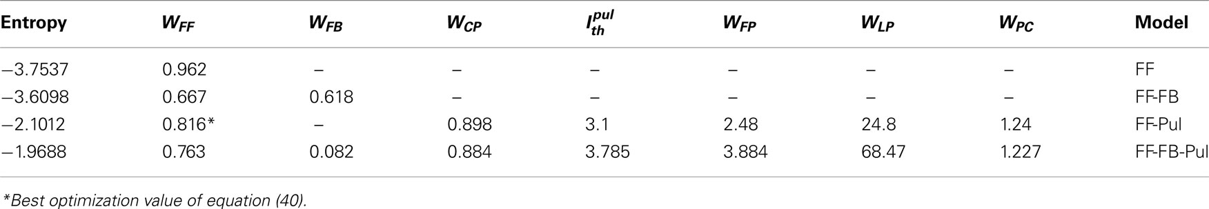
Table 1. Maximal entropy and optimal values of the network parameters with uniform input, when $I_{th}^{cx}=0,$ for network with only cortical feedforward connections (FF), cortical feedforward and feedback connections (FF-FB), cortical feedforward connections and pulvinar (FF-Pul), and full network (FF-FB-Pul).

TABLE 2

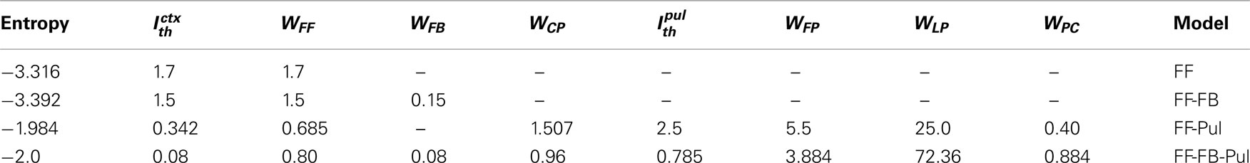
Table 2. Maximal entropy and optimal values of the network parameters for uniform input, when $I_{th}^{cx}\ne 0,$ for models as in Table 1.

FIGURE 7

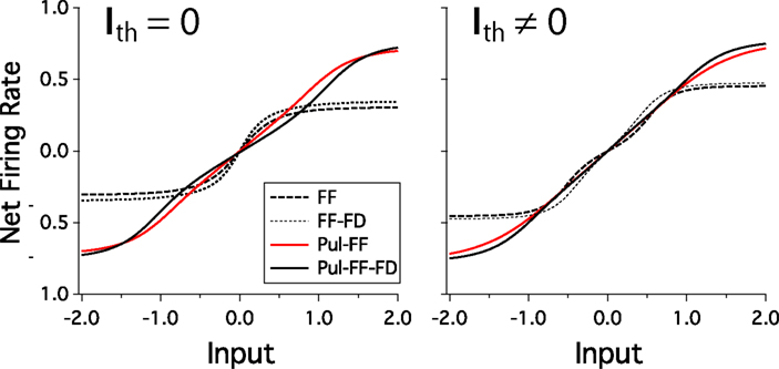
Figure 7. Net firing rate of last cortical area is plotted against increasing values of homogeneous spatial input for Ith = 0 (Left) and Ith ≠ 0 (Right). Here, best solutions for each model are plotted. Curves for feedforward (FF), feedforward and feedback (FF-FB), pulvinar-feedforward (FF-Pul), and pulvinar-feedforward-feedback (FF-FB-Pul) models. Parameter values are those from Tables 1 and 2.

Compare with the cortico-cortical networks, a smooth linear increase of firing rate is present when the Pul is included and almost the whole output range is used. For the FF-Pul model this solution is obtained when $W_{LP}\gg 1$ with W_FP < W_LP. For Ith = 0, W_FF was worked out with equation (40) and it was the best optimization value of the entire possibles values of variables analyzed (* in Table 1). To get these values for the networks with Pul, we also fit the reciprocal connections as W_CP > W_PC. Moreover, in the case of $I_{th}^{cx}\ne 0,$ W_CP were much stronger than that for the W_PC. However, without the reciprocal connectivity from the Pul the model present a low entropy finishing a constant rate in r^L. So that, the output for Pul models encodes optimally better an input than that for cortico-cortical networks.

3.2. Response to Visual Input

Now that we have analyzed the responses of the models with different architectures to a spatially constant input, $r_i^0=r_0,$ we are ready to explore the results when natural visual stimuli are applied. In modeling the response of the network to natural visual stimuli we take into account that for such stimuli the retina and LGN whitens the response and reduces the kurtosis of the distribution (Simoncelli and Olshausen, 2001). Thus visual input with natural statistics is, in our model, described by a random input, $r_i^0=\sigma x_i,$ where σ codes for the contrast and x_i is independently drawn from a Gaussian with mean 0 and variance 1. We assume that the same visual input with higher contrast is represented by an input with the same x_i but larger σ.

Before we study this case it is instructive to a simplified model in which the transfer function is linear, F(I) = I, and we have a purely feedforward cortical model. In the steady state, the firing rates of units in layer ℓ are given by $r_{k,2i-1}^{\ell }=W_{FF}\left[r_{2k-1,i}^{\ell -1}+r_{2k,i}^{\ell -1}\right]$ and $r_{k,2i}^{\ell }=W_{FF}\left[r_{2k-1,i}^{\ell -1}-r_{2k,i}^{\ell -1}\right]$. The output of the units in each layer are Gaussianly distributed and one easily shows that the mean is 0 and the variance satisfies $⟨{\left(r_{k,i}^{\ell }\right)}^2⟩={\left(2W_{FF}^2\right)}^{\ell }{\sigma }^2∕2$. Thus, while the random Gaussian activity moves step by step from lower to higher layers in the network, the variance of layer ℓ will always depend on the firing rate variance in ℓ − 1. When the feedforward strength has the value, $W_{FF}=W_{cr}\equiv 1∕\sqrt{2}$ the activity level is the same at all layers in the network. For W_FF < W_cr, $⟨{\left(r_{k,i}^{\ell }\right)}^2⟩$ decreases geometrically with ℓ. For W_FF > W_cr it increases geometrically. Thus, if L is large, the response in the last layer will be very large or very small unless W_FF is close to W_cr. On the other hand, because the whole system is linear if f (I) is linear, a change in contrast will rescale the response of all units in all layers by the same fraction, so that in each layer the response will be perfectly contrast invariant. This in the linear system the purely feedforward model gives us exactly what we want if we set W_FF = W_cr, we have contrast invariance of the tuning, information about the contrast in each layer and output can exploit the whole dynamic range.

3.2.1. Effects of the gain and threshold on the non-linear propagation of firing rate

In the network with a non-linear transfer function these requirements cannot be met exactly. In a purely feedforward model we can make the transfer function effectively linear by taking a small value of W_FF. This will ensure contrast invariance of the tuning, but in higher layers the response will by extremely small, so that, in the presence of noise a readout of the activity will give very little information about the stimulus. A larger W_FF will exploit the dynamic range of the system better, but introduces non-linearity in the response which may destroy the contrast invariance of the tuning and may make the contrast response function of the neurons in areas with large ℓ less smooth. A compromise between these two extremes needs to be made. We will now investigate how bad this compromise is in the purely feedforward cortical model and whether adding feedback connections and interactions with the pulvinar improves the network response.

3.2.2. Effects of feedforward strength and threshold on the non-linear propagation of activity

By assuming visual propagation in the feedforward network with a non-linear transfer function, f, the response of the system either decreases or increases with ℓ as the threshold, Ith, and the feedforward strength, W_FF, are varied. We investigate this sequential propagation quantifying the firing rate from layer 1 to L, using histograms of distribution at two values of contrast, σ = 0.1 and σ = 1.0. As a first approximation, we analyze the response of each layer with L = 10 keeping Ith constant and varying W_FF.

Independent of the contrast, the visual input passes through the layers like in the case of linear transmission. The response of layer L first decreases to zero, then blows as the strength, W_FF, is increased gradually from small to large values. For small W_FF, any given value of contrast produces firing rate distributions that progressively evolve from a broad to narrow distribution as l → L. The activity moving higher through the system stays in small region of the firing rate range surrounding the mean $⟨\left(r_{k,i}^{\ell }\right)⟩=0.$ As in the model with linear transfer function, the network integrates the visual input to a narrow distribution keeping only a small representation of the contrast. On the other hand, when W_FF is increased the network changes the modality of transmission. As W_FF becomes large, the rate distribution moves widens the range of activity and the distribution becomes multimodal as we move from layer to layer. As can be seen from Figure 8A at W_FF = 2, the distribution in the last layer is broad and unimodal for both low (σ = 0.1) and high (σ = 1.0) contrast. For larger W_FF, the distribution of the activity of units gradually becomes bimodal with peaks at the extrema of the response. At W_FF = 3, the visual input applied to l = 1 evolves sequentially through the network ending in net firing rates equal to –1 and 1 for most units. This tendency of the response to saturate at the borders is enhanced when W_FF becomes even larger. In each layer the activity moves progressively to r = −1 and r = 1 showing also a small peak around the value 0. Three clear solutions appear at W_FF ≤ 5. As we can see in Figure 8A at W_FF = 5, r¹ either starts with a broad distribution or already has net firing rates when a stimuli of low or high contrast is applied to the network. As the activity move from low to higher areas, large peaks are observed is at the maximum and minimum activity as well as a small cluster surrounding zero.

FIGURE 8

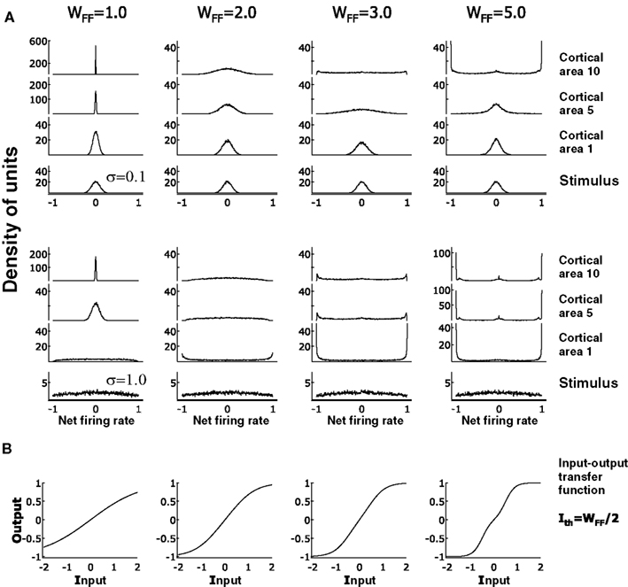
Figure 8. Propagation of activity through the feedforward network with increasing values of W_FF and a fix Ith. (A) Signal propagation is tested with low and high contrast and it is observed respectively in the top and the middle set of graphs. It can be seen that a low W_FF, any contrast input applied at area 1 produces a sharp response in last area. This response becomes broader for high and low contrast when W_FF = 2. A small transition is observed in early cortical areas in which two peaks at the borders of the distribution increase in number. At large values of W_FF, these peaks are more represented in the distribution of neurons. Given the shape of the input-output transfer function, at W_FF = 5, a small peak at net firing rate 0 appear, in addition to the peaks at the borders. (B) Input-output transfer functions at varied W_FF and Ith = W_FF/2. As in Figure 1, curves increase in non-linearity as W_FF also increases. Note when W_FF = 5, the double step shape in the curve produces a peak in the neuron distribution at the net firing rate 0. Density in arbitrary units.

The distribution of the activity in layer L can be one of types. For small W_FF the distribution is clustered around 0 for all contrast levels. For an intermediate strength the distribution is broad for large σ and narrower for smaller σ. Finally for large W_FF the distribution is multimodal for all contrasts with peaks near −1, 0, and 1. These results can be readily understood from the transfer function of the units shown in Figure 8B. Small W_FF corresponds to a transfer function f whose maximal slope is less then $1∕\sqrt{2},$ resulting in responses that get progressively small as ℓ is increased. For intermediate values the average slope is close to the critical value for a significant range of inputs. For large W_FF the gain is much larger than $1∕\sqrt{2}$ for a significant range around 0 and saturates at ±1 for larger values. This results in the outputs being pushed to the extrema as ℓ increases. The small peak near 0 in the output distribution can be understood from the fact that in the input we are summing two inputs from the previous layer. If these are at the extrema, but have opposite sign, the total input will be close to 0, resulting in a response of almost 0.

We now explore how the response of the network depends on the threshold. We determine the distribution of the activity in layer L. These distributions are shown in Figure 9. Here, we test the effect of varying W_FF for five different levels of Ith. In each case the distribution of the activity has been analyzed at two values of the contrast, σ = 0.1 and σ = 1.0. To make the presentation more clear, we discuss separately the results for Ith = 0 and for Ith ≠ 0.

FIGURE 9

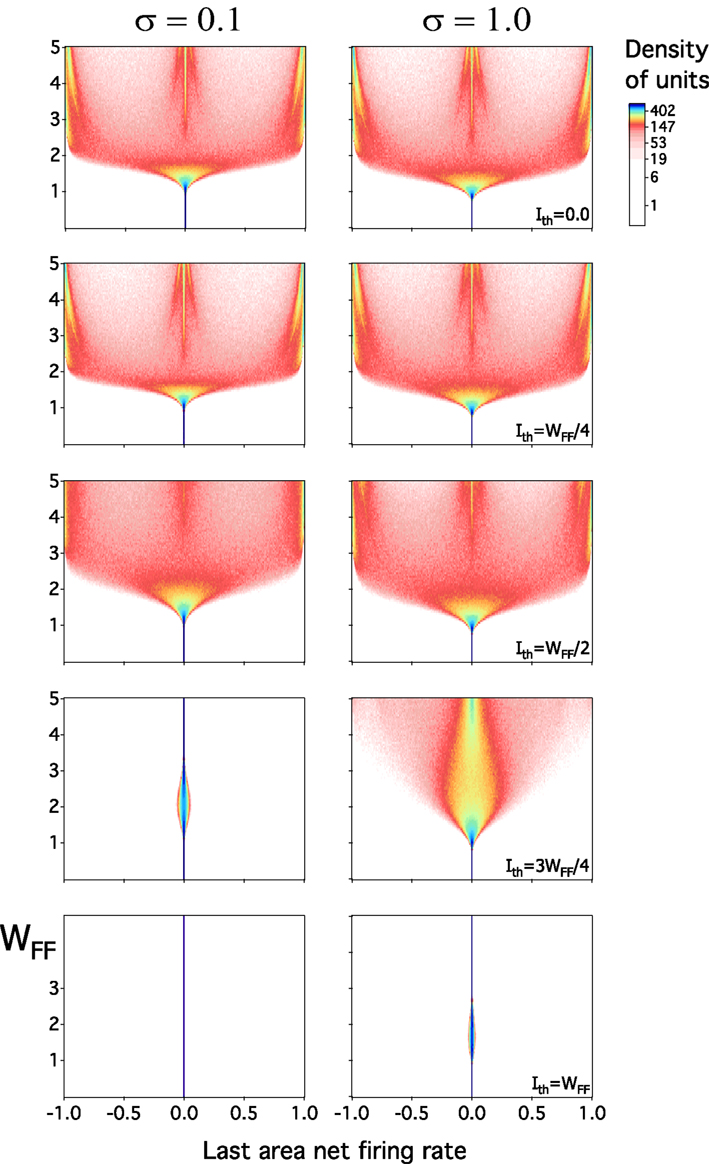
Figure 9. Activity of last layer in the feedforward model as W_FF is varied. Low and high contrast are tested at five values of Ith. Two gen Figeral patterns of activity appear as one moves Ith from small to large values. When Ith ≤ W_FF/2, activity is totally represented at 0 firing rate at small W_FF. As W_FF gradually increases, and around W_FF ≈ 1, the density of units becomes broader represented. A transition, near W_FF ≈ 2, emerges in which the density has an almost uniform distribution. This widening ends at larger values of W_FF, where activities are mostly at −1, 0, and 1. If W_FF → ∞, only these last three firing rates show up. This behavior is observed at low or high σ. Conversely, as Ith → W_FF, this expansion in the dynamic range progressively vanishes, and density of units is largely represented at 0. Density in arbitrary units.

From the linear feedforward network, the know that the activity collapses to 0 if the transfer function has a derivative at 0, which is less than $1∕\sqrt{2}.$ which means, for Ith = 0 that W_FF has to be larger than $\sqrt{2}$ to get a distribution with a finite width. This is confirmed in Figure 9. For W_FF less than approximately $\sqrt{2}$ the distribution is concentrated around 0. For larger values it is it is spread out and eventually becomes multimodal as explained above.

Now we analyze the layer L output when Ith ≠ 0. As in the previous case, the behavior of the system is pretty much the same on the interval 0 < Ith ≤ W_FF/2. The activity moves from one to three peaks at any value of contrast with a gradual transition between both extremes. As the threshold increases, qualitatively different behavior is observed. For σ = 0.1 the response is peaked around 0 for any value of W_FF. For σ = 1 the response distribution is broadened for W_FF > 1.4 when Ith = 3 W_FF/4, but this distribution narrows again for even larger values of W_FF. If we take Ith = W_FF, the output distribution is always narrow.

Why does the activity stays near 0 when Ith = W_FF? The assumption of a linear transfer function f produces a narrow distribution of rates in layer L for a small gain. For Ith ≠ 0, the function f always has a bimodal derivative as W_FF is sufficiently large, and the derivative near 0 becomes very small at 0. Thus for small inputs the response decreases as ℓ is increased. Whether there is a significant response for broader input distribution depends on whether a large enough fraction of the inputs is beyond the thresholds of the transfer function. For larger Ith are further apart so that is less likely that enough of the input exceeds the thresholds. Thus for Ith = 3W_FF/4 one can have a relatively broad output distribution for σ = 1, while for Ith = W_FF this is not the case.

3.2.3. Output response tuning

In the analysis of the feedforward network we observed that the firing rate of units in layer L, $r_{k,1}^L,$ stays near 0 when W_FF is small and approximately takes one of the three fixed solutions for large W_FF. In these cases the distribution of output rates is also nearly independent of σ. Only in a small range of W_FF the model shows a gradual variation of the distribution to changes in stimulus contrast. Adjusting the threshold does not produce any clear improvement. The respond of the feedforward model to variations in contrast is far from the desired result and we consider alternative network architectures to see whether they give an improvement. To do that we consider response $r_{k,i}^L$ of the last cortical area, when feedback connections and interaction with the pulvinar are included. Moreover, we will not only consider the amplitude of the response over the network, but will also consider contrast invariance of the tuning and the contrast response function of the units. Here we take contrast invariance of the tuning to mean that the input elicits in the last layer an output vector $r_{k,1}^L$ whose direction is independent of contrast. Smooth increase of the contrast response means that the length of this vector increases gradually with contrast. To account both these properties, we varied the optimization procedure used before for the spatially constant input.

To test whether the network response is sensitive to changes in contrast, we measure the response $r_{k,1}^L$ when the input standard deviation, σ, is now gradually changed. We estimate two properties of the output firing rate: The output amplitude is a function of the contrast and the mean angle between different values of contrast. The output amplitude, F, is defined as average length of the response of layer L for LGN inputs with widths σ, $F\left(\sigma \right)=⟨\left|\overrightarrow{\text{V}}\right|⟩$, where the average is over input patterns with standard deviation σ. We aim for an amplitude function F that is as linear as possible and uses the dynamic range maximally. We use H_L defined as $H_L={\int }_0^{1}d\sigma log\left(F^{\prime }\left(\sigma \right)\right)$ as the cost-function for this property. If H_L → L log2, the output scales linearly and exploits the whole dynamic ranges. It decreases if less of the dynamic range is used or the response is non-linearly. To explore whether the network can maintain contrast invariant tuning, we calculate the mean of distance S between normalizes output vectors $\overrightarrow{\text{e}}\left(\sigma \right)$ and $\overrightarrow{\text{e}}\left({\sigma }^{\prime }\right)$ for LGN inputs $r_i^0=\sigma x_k$ and $r_i^0={\sigma }^{\prime }{x}_k$ respectively, $S={\int }_0^{1}d\sigma {\int }_0^{1}d{\sigma }^{\prime }\overrightarrow{\text{e}}\left(\sigma \right)\cdot \overrightarrow{\text{e}}\left({\sigma }^{\prime }\right).$ Here $\overrightarrow{\text{e}}=\overrightarrow{\text{V}}∕\left|\right|\overrightarrow{\text{V}}\left|\right|.$ If S = 1 then vectors are in the same direction for all contrasts. As the direction changes more with contrast, S decreases. We define an error $E=-2S-e^{H_L}$ that takes both these factors into account.

For networks with different architectures we determine the parameters which minimize the cost function E. We analyze separately when Ith = 0 and Ith ≠ 0. To optimize each network we have used Powell’s method in multiple dimensions (Press et al., 1992). Tables 3 and 4 show the results for the different models. We consider same systems from the homogeneous spatial input analysis, but considering more cases for Ith = 0. First in models which Ith = 0, we observe that the best minimization is produced by the network FF-FB-Pul with threshold for both cortex and Pul $I_{th}^{ctx,pul}=0.$ The less improvement is for FF, nevertheless this network presents the best S value. Between these values, models that have both Ith = 0 are better than those that have only the $I_{th}^{ctx}=0.$ Thus, for the cost function E, ${\text{FF}}_{I_{\text{th}}=0}{\text{-FB-Pul}}_{I_{\text{th}}=0}<{\text{FF}}_{I_{\text{th}}=0}{\text{-Pul}}_{I_{\text{th}}=0}<{\text{FF}}_{I_{\text{th}}=0}\text{-FB-Pul}<{\text{FF}}_{I_{\text{th}}=0}\text{-FB-Pul}<\text{FF-FB}<\text{FF}$. It is surprising that the network with $I_{th}^{ctx,pul}=0$ has an optimal enough minimization of E that it approaches the value for networks with Ith ≠ 0. The model with $I_{th}^{ctx,pul}=0$ does better in S but the range of magnitudes is smaller. It seems that the action of a shortcut between low and high cortical levels overcomes partly the problem of non-linearity regardless the presence of a threshold. For cases with Ith ≠ 0, the model that minimize the cost function better is the FF-FB-Pul network, while the purely feedforward system has the least optimization. However, models with feedback do not qualitatively change the cost, compared to those without feedback. For example, the system FF-FB-Pul has a small negative value of W_FB and its presence produces only a slight improvement in S. Indeed, networks with feedback input tend to converge toward small negative values, except for FF-FB. Here, the feedback input produces a slight improvement in the H_L and keeps almost the same value of S. For these networks, the cost function E is FF-FB-Pul < FF-Pul < FF-FB < FF.

TABLE 3

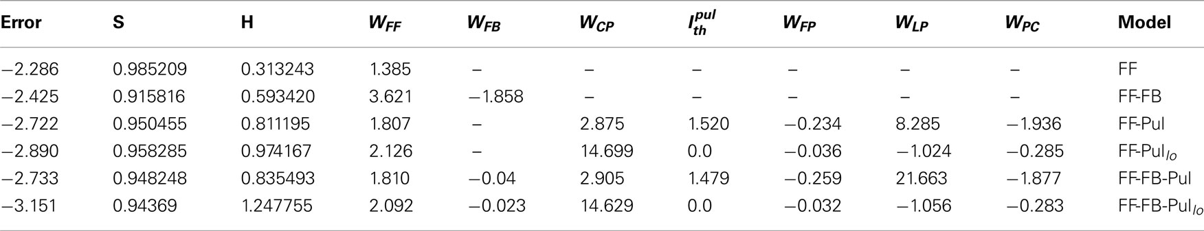
Table 3. Minimal error and optimal values of the parameters for visual input in the when $I_{th}^{cx}=0.$ Models as in Table 1.

TABLE 4

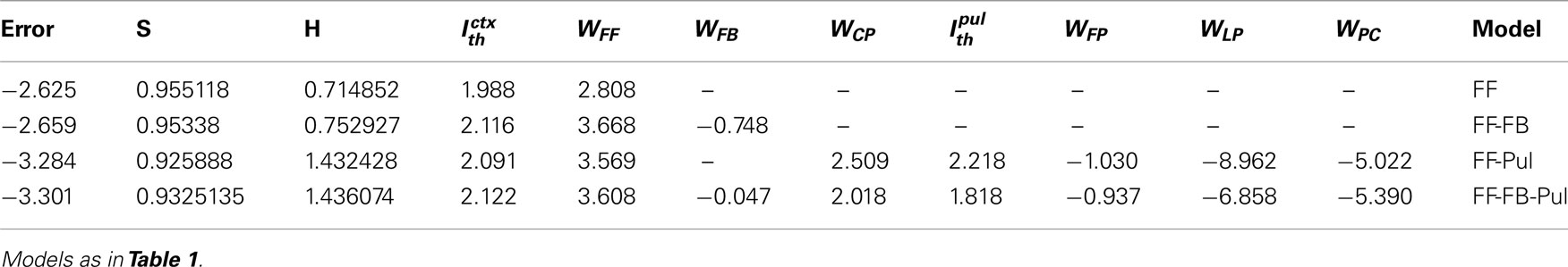
Table 4. Minimal error and optimal values of the parameters for visual input in the when $I_{th}^{cx}\ne 0.$

To graphically observe how the networks optimize this error we plot the response of a neuron at contrast σ varied against the response of the same cell at contrast σ = 1. Only feedforward (Figure 10 Left) and feedforward-pulvinar networks (Figure 10 Right) are plotted. For both architectures the contrast invariance of the tuning reasonable good, as reflected by the fact that the points fall nearly on a straight line. However, for the feedforward the slope of this line does not change much as σ is varied, reflecting the fact that the response amplitude only changes weakly with the contrast. Furthermore the dynamic range is not fully used here.

FIGURE 10

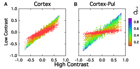
Figure 10. Response to different contrast for models FF (Left) and FF-Pul (Right) for $I_{th}^{cx}=0$ . Response of last cortical activity is represented by scatter-plot at contrast σ which is plotted against the same last cortical response at highest contrast, σ = 1. Scatter-plot of different colors represent 10 levels of contrast σ (From 0.1 to 1 at steps of 0.1). Values used are those from Table 3.

In the cortico-pulvinar-cortical model the dynamical range is almost fully exploited and the response amplitude increases by almost a factor of 5 as the contrast is increased from σ = 0.1 to σ = 1. This is further illustrated in Figure 11. In Figure 11A we plot the average response amplitude against the contrast for both architectures. In Figure 11B the separation between the normalized response vector for contrast σ and the normalized response vector averaged over contrasts, is plotted against σ with Ith = 0 and Ith ≠ 0. For both models S varies over the range 0.99 to 0.93, but the response amplitude clearly increases more linearly and uses more of the dynamic range for the cortico-pulvinar-cortical model. When Ith = 0, the separation response is better for the FF network followed for the FF-FB system. The inclusion of Pul to those system produces a sharp tuning of the separation response while for both low and high contrast the amplitude decreases. For the case Ith ≠ 0, is clearly that the small negative feedback input produces a shift of the average response curve to the right, producing a more linear output in the FF-FB-Pul system. However, compare to the FF-Pul network, the separation response decreases in amplitude as a function of the contrast. Systems without Pul present a wider and higher tuning (separation) response to contrast, but differences in magnitude are qualitatively similar. So that, systems with Pul included always show a less cost function while the improvement is produced overall for an enlargement of the length response as a function of contrast. In almost all the cases, this improvement occurs as $\left|W_{LP}\right|\gg 1$ and |W_FP| < |W_LP|.

FIGURE 11

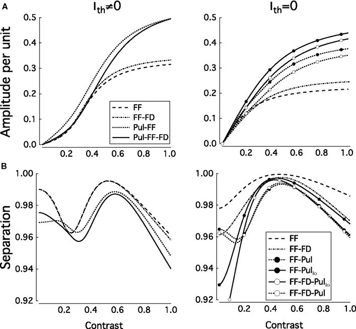
Figure 11. (A) Average response amplitude per unit (R) against the contrast and separation between the normalized response vector for contrast σ and (B) the normalized response vector averaged over contrasts (S), against σ. Values used are those from Table 4. Total number of simulations, 200. FF, feedforward; FF-FB, feedforward and feedback; FF-FB-Pul, feedforward, feedback, and pulvinar networks. The subscript Io represents structure of the network with Ith = 0.

A recent work of Theyel et al. (2010) has shown that higher-order thalamic nuclei can drive the activity of cortex. With the optimization procedure we show that the best values are for the model with Pul-Cortex while |W_CP| > |W_PC|. A problem with the optimization analysis however is that we regard of qualitatively other good solutions that satisfy for a sufficient transmission. Then, models that included Pulvinar input can display another optimization when |W_CP| < |W_PC| or |W_CP| > |W_PC|. Thus, we investigate a simple case for the feedforward-pulvinar network when W_FF = W_FP and $I_{th}^{cx}=I_{th}^{Pul},$ and vary gradually W_CP and W_PC to observe whether exist more than a solution. As we can see in Figure 12 solutions that minimize the cost function of the network appear as a |W_CP|/|W_PC| ratio. We observe that an improvement is present when connections from cortex to pulvinar are negative (positive) while connections from pulvinar to cortex are positive (negative). Surprisingly there are at least two almost equally good solutions: in one |W_CP| is large and |W_PC| small. In the other |W_PC| is large and |W_CP| small. Our model does well when the cortex modulates the pulvinar while the pulvinar drives the cortex, but it does equally well when it is the other way around.

FIGURE 12

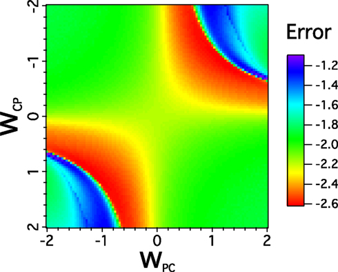
Figure 12. Representative behavior of the Pul-FFN network for varied W_CP and W_PC. The average error response is plotted to show an almost symmetrical response of the network as W_CP (W_PC) moves from positive to negative and W_CP (W_PC) goes from negative to positive values. The Pul-FF network is analyzed with W_FF = W_FP = 2.0, $I_{th}^{ctx}=I_{th}^{Pul}$ = 0.5, γ = 0, W_LP = 9, and W_FP = 0.

4. Discussion

The areas in the visual cortex are organized hierarchically and it is assumed that the arrangement of feedforward connections, together with recurrent inputs, is responsible for the increase in complexity and size of the receptive fields of neurons as one move up in this hierarchy. The visual areas in the cortex project to, and receive input from the pulvinar nucleus of the thalamus (Pul). Currently the role of Pul in the processing of visual information is not known.

We have explored the hypothesis that Pul is necessary to transmit information about the contrast of the visual scene to higher cortical areas. To test this hypothesis we constructed a simplified model of a path in the cortical hierarchy and connected this to simplified Pul model. The cortical hierarchy consists of L layers, each of which has 2^L populations of neurons, which are described by a rate model. In each layer of the hierarchy units receive feedforward input from 2 units in the preceding layer, in such a way that the RFs increase in size and complexity as one ascends the hierarchy. In agreement with experiments in primates (Shipp, 2001, 2003), Pul is also hierarchically organized and has similar RFs as the cortex. Cortical units in layer ℓ receive input from Pul units is layer ℓ − 1, while they send input to Pul units in layer ℓ. However, unlike in cortex, there are long range connections in Pul. Pul units in layer ℓ do not only receive feedforward inputs from units in layer ℓ − 1, but also from units in layers 1, 2, …, ℓ − 2.

In our model the cortical network by itself can manage complex receptive fields in the higher cortical areas, with contrast independent tuning, but only at the cost of weak sensitivity to contrast in the response of the higher layers. This is due to the non-linear transfer function of the cortical populations. The non-linearity of the transfer function will tend to make the output tuning of each population contrast dependent and this contrast dependence will tend to build up as the response moves up the hierarchy. Only by using a rather small fraction of the dynamic range of the population, over which the transfer function is approximately linear, can the tuning of the response in the higher cortical areas have approximately contrast independent tuning.

Adding a Pul to the system increases the capacity to code for contrast in higher cortical levels, without destroying the complexity of the RFs and compromising the contrast independence of the tuning. How is this achieved? In an early work, Bender has shown that lesions in striate cortex of macaque eliminates the visual response of pulvinar neurons (Bender, 1983). This and other experiments in the same direction (Bender and Butter, 1987; Chalupa, 1991; Casanova et al., 1997) suggest that striate cortex is necessary to establish the retinotopic map response in Pul. This is reflected in the topographical cortex to Pul connections in our model. Our assumption is that the Pul to cortex connections are similarly well organized. This explains why connecting our model of the visual cortical hierarchy to a Pul like structure does not interfere with the tuning properties of the RFs in the cortex. On the other hand, because of the long range interactions in Pul, the graded response with contrast in the first layer of Pul is transmitted all the way up to the highest layer. Because of the connection from this layer to the highest cortical layer, the input in the latter, and hence its response, is graded with contrast. This explains how contrast invariance of complex RFs in higher cortical areas can coexist with a graded response when a Pul is present.

It has been reported that RFs of pulvinar neurons have different visual properties that resemble those of cortical rather than subcortical neurons. As we have previously shown, that is due to the fact that pulvinar neurons are driven by visual cortical activity. Despite that the characterization of RFs in monkey are before the definition of classical cytoarchitectonic regions, RFs of cells in the inferior unit are discrete (1°–5° in the inferior pulvinar; Bender, 1982), and they are activated by simple visual stimuli. Similar to activation of cortical RFs, RF properties of pulvinar neurons have shown orientation and binocular selectivity, while a subset of neurons are direction selective (Bender, 1982). However, pulvinar RFs show a pronounced variability in their response compared to cortical RFs. Color-sensitive neurons are also found in lateral pulvinar (Felsten et al., 1983). Given these visual properties, it has been argued that RFs of pulvinar neurons resemble those of complex cells in the visual cortex (Casanova, 2003). This is reflected in our model. These types of RFs used are k = 1, 2. The more complex RFs, k = 2^{ℓ − 1}, 2^ℓ, are arbitrary defined. However, not much about more complex RFs in the Pul has been found. While the implement of different types RFs would not change the propagation of activity through the cortex, RFs from the Pul to the cortex have to respect the topography of the projection. That is, RFs from the Pul to cortex have to be similar in type. If the Pul network has more types of RFs the firing rate propagation in the cortex becomes even more linear. The perfect transmission will be when cortex and Pul have the same configuration of RFs from layer 1 to ℓ − 1.

For substantial improvement in the contrast sensitivity of higher cortical layers, the interaction between cortex and Pul needs to be substantial. Much experimental evidence shows that Pul, and in general higher-order thalamic nuclei, has a strong effect on neuronal activity in cortical areas. In a recent paper Logothetis et al. (2010), have shown that stimulation of Pul and not of LGN produces the activation of several cortical areas. Therefore, Pul should be involved overall in maintaining a stable firing rate while the feedforward cortical connections would determine which are the pathways that the transmission has to follow. By this assumption, for example, the Pul-effect observed in attentional task might be to increase the “salience” of visual objects that are mapped in the topographical visual cortex (Casanova, 2003; Shipp, 2004).

In our model the gradual increase with contrast of the response in higher cortical areas crucially depends on the shortcut provided by Pul. This shortcut is due to the explicit existence of long range interactions in the Pul. Experimental evidence support the long range connections. Long range interneurons have been described in the posterior portion of the medial pulvinar (PM; Imura and Rockland, 2006). These interneurons have widespread axon that extend at least 2.0 mm from its origin connecting different pulvinar portions (Imura and Rockland, 2007). Furthermore, it has been shown that these interneurons label for Parvalbumin (PV) and GABA. Remarkably, in the optimization procedure we have found that strengths for the long range interactions in Pul that minimize the error are negative. Despite the fact that our model is a simplification of the pulvinar architecture, and maybe long range interneurons lack a hierarchical organization, our assumption of negative long connections is in agreement with experimental data and the function of these long range connections could modulate and reach cells located in neighboring subdivisions.

It should be noted that in our model the cortical hierarchy needs to interact with the Pul, because the visual cortical hierarchy has many layers and effects of the non-linear transfer function accumulate as the response traverses more and more layers. In a visual cortex with only a few layers in the hierarchy, the CRF in the cortex can easily be smooth throughout the hierarchy without long range connections in the Pul. In this context it is in interesting to note that long range interneurons have been identified in the Pul of primates, but have not yet been identified in Pul of animals with a much simpler organization of their visual cortex. For example, that could be the case in the mouse in which the pulvinar is less denoted (Cajal, 1995) and the solution to solve visual transmission could be the direct connection from V1 to all visual areas (Wang et al., 2012). It is also noteworthy that in our model with 10 levels in the hierarchy, there are two choices for the connection parameters that are both close to optimal, for our optimization criterion. In one the feedforward connections in the cortex are strong and the pulvinar feedback to cortex is relatively weak. Here the cortical feedforward connections act as the driver and the pulvinar input as a modulator. In the second the connections from pulvinar to cortex are strong and the cortical feedforward connections are relatively weak. The pulvinar acts as the driver, while the cortical feedforward pathway can be considered as a modulator. Thus with respect to our optimization criterion both these theoretical options are equivalent (Sherman, 2007).

So far we have interpreted the negative long range interaction in Pul as the effect of long range inhibitory interneurons in Pul. However, these long range interactions could also be seen as an effective description of the interactions between Pul and other nuclei in the thalamus, which we do not incorporate in our model. Inhibitory inputs to Pul from the nucleus reticularis thalami (nRT) are a candidate (Sherman and Guillery, 2000). Another possible source of inhibition which has been observed recently is the input from two subcortical structures: the anterior pretectal nucleus (APT) and zona incerta (ZI; Lavallee et al., 2005). In the case of APT, this extrareticular pathway produce a powerful GABAergic afferent projections to posterior thalamic nuclear group (Po), a higher-order nucleus. This projection controls the neural activity, gating burst firing in Po neurons. In our model, a burst activity of Pul cell populations may be seen in the input-out transfer function when a large gain is used. In the optimization procedure for a spatial uniform input, either at Ith = 0 or Ith ≠ 0, the value of W_FP is larger than the cortical gain, W_FF, suggesting that Pul firing rate has a more step-like activity than cortical neurons as the input is applied. This evidence to observe sustained burst activity is also supported for extracellular recording of pulvinar neurons in monkeys during a visual fixation task (Ramcharan et al., 2005). On the other hand, the same group of authors have shown that the ZI inhibitory projection to the thalamus influences the discharge of Po cells negatively. This feedforward interaction will produce an inhibition of neural activity impeding sensory transmission. They also suggested that activity of Po neurons is mediated by a top-down disinhibition as the layer 5 cortical projections activate populations of ZI neurons. In our model, this mechanism may be captured effectively by the inhibitory projection of cortex to Pul that disinhibition the long range and feedforward connection. Recently, (Imura and Rockland, 2007) have found giant pulvino-cortical neurons which maybe are non-reciprocally projecting to their cortical targets as in a one-way mode. To these giant cells the presence of PV stain terminals was detected. Although the origin of the inhibitory connectivity remains uncertain, ZI and APT are good candidates for this afferent.

Another property of cortico-pulvino-cortical interactions is the non-reciprocal connectivity between cortex and Pul. Non-reciprocal connections appear as a key component of higher-order thalamic nuclei (Sherman, 2007; Llano and Sherman, 2008; Theyel et al., 2010). These interactions between cortex and thalamus have been described in different thalamic nuclei and the prime property would be to link two or more separate cortical areas. In our model, our assumption of non-reciprocal connectivity is based overall from the literature of cortex and Pul anatomical projections: cortical area ℓ + 1 receives both activity from cortical area ℓ and pulvinar area ℓ. For the effects of a feedforward communication pathway, we have considered that two neighboring cortical areas share a common pulvinar unit while the activity travels in a sequential manner throughout the cortex and Pul networks. However, also other types of connections would be included in our model. Reciprocal connections from Pul to cortex, similar to the connectivity from LGN to cortex (Sherman, 2007), and the possibility that pulvinar area ℓ = 1 could connect directly either several cortical areas at the same or the highest cortical area of the hierarchy (Rockland et al., 1999). In the case of reciprocal connections between Pul and cortex, in a recent work (Logothetis et al., 2010) report that electrical stimulation of Pul generates activation of V1 neurons, among other cortical areas. In our model, the implementation of these connections from higher to lower levels through the Pul would result in an even better input-output response. The activity from higher cortical areas could regulate down the activity on low levels similarly as the feedforward-pulvinar shortcut is acting in our simulations from lower to higher cortical areas (Cortes, 2008). On the other hand, non-specific connectivity from Pul to cortex also could improve transmission through the cortex. Our model, with only connections from Pul layer ℓ − 1 to cortical layer ℓ may therefore be unnecessarily restrictive. Clearly allowing also for connections to higher cortical layers would improve the contrast sensitivity in cortex.

There is some evidence that the Pul has a hierarchical and topographical organization. Based on cortico-thalamic and thalamo-cortical connections, (Shipp, 2003) postulates the existence of a “cortical gradient” inside the Pul, which the fronto-occipital axis in the cortex is reproduced as a medio-lateral gradient in the pulvinar (medio-lateral cortical axis rotates to a rostro-caudal gradient in the thalamus). Two connectivity examples clarify this idea. Injections with dual tracer in V1 and V4 label preferentially respective medio-caudal and latero-rostral pulvinar areas. This projecting gradient is also supported by injection in V2 (lateral within Pul) and inferior temporal areas (TEO, TF, TE; medial within Pul). On the other hand, injections in area V1, that represent retinotopic position of either the upper and lower contralateral hemivisual field, label neurons in respective hemield of both the lateral (PL) and inferior (PI) subdivisions. Two topographic map are present within the Pul. Bender (1981), with extracellular recording show that this retinotopically organized areas traverse the PL and PI. The representation through the pulvinar areas contains a complete map of the contralateral hemield of the monkey eye visual field. One representation lies mainly within the PI extending somewhat into the adjacent PL. The second lies entirely in the PL ending in the ventrolateral nucleus of PL (PLvl). The upper hemield of both areas are represented in the more ventral part of the Pul, whereas the lower is located upwards (Kaas and Lyon, 2007). Shipp (2003) have also postulated that these two maps found in the Pul topologically reproduce those from V1 and V2. This author argued that there is a preservation of cortical topography and topology (at least of V1 and V2), while 1° and 2° pulvinar maps are linear and parallel and they adopt a rostrolateralcaudo-medial alignment instead that a ventro-dorsal localization. Under this scope, our Pul-cortex model is quite similar to these anatomical evidences: the Pul conserves and transmits information overall from low cortical levels, and it connects with a hierarchical gradient the cortical arrangement.

Recent work has shown that connectivity of two neighboring cortical areas between which the communication is eliminated by cutting cortico-cortical connections are driven by higher-order thalamic nuclei (Theyel et al., 2010). Although the best value in the optimization procedure of our Pul-cortex model is when cortico-pulvinar connections are stronger than pulvino-cortical ones, there exists a qualitatively equal response when it is in the other direction. At the best value of optimization, we have also observed that there is a region of good values for |W_PC| > |W_CP|, when they are almost similar |W_CP| ≈ |W_PC|. This phenomenon to observe either |W_PC| > |W_CP| or |W_PC| ≤ |W_CP|, is emphasized when we simulated a equal network for Pul and cortex which parameters have the same parameters with W_LP = 9 and W_FP = 0. Here, solutions are symmetrical and either cortex can drive Pul or Pul can drive cortex. In the case of the best optimization, if there is some firing rate influence between both structure the weight of the connections presented should be very high. Maybe, the existence of this high interaction is due to the lack of reciprocal connections between Pul and cortex and both structures have to be in balance to compensate the existence of a coherence activity. In the same direction, the result that we have observed when positive (negative) and negative (positive) respectively cortico-pulvino and pulvino-cortical interactions are symmetrical suggest a balance state between both structures (Sherman and Guillery, 1998, 2011). Despite the fact that anatomical data in both pulvino-cortical and cortico-pulvinar projections of primates is not very extended, our result may clarify that in some cognitive task, i.e., attentional processes, Pul is activated and it can drive cortical activity. Perhaps, the effective connectivity of the Pul-cortex network is in a driver/modulator ratio while both solutions are possible because the different cognitive states of the subjects analyzed. The Pul-cortex network may switch dynamically in these two states, driver/modulator, without alternate the transmission of activity through the cortex. More details theoretical works have to be done for explain better the dynamic of the cortico-pulvino and pulvino-cortical projections, including for example the nature of the different cortico-pulvino terminals observed (Rockland, 1996) and the burst activity of pulvinar neurons (Ramcharan et al., 2005).

Conflict of Interest Statement

The authors declare that the research was conducted in the absence of any commercial or financial relationships that could be construed as a potential conflict of interest.

References

Albrecht, D., and Hamilton, D. (1982). Striate cortex of monkey and cat – contrast response function. J. Neurophysiol. 48, 217–237.

Pubmed Abstract | Pubmed Full Text

Avidan, G., Harel, M., Hendler, T., Ben-Bashat, D., Zohary, E., and Malach, R. (2002). Contrast sensitivity in human visual areas and its relationship to object recognition. J. Neurophysiol. 87, 3102–3116.

Pubmed Abstract | Pubmed Full Text

Baylis, G., Rolls, E., and Leonard, C. (1985). Selectivity between faces in the responses of a population of neurons in the cortex in the superior temporal sulcus of the monkey. Brain Res. 342, 91–102.

Pubmed Abstract | Pubmed Full Text | CrossRef Full Text

Bender, D. (1981). Retinotopic organization of macaque pulvinar. J. Neurophysiol. 46, 672–693.

Pubmed Abstract | Pubmed Full Text

Bender, D. (1982). Receptive-field properties of neurons in the macaque inferior pulvinar. J. Neurophysiol. 48, 1–17.

Pubmed Abstract | Pubmed Full Text

Bender, D. (1983). Visual activation of neurons in the primate pulvinar depends on cortex but not colliculus. Brain Res. 279, 258–261.

Pubmed Abstract | Pubmed Full Text | CrossRef Full Text

Bender, D., and Butter, C. (1987). Comparison of the effects of superior colliculus and pulvinar lesions on visual-search and tachistoscopic pattern-discrimination in monkeys. Exp. Brain Res. 69, 140–154.

Pubmed Abstract | Pubmed Full Text | CrossRef Full Text

Bullier, J. (2003). “Hierarchies of cortical areas,” The Primate Visual System, In eds J. Kaas, and C. Collins (Boca Raton, FL: CRC Press), 181–204.

Cajal, R. S. (1995). Histology of the Nervous System of Man and Vertebrates (History of Neuroscience, No 6) (2 Volume Set). Oxford: Oxford University Press.

Casanova, C. (2003). “The visual functions of the pulvinar,” in The Visual Neurosciences, eds L. Chalupa, and J. Werner (London: The MIT Press), 592–680.

Casanova, C., Savard, T., and Darveau, S. (1997). Contribution of area 17 to cell responses in the striate-recipient zone of the cat’s lateral posterior-pulvinar complex. Eur. J. Neurosci. 9, 1026–1036.

Pubmed Abstract | Pubmed Full Text | CrossRef Full Text

Chalupa, L. (1991). “Visual function of the pulvinar, in vision and visual dysfunction,” in The Neural Basis of Visual Function, eds B. Dreher, and S. Robinson (Boca Raton: CRC Press), 140–159.

Cortes, N. (2008). Le rôle de la boucle cortico-pulvinar-cortical dans la transmission dinformation. Master’s thesis Research in Cognitive Sciences. École des hautes études en sciences sociales (EHESS). Paris, France.

Felleman, D. J., and Van essen, D. C. (1991). Distributed hierarchical processing in the primate cerebral cortex. Cereb. Cortex 1, 1–47.

Pubmed Abstract | Pubmed Full Text | CrossRef Full Text

Felsten, G., Benevento, L., and Burman, D. (1983). Opponent-color responses in macaque extrageniculate visual pathways – the lateral pulvinar. Brain Res. 288, 363–367.

Pubmed Abstract | Pubmed Full Text | CrossRef Full Text

Hegdé, J., and Felleman, D. J. (2007). Reappraising the functional implications of the primate visual anatomical hierarchy. Neuroscientist 13, 416–421.

Pubmed Abstract | Pubmed Full Text | CrossRef Full Text

Imura, K., and Rockland, K. (2006). Long-range interneurons within the medial pulvinar nucleus of macaque monkeys. J. Comp. Neurol. 498, 649–666.

Pubmed Abstract | Pubmed Full Text | CrossRef Full Text

Imura, K., and Rockland, K. (2007). Giant neurons in the macaque pulvinar: a distinct relay subpopulation. Front. Neuroanat. 1:2.

CrossRef Full Text

Kaas, J. H., and Lyon, D. C. (2007). Pulvinar contributions to the dorsal and ventral streams of visual processing in primates. Brain Res. Rev. 55, 285–296.

Pubmed Abstract | Pubmed Full Text | CrossRef Full Text

Lavallee, P., Urbain, N., Dufresne, C., Bokor, H., Acsady, L., and Deschenes, M. (2005). Feedforward inhibitory control of sensory information in higher-order thalamic nuclei. J. Neurosci. 25, 7489–7498.

Pubmed Abstract | Pubmed Full Text | CrossRef Full Text

Litvak, V., Sompolinsky, H., Segev, I., and Abeles, M. (2003). On the transmission of rate code in long feedforward networks with excitatory-inhibitory balance. J. Neurosci. 23, 3006–3015.

Pubmed Abstract | Pubmed Full Text

Llano, D. A., and Sherman, S. M. (2008). Evidence for nonreciprocal organization of the mouse auditory thalamocortical-corticothalamic projection systems. J. Comp. Neurol. 507, 1209–1227.

Pubmed Abstract | Pubmed Full Text | CrossRef Full Text

Logothetis, N. K., Augath, M., Murayama, Y., Rauch, A., Sultan, F., Goense, J., Oeltermann, A., and Merkle, H. (2010). The effects of electrical microstimulation on cortical signal propagation. Nat. Neurosci. 13, 1283–1291.

Pubmed Abstract | Pubmed Full Text | CrossRef Full Text

Olsen, S. R., Bortone, D. S., Adesnik, H., and Scanziani, M. (2012). Gain control by layer six in cortical circuits of vision. Nature 483, 47–83.

Pubmed Abstract | Pubmed Full Text | CrossRef Full Text

Press, W. H., Teukolsky, S. A., Vetterling, W. T., and Flannery, B. P. (1992). Numerical Recipes in C: The Art of Scientific Computing, 2nd Edn. Cambridge: Cambridge University Press.

Ramcharan, E., Gnadt, J., and Sherman, S. (2005). Higher-order thalamic relays burst more than first-order relays. Proc. Natl. Acad. Sci. U.S.A. 102, 12236–12241.

Pubmed Abstract | Pubmed Full Text | CrossRef Full Text

Rockland, K. (1996). Two types of corticopulvinar terminations: round (type 2) and elongate (type 1). J. Comp. Neurol. 368, 57–87.

Pubmed Abstract | Pubmed Full Text | CrossRef Full Text

Rockland, K. (1998). Convergence and branching patterns of round, type 2 corticopulvinar axons. J. Comp. Neurol. 390, 515–536.

Pubmed Abstract | Pubmed Full Text | CrossRef Full Text

Rockland, K., Andresen, J., Cowie, R., and Robinson, D. (1999). Single axon analysis of pulvinocortical connections to several visual areas in the macaque. J. Comp. Neurol. 406, 221–250.

Pubmed Abstract | Pubmed Full Text | CrossRef Full Text

Rodney, D., Markram, H., and Martin, K. (2004). “Neocortex,” in The Synaptic Organization of the Brain, ed. G. M. Shepherd (New York: Oxford University Press), 449–558.

Rolls, E., and Baylis, G. (1986). Size and contrast have only small effects on the responses to faces of neurons in the cortex of the superior temporal sulcus of the monkey. Exp. Brain Res. 65, 38–48.

Pubmed Abstract | Pubmed Full Text | CrossRef Full Text

Sclar, G., and Freeman, R. (1982). Orientation selectivity in the cats striate cortex is invariant with stimulus contrast. Exp. Brain Res. 46, 457–461.

Pubmed Abstract | Pubmed Full Text | CrossRef Full Text

Sclar, G., Maunsell, J., and Lennie, P. (1990). Coding of image-contrast in central visual pathways of the macaque monkey. Vision Res. 30, 1–10.

Pubmed Abstract | Pubmed Full Text | CrossRef Full Text

Sherman, S., and Guillery, R. (1998). On the actions that one nerve cell can have on another: distinguishing “drivers” from “modulators.” Proc. Natl. Acad. Sci. U.S.A. 95, 7121– 7126.

Pubmed Abstract | Pubmed Full Text | CrossRef Full Text

Sherman, S., and Guillery, R. (2000). Exploring the Thalamus. New York: Academic Press.

Sherman, S. M. (2007). The thalamus is more than just a relay. Curr. Opin. Neurobiol. 17, 417–422.

Pubmed Abstract | Pubmed Full Text | CrossRef Full Text

Sherman, S. M., and Guillery, R. W. (2011). Distinct functions for direct and transthalamic corticocortical connections. J. Neurophysiol. 106, 1068–1077.

Pubmed Abstract | Pubmed Full Text | CrossRef Full Text

Shipp, S. (2001). Corticopulvinar connections of areas v5, v4, and v3 in the macaque monkey: a dual model of retinal and cortical topographies. J. Comp. Neurol. 439, 469–490.

Pubmed Abstract | Pubmed Full Text | CrossRef Full Text

Shipp, S. (2003). The functional logic of cortico-pulvinar connections. Philos. Trans. R. Soc. Lond. B Biol. Sci. 358, 1605–1624.

Pubmed Abstract | Pubmed Full Text | CrossRef Full Text

Shipp, S. (2004). The brain circuitry of attention. Trends Cogn. Sci. (Regul. Ed.) 8, 223–230.

Pubmed Abstract | Pubmed Full Text | CrossRef Full Text

Simoncelli, E., and Olshausen, B. (2001). Natural image statistics and neural representation. Annu. Rev. Neurosci. 24, 1193–1216.

Pubmed Abstract | Pubmed Full Text | CrossRef Full Text

Stepniewska, I. (2003). “The pulvinar complex,” in The Primate Visual System, eds J. Kaas, and C. Collins (Boca Raton, FL: CRC Press), 53–80.

Theyel, B., Llano, D., and Sherman, M. (2010). The corticothalamocortical circuit drives higher-order cortex in the mouse. Nat. Neurosci. 13, 84–U246.

Pubmed Abstract | Pubmed Full Text | CrossRef Full Text

Van Essen, D., Anderson, C., and Felleman, D. (1992). Information-processing in the primate visual-system – an integrated systems perspective. Science 255, 419–423.

Pubmed Abstract | Pubmed Full Text | CrossRef Full Text

Wang, Q., Sporns, O., and Burkhalter, A. (2012). Network analysis of corticocortical connections reveals ventral and dorsal processing streams un mouse visual cortex. J. Neurosci. 32, 4386–4399.

Pubmed Abstract | Pubmed Full Text | CrossRef Full Text