Analysis of synaptic scaling in combination with Hebbian plasticity in several simple networks

1. Introduction

Synaptic plasticity in neural systems needs to be regulated without which unwanted effects, like overly strong growth or shrinkage, might occur, destabilizing the network function. Little is known about the underlying biophysical mechanisms which control weight growth. Learning rules (plasticity rules) usually achieve this by weight regularization terms (Bienenstock et al., 1982; Oja, 1982; Miller and MacKay, 1994; Gerstner and Kistler, 2002). A possible alternative arises when considering so-called “synaptic scaling.” This is a mechanism, discovered around 1998, by which network activity is homeostatically regulated (Turrigiano et al., 1998; Turrigiano and Nelson, 2000, 2004). Overly active networks will – on a time axis of hours up to days – down scale their activity and vice versa. This is achieved by altering the synaptic strengths usually across many neurons, which acts like a scaling mechanism (Turrigiano and Nelson, 2000). Thus, synaptic weights ω seem to be regulated by an activity dependent difference term. This term compares for every neuron – hence locally – output activity v against a terminal activity v_T such that $\frac{d\omega }{dt}\gamma \left(v_T-v\right)$, where γ ≪ 1 is a rate factor that strongly limits this effect and thereby defines a time scale much slower than that of conventional plasticity (e.g., Hebbian plasticity Hebb, 1949 or Spike-timing dependent plasticity, STDP; Bi and Poo, 1998), which is dominated by another rate factor 1 ≫ μ > γ.

As a consequence, synaptic change needs to be described by a combination of a conventional plasticity rule together with this more slowly acting scaling rule: $\frac{d\omega }{dt}=\mu G\left(u,v\right)+\gamma H\left(v_T-v,\omega \right),$ where G and H describe the specific instantiations of these rules (u is the presynaptic activity). For example, G would be different for a plain hebbian rule (G = uv) as compared to the BCM rule (G = uv(v − Θ)).

In a previous study (Tetzlaff et al., 2011) we have shown that such a combination of Synaptic Plasticity and Synaptic Scaling (SPaSS) leads to a rule which is globally stable for a wide variety of conditions as soon as scaling depends quadratically on the weights (H ∼ ω²). Several interesting properties were discussed. For example, a strong external input delivered to a neuron leads to large (stable) post-synaptic weights for this neuron and its direct as well as indirect target neurons. This way reliable propagation of the external signal along several stages becomes possible because all these neurons are connected with each other with strong synapses. Thus, an input trace is stored. This appears interesting as the SPaSS rule apparently allows the system to form such linked groups of neurons, which could be considered as a “cell assembly” (Hebb, 1949; Hahnloser et al., 2002; Harris et al., 2003). So far the dynamic creation and stabilization of cell assemblies has remained an enigma. While the SPaSS rule seem to achieve this (at least to some degree) so far it also remains unclear how these dynamics evolve. Thus, the goal of the current study is to analyze the dependency of size (number of neurons/stages) and strength (weights) of these input traces on the underlying connectivity and used plasticity parameters.

To this end we will use a combined rule with a hebbian plasticity term for G and the above mentioned quadratic weight dependence for H (Tetzlaff et al., 2011) between neurons i and j:

$\begin{array}{l}{\stackrel{.}{\omega }}_{ij}=\mu u_j{v}_i+\gamma \left(v_T-v_i\right){\omega }_{ij}^2\\ =\mu \left(u_j{v}_i+{\kappa }^{-1}\left(v_T-v_i\right){\omega }_{ij}^2\right)\end{array}$ (1)

with ${\stackrel{.}{\omega }}_{ij}=\frac{d{\omega }_{ij}}{dt}$ and κ = μ/γ. In contrast to (Tetzlaff et al., 2011), we will continue to use μ and κ and not μ and γ. This is because the fixed points of such systems are only influenced by the γ to μ ratio (i.e., κ) and μ as such merely alters the time scale of our model. Additionally we assume that the output of neuron i depends linearly on the product of input and weight: v_i = Σ_j w_ij·u_j. Then we can adopt the results of a one synapse system from (Tetzlaff et al., 2011) and state the stable excitatory fixed point by using κ as:

${\omega }_{ij}^{*}=\frac{v_T}{2u_j}+\sqrt{\kappa u_j+{\left(\frac{v_T}{2u_j}\right)}^2}$ (2)

or rewritten with v_i = w_ij·u_j as:

$v_i^{*}=\frac{v_T}{2}+\sqrt{\kappa u_j^3+{\left(\frac{v_T}{2}\right)}^2}.$ (3)

This activity value $v_i^{*}$ is the target activity of neuron i given input u_j. This target activity becomes equal to the terminal activity v_T if synaptic plasticity does not influence synaptic weights anymore (i.e., κ = 0).

Now, we want to reintroduce in more detail the results from (Tetzlaff et al., 2011) which are relevant for the current study: Figure 1A shows a schematic rendering of a network of 100 neurons that has been designed with three connections from each neuron to randomly chosen target neurons. All neurons are rate coded and we have used hebbian plasticity together with scaling as defined in equation (1). Three neurons have received strong, constant, external input, all other neurons only weak random input. This leads to two groups of neuronal descendent-lines in the network. Group 1: The three neurons receiving the strong input (input neurons) project to 9 children, 27 grandchildren, 81 great-grandchildren, etc., where – due to the randomness of the connection patterns – loops can be formed, too. Group 2: The same descendent line arises for any randomly chosen other three neurons (control neurons), too. After network relaxation we have analyzed how the fixed points of activities and weights look like for these two groups of neurons. The black lines in Figure 1B show activities (solid) and weights (dashed) for the input-descendent group; the gray lines for the control descendent group. Neurons that descend from the input neurons represent the input along at least three connection stages by producing higher activities and higher, stable weights. Thus, this network was able to store an input trace and form a “cell assembly” (Hebb, 1949). For more details concerning this result see Tetzlaff et al., 2011.

FIGURE 1

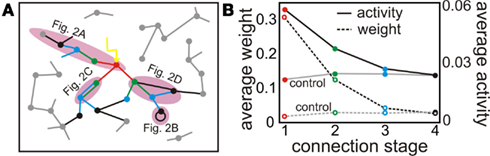
Figure 1. Given a strong external input synaptic plasticity combined with synaptic scaling (equation 1) leads to an input trace similar to a cell assembly. (A) Schematic of post-synaptic connectivity of selected neurons up to stage five. The red neuron receives a strong external input (yellow arrow). Parts of the descendent network stages are highlighted to show the general connectivity structures analyzed in this study (c.f. Figure 2). (B) Neural activities (dashed lines) and weights (solid lines) after stabilization found for the first four stages. Weights and activities of the stages linked to the external input (black) are significantly larger compared to control neurons (gray) over the first three stages representing an input trace (cell assembly).

In the current study we are going to investigate the sphere of influence of the given external input on the fixed points of weights and activities of the network dependent on the underlying connectivity. For this, we split the complex random network (c.f. Figure 1A) in smaller, more generalized parts (e.g., purple areas in Figures 1A and 2) and analyze their influence on size (number of neurons/stages) and strength (weights) of the input trace (cell assembly).

FIGURE 2

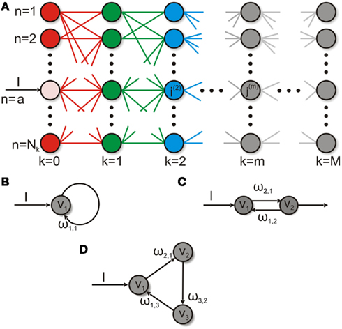
Figure 2. The different networks investigated in this study. (A) A feed-forward network consists of M layers each with N_k neurons. Each neuron j ^m of each layer m connects to all neurons of the source-layer m − 1 and target-layer m + 1 and has no connections within its layer. In this example neuron n = a of the first layer k = 0 (pink) receives an input ℑ while the other neurons within this layer do not. (B) The smallest recurrent system: a neuron with a self-connection receiving external input. (C) A neuron receives an external input and is recurrently connected to another neuron. (D) Three neurons build a ring structure.

First, we obtain analytical results for excitatory feed-forward networks (Figure 2A) with and without lateral connections and with feed-forward or lateral inhibition. In addition, we derive stability constraints for the maximally allowed input strength. An interesting result is that the combination of plasticity and scaling reduces lateral signal dispersion in feed-forward networks even without inhibition.

Second, we investigate recurrent network structures which are generally more difficult to handle and analytical results are hard to derive (here we mostly rely on numerics). However, we still provide analytical insights which lead to two observation: First, recurrences increase activity compared to feed-forward structures and, therefore, extend the input trace (cell assembly) within the network. Second, if we connect neurons so that they form a recurrent ring, the stability of rings of different size in a network is determined by the stability of the ring with the smallest number of neurons. All these aspects are consolidated by numerics.

To help navigating through this diversity, we provide at the end of most subsections a short paragraph that summarizes the results from this subsection. As part of the Discussion section we, finally, summarize all main findings (also in Table 1) and based on the main findings of this study give an example of a topology which results in localized cell assemblies (Figure 8).

TABLE 1

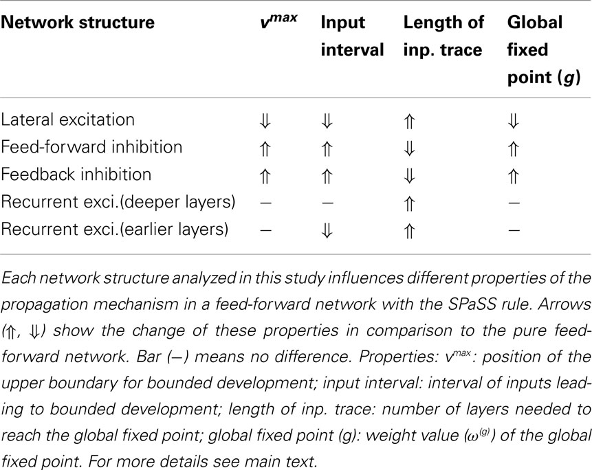
Table 1. Tabular summary of the influence of different network structures compared to a pure feed-forward network.

2. Materials and Methods

2.1. General Fixed Point Analysis

The differential equations of weights and activities for different network topologies are derived in the main text and analyzed according to their fixed point structure. This analysis is based on standard methods for a given set of differential equations $\frac{d\omega }{dt}=\stackrel{.}{\omega }=\gamma \left(\omega \right)$ determining the dynamics of ω and its fixed points ω*, where $\stackrel{.}{\omega }=0.$ To assess the stability of these fixed points, we analytically computed the Jacobian J_γ(ω) of γ; a fixed point ω* is stable if all eigenvalues at ω = ω* are smaller than zero, and unstable otherwise. Numerics are done by solving the differential equations with the Euler method.

2.2. Feed-Forward Network

The feed-forward network (see Figure 2A) consists of M layers each with N_k neurons. Each neuron n ∈ {1, …, N} of each layer k ∈ {0, …, M − 1} has an all-to-all connection to all neurons of the target-layer k + 1 and no connection to neurons within its layer k if not stated differently. Therefore, neuron n = i^(m) of layer m receives its inputs from all neurons j^(m−1) of layer m − 1 with their activities $v_j^{\left(m-1\right)}$ via synapses of strength ${\omega }_{i,j}^{\left(m\right)}.$ Thus, the output activity $v_i^{\left(m\right)}$ of neuron i^(m) is the function $F\left({\sum }_j^{N_{m-1}}{\omega }_{i,j}^{\left(m\right)}\cdot v_j^{\left(m-1\right)}\right).$ It will be transmitted to all neurons of layer m + 1. For simplicity, in this study the function F is chosen to be the identity which does not influence the results qualitatively (Tetzlaff et al., 2011).

3. Results

3.1. Feed-Forward Networks

3.1.1. Weights and activities in feed-forward networks

The simplified structure in Figure 2A depicts how an input signal to a random network is traveling along topological stages (layers) within this network and how the network “reacts” to the input by adapting weights and activities. For this we simulate the behavior of such a feed-forward network with one neuron per stage (c.f. Figures 1A and 3) given a noisy input to layer one (activity of red neuron). As shown before (Figure 1), this activity leads to a strong post-synaptic synapse resulting in high (but not as high as red) activity at layer 1 (green neuron). This behavior is propagated until the activity vanishes in layer 4 (gray). This is the basic property of the above described input trace (cell assembly). Even if the input is reduced for a certain duration the network can re-adapt to its previous stable state very fast (c.f. Figure 3). Thus, even with a noisy external input, the network can construct a stable cell assembly along several stages.

FIGURE 3

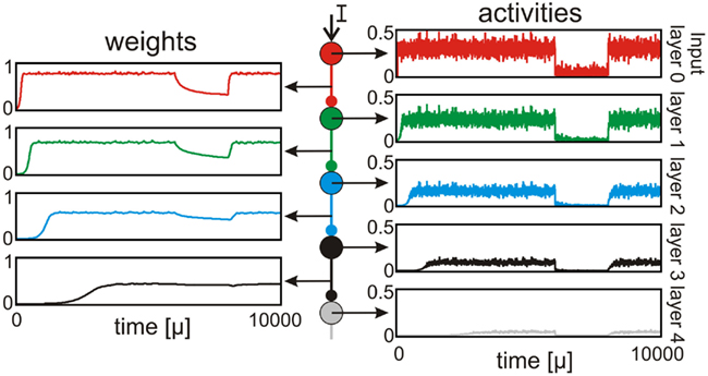
Figure 3. A noisy external input leads to propagation of activity along several stages. The first neuron (red) receives a time varying (noisy) input which leads to a strong post-synaptic synapse. Thus, the activity is transmitted to the next stage (green) resulting in high (but smaller than the input) activity and weight. This transmission occurs along several stages until the activity vanishes (gray). Even a short decrease of the input can be compensated quite fast.

In the following we analyze analytically the fixed points of weights and activities for each stage dependent on feed-forward connections and the input. We consider an input of average strength ℑ given to a neuron j⁽⁰⁾ = a of the first layer k = 0 (pink neuron in Figure 2A), which leads then to the input activity $v_{j=a}^{\left(k=0\right)}=v_a^{\left(0\right)}=\Im$ of the first layer (the other neurons in layer k = 0 have $v_{j\ne a}^{\left(0\right)}=0$). Next, we calculate the weights ${\omega }_{i,j}^{\left(1\right)}$ and activities $v_i^{\left(1\right)}$ of a neuron i⁽¹⁾ of the next layer k = 1 assuming that the dynamics have stabilized:

$v_i^{\left(1\right)}=\sum _{j=1}^N{\omega }_{i,j}^{\left(1\right)}\cdot v_j^{\left(0\right)}={\omega }_{i,a}^{\left(1\right)}\cdot v_a^{\left(0\right)}={\omega }_{i,a}^{\left(1\right)}\cdot \Im .$ (4)

Given this result, equation (1) and $u_j^{\left(m\right)}=v_j^{\left(m-1\right)}$ the dynamics for weights in the second layer write

$\begin{array}{c}{\stackrel{.}{\omega }}_{i,a}^{\left(1\right)}=\mu \left(v_a^{\left(0\right)}\cdot v_i^{\left(1\right)}+{\kappa }^{-1}\left(v_T-v_i^{\left(1\right)}\right)\cdot {\left({\omega }_{i,a}^{\left(1\right)}\right)}^2\right)\\ =\mu \left({\Im }^2\cdot {\omega }_{i,a}^{\left(1\right)}+{\kappa }^{-1}\left(v_T-\Im \cdot {\omega }_{i,a}^{\left(1\right)}\right)\cdot {\left({\omega }_{i,a}^{\left(1\right)}\right)}^2\right)\end{array}$ (5)

This equation still has only one fixed point in the excitatory regime (i.e., ω > 0):

${\omega }_{i,a}^{\left(1\right)}=\frac{v_T}{2\Im }+\sqrt{\kappa \Im +\frac{v_T^2}{4{\Im }^2}}\equiv {\omega }_{\left(\cdot \right),a}^{\left(1\right)}$ (6)

Substituting this solution into equation (4) gives

$v_i^{\left(1\right)}=\frac{v_T}{2}+\sqrt{\kappa {\Im }^3+\frac{v_T^2}{4}}\equiv v_{\left(\cdot \right)}^{\left(1\right)}$ (7)

We write $v_{\left(\cdot \right)}^{\left(m\right)}$ as this solution applies for all i⁽¹⁾∈{1, …, N₁} of layer k = 1 because neuron j⁽⁰⁾ = a is connected to all neurons of layer k = 1.

All neurons of layer k = 1 have the same activity and since we use an all-to-all connectivity between each layer, neurons within each subsequent layer k ≥ 1 will have equal activity, too. Hence, the (equal) activity of each neuron in layer k = m and also the (equal) strength of each weight projecting to layer k = m merely depends on the (equal) activity of each neuron in layer k = m − 1 and the number of neurons N_(m−1) in this layer:

$\begin{array}{l}{\omega }_{i,\left(\cdot \right)}^{\left(m\right)}=\frac{v_T}{2N_{\left(m-1\right)}{v}_{\left(\cdot \right)}^{\left(m-1\right)}}\\ +\sqrt{\kappa v_{\left(\cdot \right)}^{\left(m-1\right)}+{\left(\frac{v_T}{2N_{\left(m-1\right)}{v}_{(\cdot )}^{\left(m-1\right)}}\right)}^2}\equiv {\omega }_{\left(\cdot \right),\left(\cdot \right)}^{\left(m\right)}\text{\hspace{1em}(8)}\\ v_i^{\left(m\right)}=N_{\left(m-1\right)}\cdot {\omega }_{i,\left(\cdot \right)}^{\left(m\right)}\cdot v_{\left(\cdot \right)}^{\left(m-1\right)}=\frac{v_T}{2}\\ +\sqrt{\kappa N_{\left(m-1\right)}^2{\left(v_{(\cdot )}^{\left(m-1\right)}\right)}^3+{\left(\frac{v_T}{2}\right)}^2}\equiv v_{\left(\cdot \right)}^{\left(m\right)}\text{\hspace{1em}(9)}\end{array}$

In the next subsection we will analyze and discuss the dynamics of these equations for different parameters given the same number of neurons in each layer (N = N_k, ∀k∈{0, …, M − 1}).

3.1.2. Development of weights and activities along layers

Equations (8) and (9) describe the dynamics of weights and activities in a feed-forward network that is stimulated by just one input. When we look at the propagation of the activity (after stabilization of the weights) for different parameter values, we will find two qualitatively different scenarios: Activities will increase (divergent regime) or decrease (bounded regime) from layer to layer. As divergence should be avoided and bounded development enforced, the following relation has to be fulfilled for all neurons $m>1:v_{\left(\cdot \right)}^{\left(m\right)}\le v_{\left(\cdot \right)}^{\left(m-1\right)}.$ We now calculate lower and upper bounds for the activity and the weights so that we stay in the bounded regime.

$\begin{array}{c}\hfill v_{\left(\cdot \right)}^{\left(m\right)}\stackrel{!}{\le }{v}_{\left(\cdot \right)}^{\left(m-1\right)}\\ \hfill \frac{v_T}{2}+\sqrt{\kappa N^2{\left(v_{(\cdot )}^{\left(m-1\right)}\right)}^3+{\left(\frac{v_T}{2}\right)}^2}\le v_{\left(\cdot \right)}^{\left(m-1\right)}\\ {\left(v_{(\cdot )}^{\left(m-1\right)}\right)}^3-\frac{1}{\kappa N^2}{\left(v_{(\cdot )}^{\left(m-1\right)}\right)}^2+\frac{v_T}{\kappa N^2}{v}_{\left(\cdot \right)}^{\left(m-1\right)}\le 0\hfill \end{array}$

$\begin{array}{c}\Rightarrow v_{\left(\cdot \right)}^{\left(m-1\right)}\le 0\hfill \\ \hfill \vee \frac{1}{\kappa N^2}\left(\frac{1}{4\kappa N^2}-v_T\right)\ge {\left(v_{(\cdot )}^{\left(m-1\right)}-\frac{1}{2\kappa N^2}\right)}^2\end{array}$

The first inequality applies for negative firing rates. Thus, we ignore this result in the following. The second inequality defines an upper and lower bound on the activity or rather on the input ℑ:

$\begin{array}{rcl}{v}_{\left(\cdot \right)}^{\left(m-1\right)}& \le \frac{1}{2\kappa N^2}+\sqrt{\frac{1}{\kappa N^2}\left(\frac{1}{4\kappa N^2}-v_T\right)}\equiv v^{max}& \text{(10)}\\ v_{\left(\cdot \right)}^{\left(m-1\right)}& \ge \frac{1}{2\kappa N^2}-\sqrt{\frac{1}{\kappa N^2}\left(\frac{1}{4\kappa N^2}-v_T\right)}\equiv v^{min}& \text{(11)}\end{array}$

The two constraints equations (10) and (11), and the nullcline for the weights (equation A1 in Appendix) define the weight-activity phase space (cf. Figures 4A–C) as well as the development of the fixed points of activity and weight along layers or rather stages m (cf. Figures 4D–E) in a feed-forward network. The trajectory depends on the terminal firing rate v_T and the number of neurons N (c.f. Figure 4).

FIGURE 4

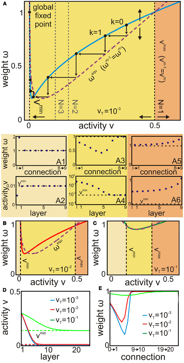
Figure 4. The phase space of a feed-forward network and how the representation of a given input depends on the parameter v_T. (A–C) The constraints v^min, v^max (vertical black dashed lines), and ω^equ (purple dashed line) define the direction of change of weight and activity (arrows) from layer to layer on the fixed point curve (colored continuous line). (A1–A6) The sub-panels show the fixed point values of the weights (top) and activities (bottom) of the layers at different regimes (colored according to the phase space). (D,E) Resulting from these curves the number of layers m needed to reach the global fixed point (thus, representing an input) varies for different v_T. Dashed lines are the respective v^min lines. For more details see main text. Parameters: k = 2, N = 1; (A) v_T = 10⁻³; (B) v_T = 10⁻²; (C) v_T = 10⁻¹(D–E) ℑ = 0.3.

The phase space consists of two qualitatively different curves. The first class of curves represents the fixed points of each layer (equation 8). These fixed points do not depend on layer number k directly but on the input to this layer which is the output of the preceding layer $v_i^{m-1}.$ In Figures 4A–C these fixed points are represented by the solid line. The second class of curves deals with the layer to layer fixed points of our system, i.e., with the previously calculated two constraints equations (10) and (11) and, additionally, equation (A1) for the weights. These constraints define the limits of a region within which activity stays bounded from layer to layer. In Figures 4A–C these curves are dashed lines (vertical black lines are v^min and v^max; the purple line is the nullcline ω^equ for ω^m = ω^m−1). The constraints v^min and v^max divide the phase space into three qualitatively different regimes: if the activity of only a single layer is smaller than v^min, the activity of the next layer “jumps” to v^min and stays there for the descendant layers. If the activity is larger than v^max, activities increases from layer to layer; only if the activity stays between v^min and v^max, activities decrease from layer to layer and stay bounded (c.f. arrows in Figure 4A). Only v^max is significantly influenced by N leading to a smaller stable range as more neurons excite one neuron in the next stage.

Now we can understand how fixed points develop from layer to layer and, thus, how large a cell assembly, given input strength ℑ, gets.

First, we apply an input from the bounded regime that causes activities and weights of the first layer to converge to their fixed points which lie on the blue line (e.g., k = 0 in Figure 4A). The resulting activity v⁽⁰⁾* is then transmitted to the next layer and causes in turn weights of the next layer to converge. Intuitively, this is visualized by a line going downward until it reaches the weight nullcline ω^equ. From here, weights together with the activity of the previous layer once again cause the activity of the next layer (k = 1) to converge, too. This is visualized by a line going leftwards to the blue fixed point curve.

This process repeats from layer to layer until the global fixed point at (v^(g) = v^min, ω^(g) = 1) is reached for layer k = g. Activities and weights will not change for subsequent layers k > g. In other words, the external input cannot influence layers k > g.

Thus, in a pure feed-forward network any kind of information storage can only exists for the first k layers since the system reaches its global fixed point for layers beyond k independent of the initial input (as long as the input is in the bounded regime).

3.1.3. Influence of parameters

To assess the capacity of information storage (size of input trace), we need to determine the influence of network parameters on g. It turns out that most influence on g is caused by v_T. Figures 4D,E demonstrate activity and weight development for three different values of v_T. Note that although the development moves along discrete layers, we plot continuous lines.

Next, we estimate the “number of jumps” from the distance between weight nullcline w^equ and the blue fixed point curve (c.f. arrows between blue and purple line in Figure 4A). A smaller distance (compare Figures 4B,C) leads to smaller “jumps” from layer to layer which in turn leads to more layers toward the global fixed point. However, at the same time the difference between v^min and v^max decreases which leads to a reduced total distance between the input value and v^min.

In Figures 4A1–A6 we also show numerical results of activity and weight development when the input is chosen to be in one of each of the three different regimes; this confirms our analytical observations. For inputs greater than v^max the network diverges (Figures 4A5 and A6). For inputs less than v^min the network converges quickly to its global fixed point (v = v_min, ω = 1; Figures 4A1 and A2). Only for inputs between v^min and v^max (Figures 4A3 and A4) we notice distinctively different fixed points along several layers until at around layer eight the global fixed point is eventually reached. Thus, such a feed-forward network with inputs between v^min and v^max stores different values for activities and weights, here up to layer 7. The numerical results of A3 and A4 are qualitatively very similar to the analytical curves in Figures 4D,E.

We now define the theoretical limits of this system. On the one hand we see from Figure 4D that in order to maximize g the distance between v^max (equation 10) and v^min (equation 11) should be small and v_T should then be ξ = (4κN²)⁻¹:

$\underset{v_T\to \xi }{lim}{v}^{max}=\underset{v_T\to \xi }{lim}{v}^{min}=\frac{1}{2\kappa N^2}$

Given an input between v^min and v^max, the system would need m → ∞ to reach v^min. However, with v_T → (4κN²)⁻¹ the interval (v^min, v^max) from which inputs can be chosen becomes smaller – eventually zero – and the network is specialized to “store” only a few (or one) distinct inputs. Additionally, the difference between input representation (minimum fixed point weight ω^min) and global fixed point (ω^(g) = 1) also becomes smaller (green curve in Figures 4D,E). So a noisy read-out of the stored inputs is complicated as an input difference could easily fall inside the noise level. On the other hand, to get a stable read-out and at the same time to “store” a large range of different inputs, the difference between v^min and v^max should be maximized. From equations (10) and (11) we find that v_T should be as negative as possible, however, in a pure feed-forward network v_T < 0 would lead to a negative firing rate for v^(g) = v^min < 0 which is mathematically possible but biologically implausible. Thus, v_T should minimally go to zero:

$\begin{array}{c}\underset{v_T\to 0}{lim}{v}^{max}=\frac{1}{\kappa N^2}\\ \underset{v_T\to 0}{lim}{v}^{min}=0.\end{array}$

To sum up, there is a trade-off, which depends on v_T, between the number of layers representing an input and the stability of this representation against noise. On the one hand, a high v_T ensures an extended representation over many layers, but, on the other hand, this representation is now quite susceptible to noise during the read-out process as fixed points are close to each other, and vice versa for a small v_T.

3.1.4. Signal dispersion in a feed-forward network with local connectivity

Signals and therefore information in feed-forward networks are transmitted from layer to layer. If we demand that there is still information of our initial signal even after many layers, the network has to maintain the spatio-temporal integrity of inputs. Ideally, inputs should not disperse randomly both in space and in time.

We therefore test the capability of a feed-forward network (Figure 2C) for signal representation and transportation. The synapses of the network are modified by the SPaSS rule. Constant weights represent the control (to mimic, for instance, weight hard-bounds). In the first of our two scenarios we present a spatially restricted signal (transport signal) to the first layer and then measure the dispersion along layers (Figures 5A,B). In the second scenario we inject as an input two adjacent signals with a small spatial gap between them (resolution signal; Figures 5C,D). With both scenarios we are able to analyze the network’s capability to differentiate its inputs after a certain number of layers. Different from the previously analyzed network the feed-forward network is constructed as follows: each neuron projects and in turn receives synapses to and from a neuron at the same position and its two neighbors in the next and the former layer.

FIGURE 5

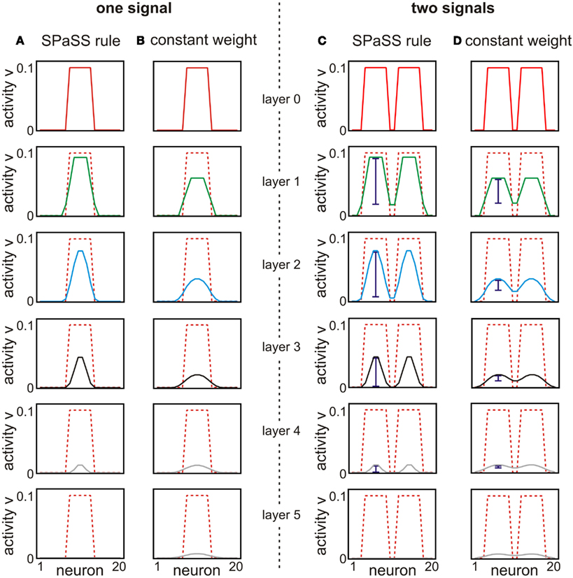
Figure 5. Signals travel along layers in a pure feed-forward network depending on the used plasticity mechanisms. (A,B) Spatial smearing of a signal is analyzed by presenting one spatially restricted input to a small group of neurons in the feed-forward network. Constant weights ω_c lead to smearing (compare activity profile of given layer in red with the footprint of the original signal shown by the dashed lines). The SPaSS rule produces much less smearing and the signal propagates along layers mostly remaining inside the originally stimulated region until it vanishes. (C,D) This focusing effect of the SPaSS rule increases the resolution to distinguish two spatially distant signals in higher (e.g., blue bars of layer 1) and deeper layers (e.g., layer 3). Parameters: ω_c = 0.2, κ = 2, v_T = 10⁻², ℑ = 0.1, ℑ_background = 10⁻⁴, N = 20, M = 10 the first six layers are shown.

If the weights are set to a constant value ω_c, the input smears out with every subsequent layer. This is best visible in Figure 5B when comparing the activity profile of each layer with the dashed lines of the original signal. Additionally, the amplitude of the signal gets reduced with every subsequent layer. Although smearing is reduced by using smaller constant weights ω_c, this also leads to a stronger reduction of amplitude. The SPaSS rule, on the other hand, can reduce (after weight stabilization) both smearing and amplitude reduction (cf. Figure 5A) at the same time. It is interesting to note that only in the first layer the activity of the border neurons is significantly increased. In all subsequent layers, the signal amplitude of these border neurons does not increase but merely follows the general reduction of signal amplitude.

In the second scenario smearing reduces the gap between the two initially separate signals from layer to layer (Figure 5D). For constant weights ω_c the signals are difficult to distinguish after the third layer (Figure 5D). For plastic synapses the resolution decreases, too, but both signals are still distinguishable until the signal vanishes at layer five (Figure 5C). This effect has its origin in the scaling mechanism which tries to balance incoming signals. This leads to a suppression of later signals while at the same time the strong forward pathways are being maintained.

In summary, the SPaSS rule avoids a spreading or rather smearing of spatially restricted signals in deep layers of feed-forward networks. Therefore, the rule ensures that spatially distinct signals presented to a network are still distinguishable after passing several neuronal layers.

3.1.5. Feed-forward networks with excitatory and inhibitory connections

In this section we consider step by step our feed-forward network with -i- lateral excitatory connections within layers (top row in Figure 6), -ii- feed-forward inhibition (middle row in Figure 6), and -iii- feedback (self-)inhibition (bottom row in Figure 6) while all intra-layer connections stay constant. Under these constraints, analytical results can still be obtained and we state only the main equations here. All calculations – similar to those shown above – are provided in the Appendix. In principle we could also do analytics for mixtures of the structures presented in Figure 6 but calculations get lengthy and opaque then, and the same is true for plastic intra-layer connections.

FIGURE 6

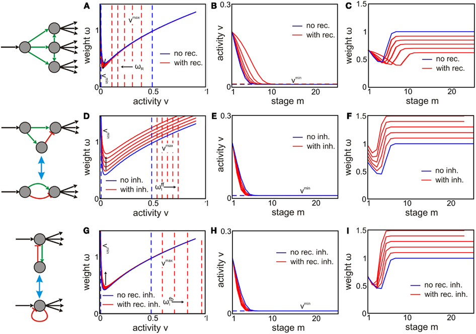
Figure 6. Inhibition and recurrent connections influence fixed points of activity and weights from layer to layer. The (A,D,G) show the phase space of the modified feed-forward networks (blue lines show the control from Figure 4A). Different structures results in different activity (B,E,H) and weight (C,F,I) development over stages m. (A–C) In the feed-forward network there are constant excitatory recurrent connections of weight ω_R within each layer. These recurrences shift the constraints v^min and v^max of the fixed points and narrow the regime of possible inputs. However, the length of a trace and its difference are larger for stronger recurrences (Rω_R). (D–F) Fixed points with feed-forward inhibition (G–I). As (A–C), however, with inhibitory recurrent connections. Inhibition (feed-forward and feedback) enlarges the regime of inputs resulting in stable development over layers. However, length and difference of the traces are shortened. Parameters: κ = 2, v_T = 10⁻², N = 1, and Rω_R/I = 0, 0.1, …, 0.5. For (B,C,E,F,H,I) ℑ = 0.2.

3.1.5.1 Lateral excitation. First we introduce lateral excitatory connections with weights ω_R (top row in Figure 6). We consider a system in which each neuron i^(m) of layer m still receives input from all neurons j^(m−1) of the previous layer m − 1 and, additionally, inputs from R neurons within its own layer m. As all neurons in a layer receive the same input, the activity $v_i^{\left(m\right)}$ is the same for all these neurons:

$\begin{array}{c}{v}_i^{\left(m\right)}=\sum _{j=1}^N{\omega }_{i,j}^{\left(m\right)}{v}_j^{\left(m-1\right)}+\sum _l^R{\omega }_R{v}_l^{\left(m\right)}\hfill \\ \hfill =N{\omega }_{\left(\cdot \right),\left(\cdot \right)}^{\left(m\right)}{v}_{\left(\cdot \right)}^{\left(m-1\right)}+R{\omega }_R{v}_{\left(\cdot \right)}^{\left(m\right)}\equiv v_{\left(\cdot \right)}^{\left(m\right)}\text{\hspace{1em}(12)}\end{array}$

If we compare fixed point solutions (equations A2 and A3 in Appendix) and constraints (equations A4–A6 in Appendix) with those of the pure feed-forward network without lateral excitatory connections (equations 8–11; equation A1 in Appendix), we find that only the number of input neurons N is rescaled by the number of lateral excitatory connections R so that we can replace

$\frac{N}{1-R{\omega }_R}=N_{Lat}\left(withR{\omega }_R<1\right).$ (13)

A larger number of lateral excitatory connections R and/or stronger weights ω_R increase the effective number N_Lat of input neurons per layer to neuron i^(m). Such an increase leads to a strong decrease in v^max while the change in v^min remains negligible (dashed lines in Figure 6A). Thus, for a stable trace the inputs are now restricted to a smaller region. The positions of fixed points within a layer (continuous red lines), however, do not change much compared to the pure feed-forward network (blue line). This finding lets us expect that global convergence is reached earlier. However, this does not apply (see Figures 6B,C) as layer to layer fixed points for ω shift (not shown), too, leading to almost the same activity value. Only the weight value of the global fixed point ω_global is reduced. This depends on the strength of the lateral excitatory connections (ω_global ≈ 1 − Rω_R; see Figure 6C, constant parts of the curves). However, more layers are needed to reach this global fixed point (Figure 6B).

Thus, with respect to signal dispersion, lateral excitation in feed-forward networks leads to a reduced decay of activity from layer to layer compared to a pure feed-forward structure (Figure 5) without effecting the smearing effect much. Thus, as smearing remains limited, distinct signals are transported over more stages when lateral excitation is present.

3.1.5.2 Inhibition. Next, we introduce inhibitory lateral connections with weights ω_I. As we define ω_I as positive, we use a minus sign in all formulas. Inhibitory weights stay constant throughout this study and the derivative of ω_I is set to zero (ω_I = const.) because plasticity mechanisms for inhibitory synapses are still highly debated (Woodin et al., 2003; Haas et al., 2006; Caporale and Dan, 2008).

We investigate feed-forward and feedback inhibition; both types are equivalent to simpler structures (middle row in Figure 6, beneath the blue arrows) that are easier to analyze.

Feed-forward inhibition: Feed-forward inhibition (Figure 6, middle row) is an important structure in neuronal networks as, for instance, the ubiquitously present lateral inhibition can be approximated by multiple feed-forward structures.

Feed-forward inhibition (Figure 6 middle, above blue arrow) consists of three neurons of which one sends signals to the other two neurons. One of these two neurons in turn inhibits the second neuron. This neuron – receiving excitatory and inhibitory inputs – is defined to be the output. We simplify this structure to two neurons (Figure 6 middle, beneath blue arrow) which is identical to the original structure if the connection from the source neuron to the inhibitory neuron is set to the identity and neuronal transfer functions are, as before, linear. In the simplified structure the source neuron directly sends signals to the output neuron through a plastic excitatory synapse ω_E and an inhibitory synapse with constant weight ${\omega }_I^{ff}.$

The activity of the output neuron is then simply the difference between both weights multiplied with the activity of the source neuron u:

$\begin{array}{c}v=u{\omega }_E-u{\omega }_I^{ff}\\ =u\left({\omega }_E-{\omega }_I^{ff}\right).\end{array}$ (14)

The results for fixed points and constraints (equations A8–A12 in Appendix) show that feed-forward inhibition increases the region of a stable input trace defined by the difference between v^max and v^min (Figure 6D). The length of the input trace (cell assembly), however, decreases (Figures 6E,F). If we compare this behavior with our pure feed-forward network, we find that feed-forward inhibition influences the dynamics similar to a change in v_T toward smaller values (Figure 4). The global stable fixed point weight, however, increases with higher inhibitory weights ω_I for feed-forward inhibition (Figure 6F, constant parts of the curves) but not when reducing v_T; then it always stays at a value of 1 (Figure 4E).

In summary, feed-forward inhibition in a feed-forward network effects the fixed point structure in a similar way as a reduced v_T in a pure feed-forward network.

Feedback inhibition: Conceptually different to feed-forward inhibition is feedback inhibition (Figure 6, bottom). Here, a neuron inhibits itself via a second neuron (Figure 6 bottom, above blue arrow). The second neuron receives excitatory input from – and in turn inhibits – the first neuron which receives inputs from preceding layers and sends signals to subsequent layers. We simplify this structure, similar to the feed-forward inhibitory structure, by setting the excitatory weight to one and, as we do anyhow by (again) using linear transfer functions for all neurons (Figure 6 bottom, beneath blue arrow). Thus, we have one neuron left which inhibits itself with constant weight ${\omega }_I^{fb};$ only the weight ω_E is plastic.

Therefore, the output activity v of the neuron is:

$\begin{array}{rcl}v& =u{\omega }_E-v{\omega }_I^{fb}& \text{(15)}\\ \iff v& =\frac{u{\omega }_E}{1+{\omega }_I^{fb}}.& \text{(16)}\end{array}$

The equations for fixed points and constraints (equations A16–A18 in Appendix) determine the phase space of such a system (Figure 6G). The influence of feedback inhibition mainly shifts v^max to higher activity values – similar to feed-forward inhibition. This again enlarges the regime of inputs that results in a stable input trace. However, such a representation needs less layers (Figure 6H) than in a pure feed-forward network.

In summary, in a feed-forward network feedback inhibition has similar effects as feed-forward inhibition but already smaller inhibitory weights ω_I yield the same results. Another difference is that the fixed point curve (equation A18 in Appendix) shifts less than for feed-forward inhibition and the dynamics of a network with feedback inhibition are more similar to the dynamics of a pure feed-forward network.

3.2. Recurrent network structures

Until now we looked only at feed-forward structures but recurrent structures are as important, for instance, to understand the dynamics of randomly connected networks. For the rest of this study we will focus on recurrent network structures. We start with presumably the simplest recurrent system: a self-connected neuron (Figure 2B) and then move on to slightly more complex ring-like structures (Figures 2C,D).

Two main results emerge from this investigation. First, the resulting activities v in different network structures after stabilization are ordered as follows: self − connected > bi − directional > three − ring > N − ring > feed − forward. Intuitively we need to consider that recurrent structures lead to a self-enhancement of activity but at the same time the number of neurons that are involved in such a recurrent ring decrease the activity if connections are on average below 1. As a consequence a second, more important observation arises: recurrent connections can be indeed stabilized by the SPaSS rule and if a recurrent structure with only a few number of neurons involved is stable, then all recurrent structures with more neurons involved will be stable, too.

3.2.1 Self-connected neurons

The simplest recurrent network is a single neuron with an input ℑ and a self-connecting synapse with weight ω (Figure 2B). The activity v_t at time t of such a neuron is simply the sum of a constant external input ℑ and the weighted output of the neuron a time step before. (Instead of one time step a fixed delay term d could be used.)

$v_t=\Im +{\omega }_t\cdot u_t=\Im +{\omega }_t\cdot v_{t-1}$ (17)

To obtain stability both variables v and ω have to be constant over time, i.e., $\stackrel{.}{\omega }$ = 0 and v_t = v_t−1. This leads to the following dependency between activity and weight:

$v=\frac{\Im }{1-\omega }.$ (18)

We insert this equation into the differential equation for weight development:

$\stackrel{.}{\omega }=\mu \left(\frac{{\Im }^2}{{\left(1-\omega \right)}^2}+{\kappa }^{-1}\left(v_T-\frac{\Im }{1-\omega }\right)\cdot {\omega }^2\right)=0$ (19)

and the solutions of equation (19) are

$\begin{array}{l}{\omega }^{{*}_1}=\frac{1}{12}\left(-\sqrt{3}\gamma -\Lambda -3b\right)\\ {\omega }^{{*}_2}=\frac{1}{12}\left(-\sqrt{3}\gamma +\Lambda -3b\right)\\ {\omega }^{{*}_3}=\frac{1}{12}\left(\sqrt{3}\gamma -\Lambda -3b\right)\\ {\omega }^{{*}_4}=\frac{1}{12}\left(\sqrt{3}\gamma +\Lambda -3b\right)\end{array}$ (20)

with

$\begin{array}{l}\gamma =\sqrt{3b^2+8ac+2^{\frac{5}{2}}a\left(c^2+12ad\right){\Gamma }^{-1}+2^{\frac{4}{3}}a\Gamma },\\ \Lambda =\sqrt{6}\sqrt{\begin{array}{c}3b^2+8ac-2^{\frac{4}{3}}a\left(c^2+12ad\right){\Gamma }^{-1}-2^{\frac{2}{3}}a\Gamma \hfill \\ +3^{\frac{3}{2}}\left(b^3+4abc\right){\gamma }^{-1}\hfill \end{array}},\\ \Gamma =\left(-2c^3+27b^{2}d+72acd\right.\\ {\left.+\sqrt{-4{\left(c^2+12ad\right)}^3+{\left(-2c^3+27b^{2}d+72acd\right)}^2}\right)}^{1∕3},\\ a=v_T,b=\Im -2v_T,c=\Im -v_T,\text{and}d=\kappa {\Im }^2.\end{array}$

These solutions have to be real (complex part equals zero) and the derivative of equation (19) at these solutions has to be smaller than zero in order to stabilize the dynamics, so parameters ℑ, κ, and v_T have to be restricted. The calculations for assessing these parameters are complex and closed-forms can not be derived anymore. Therefore, the stability for a given set of parameters has to be assessed by numerical calculations of the roots. To reduce the number of parameters only the ratio of the rates (e.g., equations 8–22) κ = μ/γ is considered and we plot the maximally allowed input ℑ^max that still leads to a stable weight. All smaller inputs (0 < ℑ < ℑ^max) lead to a stable weight ω, too, and inputs above this value (ℑ > ℑ^max) lead to divergent weight dynamics. Thus, we show the parameters which lead to stable dynamics in a κ-v_T-plot with ℑ^max color coded (Figure 7A). The self-connected neuron stabilizes best if γ is as large as μ (κ ≈ 1) but for the more realistic ratios of one order of magnitude difference (κ ≈ 10) stabilization is still possible for a wide regime. Furthermore, stability requires that v_T is small or even negative. Here we stress that (1) negative v_T does not imply negative neuronal firing rates as these systems balance plasticity and scaling ($v_i^{*}\ne v_T;$ see equation 3 and Tetzlaff et al., 2011) and (2) negative v_T values can be avoided by simply adding inhibition to any of these recurrent networks (Figures 2B–D). As shown above, constant weight inhibition (Figures 6D–I) leads to a shift of the network properties toward larger allowed positive values. The general disk-like shape of the stability plot, however, does not change with inhibition added and we will thus continue to consider only excitatory recurrent networks (although v_T might be negative).

FIGURE 7

Figure 7. Different recurrent structures are stabilized by SPaSS rule. For different parameter values κ and v_T the maximal input ℑ^max leading to stable weights is calculated and shown in color code (note the different scale bars). (A) Self-connected neurons, (B) bi-directional structures, and (C) three-neuron rings are analyzed. If one structure is stabilized for a given parameter set (κ, v_T) all other structures are stable, too. Only the maximal input decreases with more direct (less neurons) recurrences.

We have confirmed our numerical calculations with simulations up to four places after the decimal point for weight ω and activity v. (For example, for κ = 2, ℑ = 0.065, and v_T = 0.01 the weight and the activity in the simulation as well as in the numerics is ω = 0.5674 and v = 0.1503 respectively).

We now compare the activity of a neuron with a self-connection v_sc with the activity v_ff of a neuron in a feed-forward structure receiving the same input ℑ if equation (19) is simplified in the following way (see also Appendix): as ω is smaller than one, weight-dependent terms of order three (Θ(ω³)) and higher can be ignored. This leads to following neuronal activity:

$v\approx \frac{\Im }{1-\sqrt{\kappa {\Im }^2\Im -v_T}}$ (21)

which is larger than v_ff = ℑ.

In summary, self-connected structures in a neuronal network will raise the risk of instability. As this instability depends on the input (or rather the activity given to the self-connected neuron) this risk will decrease if a self-connected structure is in deeper layers (because activity has already declined there). However, as the resulting fixed point activity of self-connected neurons is larger than the activity of a neuron in a feed-forward structure, self-connections will extend input trace into deeper layers.

3.2.2 Simple recurrent ring networks: bi-directional and three-ring

In recurrent networks there are also other types of recurrent structures than simple self-connected neurons. Thus, in the following we derive the influence of larger recurrences on the stability and activity of neuronal networks. Equations (A19) and (A20) in Appendix show that also for the bi-directional connection the activity is increased compared to the feed-forward networks. This effect could be expected as already constant recurrences enhance network activity, but the SPaSS rule sustains the enhancement and still guarantees stable weights. Interestingly, this effect does not depend on the position of the bi-directional structure within the feed-forward network. The second neuron can be part of the feed-forward network but it can also be outside of the layered structure.

Additionally, we numerically calculated the stable regime for different parameter values and plot the results similar to the self-connected neuron. This analysis (Figure 7B) confirms the result that stability is independent of the chosen parameters v_T and κ. However, we observe that the maximally allowed input ℑ^max that still leads to convergence increases compared to the self-connected neuron (mind the changed color scale bars in Figures 7A,B).

For the three-neuron ring an enhancement of these observations is observed. Its equations (equation A23 in Appendix) again show that for the three-ring the activity is increased, but less, as compared to the feed-forward networks.

Furthermore, we find that the stability range for the three-ring (Figure 7C) looks similar to the one discussed above (Figures 7A,B) and the maximally allowed input ℑ^max has further increased.

These considerations can be generalized in a straight-forward way for an N-ring, too (not shown).

To conclude, the results presented above confirm what we stated at the beginning of this section. First, if the smallest existing ring structure in a randomly wired recurrent network is stable, then every longer ring will be stable, too. Second, there is an ordering of the resulting activities (see Appendix):

$\begin{array}{l}\text{w}.\text{l}.\text{o}.\text{g}.v_T\to 0\\ v_{sc}\approx \frac{\Im }{1-\sqrt{\kappa \Im }}>v_{bi}\approx \frac{\Im }{1-{\omega }_{1,2}\sqrt{\kappa \Im }}>\\ v_{nr}\approx \frac{\Im }{1-{\omega }_{1,N}{\Pi }_{i=3}^N{\omega }_{i,i-1}\cdot \sqrt{\kappa \Im }}>v_{ff}=\Im ,\\ \text{with}{\omega }_{i,j}<1\forall i,j\in N\end{array}$

(self − connected > bi − directional > N − ring > feed − forward). Furthermore (similar to the direct self-connection discussed above) if one neuron connects recurrently via a ring to itself, its fixed point activity is enlarged. Thus, given a feed-forward network, this fact ensures that also all following (down stream) layers will have an increased activity and, therefore, more layers are needed to reach the global fixed point. This effect is in general even stronger with the SPaSS rule than with constant weights (c.f. section 5) as the denominator of the activity depends on the input ℑ. Thus, the length of the input trace is increased with any excitatory recurrent structure.

4. Discussion

Hebb (1949) proposed that a group of interlinked neurons forms a “cell assembly.” In this study we show that the combination of synaptic scaling and hebbian plasticity can lead to such “cell assemblies.”

Synaptic scaling is a slow biological process which interacts with faster conventional synaptic plasticity (Abbott and Nelson, 2000; Turrigiano and Nelson, 2000). In a previous study (Tetzlaff et al., 2011) we showed that the (mathematical) combination of both processes leads to stable and reasonable weight growth. In the current study we have extended the analysis of this combined plasticity and scaling (SPaSS) rule to different types of feed-forward and recurrent networks. Our main goal was to try to understand why such networks are capable of forming an input trace in a stable way, with stably enhanced weights along several network stages as shown in Figure 2B. Thus, such networks are to some degree capable of learning and storing a “cell assembly” (Hebb, 1949) along the network layers.

Our main results are: (1) feed-forward networks indeed obtain a stable sequence of fixed points along several network stages, which can still be analytically calculated. This happens for a certain input range v^min < ℑ < v^max. If the network has many layers eventually a final stable fixed point is reached for all layers k > g, after which no more useful information processing takes place. Lateral connections and inhibition (feed-forward and feedback) can modify this range of information processing, hence, the extend of the input trace (see Table 1). For the lower layers one finds that networks with a SPaSS rule reduce signal dispersion as compared to networks with constant connections (see Figure 5). (2) As soon as one introduces recurrent connections, calculations become more difficult and most results have to rely on a numerical analysis. Here we find that small excitatory recurrent structures (self-connection, or small rings) are more “dangerous” than large rings as it is easier to get unstable dynamics from small as compared to large rings. Thus, if one stabilizes the smallest ring in a network, one will find that larger rings are stable, too. However, as the resulting activity from a ring is larger than in a feed-forward structure, recurrences enhance the length of an input trace and, thus, extend the influence of an external input into the deeper layers of the network. This way a larger cell assembly representing this input is formed.

Furthermore, we can take the results obtained in this study and conclude how big a cell assembly representing an external input would be and how to change its size by parameters and connectivity. For instance, a feed-forward network with one neuron per layer (also named transmission line) and recurrent (here constant) connections between layers (comparable to section 5 and 2) would lead to an input trace with stronger weights compared to a pure feed-forward network. If we introduce additionally long-range feed-forward inhibition the input trace can be “cut” after a few stages. Thus, short-range excitatory feedback together with long-range feed-forward inhibition lead to localized cell assemblies “around” the input neuron (compare black curve in Figure 8 with gray).

FIGURE 8

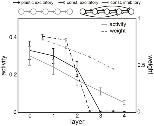
Figure 8. Connectivity shapes the size of input traces. In a pure feed-forward network (gray) an input leads to an input trace along several stages. The weights (dashed) and activities (solid) decrease from layer to layer (as already explained in section 2). On the one hand, by introducing recurrences the weights have significantly larger fixed points (see black line of the first layers), thus, the cell assembly is more stable against perturbation and more prominent in the network. Long-range inhibition, on the other hand, decreases activities and weights in a way that the cell assembly is “cut” from layer to the next (here, for instance, between 2 and 3). This an example of using the results of this study to define a connectivity which leads to strongly localized cell assemblies. Parameters: ${\omega }_R={\omega }_I^{ff}=0.1;$ others see Figure 3.

Thus, the SPaSS rule naturally leads to spatially restricted formation of input representations. Such a representation might be indicative of a memory process, which is here reflected by the still very simple process of storing an input trace and this way forming a cell assembly. So far it has proven to be difficult to achieve stable representations of spatial-temporal patterns in time-continuous systems (c.f. Morrison et al., 2007 for STDP). In this study we analyzed mainly the spatial dispersion of such an input representation and how this dispersion is influenced by different connectivities. After stabilization removal of the input leads to slow forgetting, which however can be reversed quite fast by presenting the input again (see Figure 3). This process of forgetting and re-learning and, furthermore, the temporal aspect of the input representations has to be analyzed in future studies. However, the analysis here suggests that the combination of synaptic plasticity and synaptic scaling might be a good candidate to allow the formation of short term memories (Dudai, 2004) also in larger networks. The aspect of stable learning in attractor neural networks remains largely unresolved (Mongillo et al., 2008; Cutsuridis and Wennekers, 2009; Lansner, 2009) and we would hope that the results presented here will lead onward helping to solve this problem and leading to a better understanding of (short term) memory formation processes.

Conflict of Interest Statement

The authors declare that the research was conducted in the absence of any commercial or financial relationships that could be construed as a potential conflict of interest.

Acknowledgments

The research leading to these results has received funding from the European Community’s Seventh Framework Program FP7/2007-2013 (Specific Program Cooperation, Theme 3, Information and Communication Technologies) under grant agreement no. 270273, Xperience (Florentin Wörgötter), by the Federal Ministry of Education and Research (BMBF) by grants to the Bernstein Center for Computational Neuroscience (BCCN) – Göttingen, grant number 01GQ1005A, projects D1 and D2 (Florentin Wörgötter) and 01GQ1005B, project B3 (Marc Timme), by the Max Planck Research School for Physics of Biological and Complex Systems (Christian Tetzlaff).

References

Abbott, L. F., and Nelson, S. B. (2000). Synaptic plasticity: taming the beast. Nat. Neurosci. 3(Suppl.), 1178–1183.

Pubmed Abstract | Pubmed Full Text | CrossRef Full Text

Bi, G. Q., and Poo, M. M. (1998). Synaptic modifications in cultured hippocampal neurons: dependence on spike timing, synaptic strength, and postsynaptic cell type. J. Neurosci. 18, 10464–10472.

Pubmed Abstract | Pubmed Full Text

Bienenstock, E. L., Cooper, L. N., and Munro, P. W. (1982). Theory for the development of neuron selectivity: orientation specificity and binocular interaction in visual cortex. J. Neurosci. 2, 32–48.

Pubmed Abstract | Pubmed Full Text

Caporale, N., and Dan, Y. (2008). Spike timing-dependent plasticity: a hebbian learning rule. Annu. Rev. Neurosci. 31, 25–46.

Pubmed Abstract | Pubmed Full Text | CrossRef Full Text

Cutsuridis, V., and Wennekers, T. (2009). Hippocampus, microcircuits and associative memory. Neural Netw. 22, 1120–1128.

Pubmed Abstract | Pubmed Full Text | CrossRef Full Text

Dudai, Y. (2004). The neurobiology of consolidation, or, how stable is the engram? Annu. Rev. Psychol. 55, 51–86.

Pubmed Abstract | Pubmed Full Text | CrossRef Full Text

Gerstner, W., and Kistler, W. M. (2002). Mathematical formulations of Hebbian learning. Biol. Cybern. 87, 404–415.

Pubmed Abstract | Pubmed Full Text | CrossRef Full Text

Haas, J., Nowotny, T., and Abarbenel, H. D. I. (2006). Spike-timing-dependent plasticity of inhibitory synapses in the entorhinal cortex. J. Neurophysiol. 96, 3305–3313.

Pubmed Abstract | Pubmed Full Text | CrossRef Full Text

Hahnloser, R., Kozhevnikov, A., and Fee, M. (2002). An ultra-sparse code underlies the generation fo neural sequences in a songbird. Nature 419, 65–70.

Pubmed Abstract | Pubmed Full Text | CrossRef Full Text

Harris, K., Csiscvari, J., Hirase, H., Dragoi, G., and Buzsaki, G. (2003). Organization of cell assemblies in the hippocampus. Nature 424, 552–556.

Pubmed Abstract | Pubmed Full Text | CrossRef Full Text

Hebb, D. O. (1949). The Organization of Behaviour. New York: Wiley.

Lansner, A. (2009). Associative memory models: from the cell-assembly theory to biophysically detailed cortex simulations. Trends Neurosci. 32, 178–186.

Pubmed Abstract | Pubmed Full Text | CrossRef Full Text

Miller, K. D., and MacKay, D. J. C. (1994). The role of constraints in Hebbian learning. Neural Comput. 6, 100–126.

CrossRef Full Text

Mongillo, G., Barak, O., and Tsodyks, M. (2008). Synaptic theory of working memory. Science 319, 1543–1546.

Pubmed Abstract | Pubmed Full Text | CrossRef Full Text

Morrison, A., Aertsen, A., and Diesmann, M. (2007). Spike-timing-dependent plasticity in balanced random networks. Neural Comput. 19, 1437–1467.

Pubmed Abstract | Pubmed Full Text | CrossRef Full Text

Oja, E. (1982). A simplified neuron model as a principal component analyzer. J. Math. Biol. 15, 267–273.

Pubmed Abstract | Pubmed Full Text | CrossRef Full Text

Tetzlaff, C., Kolodziejski, C., Timme, M., and Wörgötter, F. (2011). Synaptic scaling in combination with many generic plasticity mechanisms stabilizes circuit connectivity. Front Comput. Neurosci. 5:47. doi:10.3389/fncom.2011.00047

CrossRef Full Text

Turrigiano, G. G., Leslie, K. R., Desai, N. S., Rutherford, L. C., and Nelson, S. B. (1998). Activity-dependent scaling of quantal amplitude in neocortical neurons. Nature 391, 892–896.

Pubmed Abstract | Pubmed Full Text | CrossRef Full Text

Turrigiano, G. G., and Nelson, S. B. (2000). Hebb and homeostasis in neuronal plasticity. Curr. Opin. Neurobiol. 10, 258–364.

CrossRef Full Text

Turrigiano, G. G., and Nelson, S. B. (2004). Homeostatic plasticity in the developing nervous system. Nat. Rev. Neurosci. 5, 97–107.

Pubmed Abstract | Pubmed Full Text | CrossRef Full Text

Woodin, M., Ganguly, K., and Poo, M. M. (2003). Coincident pre- and postsynaptic activity modifies GABAergic synapses by postsynaptic changes in Cl⁻ transporter activity. Neuron 39, 807–820.

Pubmed Abstract | Pubmed Full Text | CrossRef Full Text

Appendix

Nullcline of Weight Development Over Stages in Feed-Forward Networks:

$\begin{array}{l}{\omega }_{\left(\cdot \right),\left(\cdot \right)}^{\left(m\right)}\stackrel{!}{=}{\omega }_{\left(\cdot \right),\left(\cdot \right)}^{\left(m+1\right)}\\ {\omega }_{\left(\cdot \right),\left(\cdot \right)}^{\left(m\right)}=\frac{v_T}{2N{v}_{\left(\cdot \right)}^{\left(m\right)}}+\sqrt{\kappa v_{\left(\cdot \right)}^{\left(m\right)}+{\left(\frac{v_T}{2N{v}_{(\cdot )}^{\left(m\right)}}\right)}^2}\\ {\omega }_{\left(\cdot \right),\left(\cdot \right)}^{\left(m\right)}=\frac{v_T}{2N{v}_{\left(\cdot \right)}^{\left(m-1\right)}\cdot {\omega }_{\left(\cdot \right),\left(\cdot \right)}^{\left(m\right)}}+\sqrt{\kappa v_{\left(\cdot \right)}^{\left(m-1\right)}\cdot {\omega }_{\left(\cdot \right),\left(\cdot \right)}^{\left(m\right)}+{\left(\frac{v_T}{2N{v}_{(\cdot )}^{\left(m-1\right)}\cdot {\omega }_{(\cdot ),(\cdot )}^{\left(m\right)}}\right)}^2}\end{array}$

which simplifies to the following nullcline for weights ${\omega }_{\left(\cdot \right),\left(\cdot \right)}^{\left(m\right)}:$

${\omega }_{\left(\cdot \right),\left(\cdot \right)}^{\left(m\right)}=\frac{\kappa N}{2}{v}_{\left(\cdot \right)}^{\left(m-1\right)}+\sqrt{\frac{v_T}{N^2{v}_{\left(\cdot \right)}^{\left(m-1\right)}}+{\left(\frac{\kappa N}{2}{v}_{(\cdot )}^{\left(m-1\right)}\right)}^2}\equiv {\omega }^{\text{equ}}$ (A1)

Lateral Excitation in Feed-forward Networks

As defined in the main text, the activity of neuron i^(m) is

$v_i^{(m)}={\displaystyle \sum _{j=1}^N{\omega }_{i,j}^{(m)}}{v}_j^{(m-1)}+{\displaystyle \sum _l^R{\omega }_R}{v}_l^{(m)}=N{\omega }_{(\cdot ),(\cdot )}^{(m)}{v}_{(\cdot )}^{(m-1)}+R{\omega }_R{v}_{(\cdot )}^{(m)}\equiv v_{(\cdot )}^{(m)}$

leading to the stability assumption

$v_{\left(\cdot \right)}^{\left(m\right)}=\frac{N}{1-R{\omega }_R}{v}_{\left(\cdot \right)}^{\left(m-1\right)}{\omega }_{\left(\cdot \right),\left(\cdot \right)}^{\left(m\right)}.$

Thus, the differential equation of the weight becomes:

${\stackrel{.}{\omega }}_{\left(\cdot \right),\left(\cdot \right)}^{\left(m\right)}=\mu \left(\frac{{\left(v_{(\cdot )}^{\left(m-1\right)}\right)}^2}{1-R{\omega }_R}{\omega }_{\left(\cdot \right),\left(\cdot \right)}^{\left(m\right)}+{\kappa }^{-1}\left(v_T-\frac{v_{\left(\cdot \right)}^{\left(m-1\right)}}{1-R{\omega }_R}{\omega }_{\left(\cdot \right),\left(\cdot \right)}^{\left(m\right)}\right)\cdot {\left({\omega }_{\left(\cdot \right),\left(\cdot \right)}^{\left(m\right)}\right)}^2\right)\stackrel{!}{=}0.$

The resulting positive stable weight is

${\omega }_{\left(\cdot \right),\left(\cdot \right)}^{\left(m\right)}=\frac{v_T}{2N{v}_{\left(\cdot \right)}^{\left(m-1\right)}}\left(1-R{\omega }_R\right)+\sqrt{\kappa {\nu }_{(\cdot )}^{(m-1)}+{\left(\frac{{\nu }_T}{2N{\nu }_{(\cdot )}^{(m-1)}}(1-R{\omega }_R)\right)}^2}$ (A2)

with associated activity

$v_{\left(\cdot \right)}^{\left(m\right)}=\frac{v_T}{2}+\sqrt{\frac{\kappa N^2}{{\left(1-R{\omega }_R\right)}^2}{\left(v_{(\cdot )}^{\left(m-1\right)}\right)}^3+{\left(\frac{v_T}{2}\right)}^2}.$ (A3)

However, to guarantee bounded development for activities $\left(v_{\left(\cdot \right)}^{k=m-1}\ge v_{\left(\cdot \right)}^{k=m}\right)$ of the network two constraints, comparable to the pure feed-forward network (equations 10 and 11), have to be maintained

$\begin{array}{rcl}{v}_{\left(\cdot \right)}^{\left(m-1\right)}& \le \frac{{\left(1-R{\omega }_R\right)}^2}{2\kappa N^2}+\sqrt{\frac{{\left(1-R{\omega }_R\right)}^2}{\kappa N^2}\left(\frac{{\left(1-R{\omega }_R\right)}^2}{4\kappa N^2}-v_T\right)}\equiv v_{rec}^{max}& \text{(A4)}\\ v_{\left(\cdot \right)}^{\left(m-1\right)}& \ge \frac{{\left(1-R{\omega }_R\right)}^2}{2\kappa N^2}-\sqrt{\frac{{\left(1-R{\omega }_R\right)}^2}{\kappa N^2}\left(\frac{{\left(1-R{\omega }_R\right)}^2}{4\kappa N^2}-v_T\right)}\equiv v_{rec}^{min}.& \text{(A5)}\end{array}$

Furthermore, the ω-nullcline is:

${\omega }_{(\cdot ),(\cdot )}^{(m)}=\frac{\kappa {\nu }_{(\cdot )}^{(m-1)}}{2}\frac{N}{1-R{\omega }_R}+\sqrt{\frac{{\nu }_T}{N^2{\nu }_{(\cdot )}^{(m-1)}}{(1-R{\omega }_R)}^2+{\left(\frac{\kappa {\nu }_{(\cdot )}^{(m-1)})}{2}\frac{N}{1-R{\omega }_R}\right)}^2\equiv {\omega }_{rec}^{equ}.}$ (A6)

Feed-forward Inhibition in Feed-forward Network

Here, the activity of the output neuron is the difference between both weights multiplied with the activity of the source neuron u:

$\begin{array}{c}v=u{\omega }_E-u{\omega }_I\\ =u\left({\omega }_E-{\omega }_I\right).\end{array}$ (A7)

As mentioned in the main text, only the excitatory weight has a non-zero derivative

${\stackrel{.}{\omega }}_E=\mu \left(u^2\left({\omega }_E-{\omega }_I\right)+{\kappa }^{-1}\left(v_T-u\left({\omega }_E-{\omega }_I\right)\right)\cdot {\omega }_E^2\right).$

This equation has only a positive stable fixed point at

${\omega }_E=\frac{v_T+u{\omega }_I}{2u}+\sqrt{\kappa u+{\left(\frac{v_T+u{\omega }_I}{2u}\right)}^2-\kappa u\frac{{\omega }_I}{{\omega }_E}}.$

The term $\frac{{\omega }_I}{{\omega }_E}$ is approximately zero as ω_I is defined to be smaller than ω_E:

${\omega }_E=\frac{v_T+u{\omega }_I}{2u}+\sqrt{\kappa u+{\left(\frac{v_T+u{\omega }_I}{2u}\right)}^2}.$ (A8)

This leads to an output activity of

$v=\frac{v_T-u{\omega }_I}{2}+\sqrt{\kappa u^3+{\left(\frac{v_T+u{\omega }_I}{2}\right)}^2}$ (A9)

Also for this system there exists constraints defining if the output v is smaller than the input u:

$\begin{array}{rcl}u& \le \frac{1+{\omega }_I}{2\kappa }+\sqrt{\frac{1+{\omega }_I}{\kappa }\left(\frac{1+{\omega }_I}{4\kappa }-v_T\right)}\equiv v_{ffi}^{max}& \text{(A10)}\\ u& \ge \frac{1+{\omega }_I}{2\kappa }-\sqrt{\frac{1+{\omega }_I}{\kappa }\left(\frac{1+{\omega }_I}{4\kappa }-v_T\right)}\equiv v_{ffi}^{min}.& \text{(A11)}\end{array}$

Additionally, nullclines can be calculated for weights if the system consists of feed-forward inhibition motifs linked together in a feed-forward structure:

${\omega }_E=\frac{\kappa u}{2}+{\omega }_I+\sqrt{\frac{v_T}{u}+{\left(\frac{\kappa u}{2}\right)}^2-\kappa u{\omega }_I}\equiv {\omega }_{ffi}^{equ}.$ (A12)

Feedback inhibition

The output activity v of the neuron is

$\begin{array}{l}v=u{\omega }_E-v{\omega }_I\\ \iff v=\frac{u{\omega }_E}{1+{\omega }_I}\end{array}$ (A13)

and, thus, the dynamics of the excitatory weight is

${\stackrel{.}{\omega }}_E=\mu \left(\frac{u^2{\omega }_E}{1+{\omega }_I}+\frac{1}{\kappa }\left(v_T-\frac{u{\omega }_E}{1+{\omega }_I}\right)\cdot {\omega }_E^2\right).$ (A14)

The positive stable fixed point of this equation is

${\omega }_E=\frac{v_T}{2u}\left(1+{\omega }_I\right)+\sqrt{\kappa u+\frac{v_T^2}{4u^2}{\left(1+{\omega }_I\right)}^2}$ (A15)

and the related output activity of this structure is

$v=\frac{v_T}{2}+\sqrt{\kappa \frac{u^3}{{\left(1+{\omega }_I\right)}^2}+\frac{v_T^2}{4}}.$ (A16)

The constraints of this system for having a smaller output v than input u are

$\begin{array}{rc}u\le \frac{{\left(1+{\omega }_I\right)}^2}{2\kappa }+\sqrt{\frac{{\left(1+{\omega }_I\right)}^2}{\kappa }\left(\frac{{\left(1+{\omega }_I\right)}^2}{4\kappa }-v_T\right)}\equiv v_{fbi}^{max}& \text{(A17)}\\ u\ge \frac{{\left(1+{\omega }_I\right)}^2}{2\kappa }-\sqrt{\frac{{\left(1+{\omega }_I\right)}^2}{\kappa }\left(\frac{{\left(1+{\omega }_I\right)}^2}{4\kappa }-v_T\right)}\equiv v_{fbi}^{min}.& \text{(A18)}\end{array}$

Additionally, for the weight the nullcline is

${\omega }_E=\frac{\kappa u}{2\left(1+{\omega }_I\right)}+\sqrt{\frac{v_T}{u}{\left(1+{\omega }_I\right)}^2+{\left(\frac{\kappa u}{2\left(1+{\omega }_I\right)}\right)}^2}\equiv {\omega }_{fbi}^{equ}.$ (A19)

Calculations for Bi-directional and N-ring recurrences

A bi-directional system can be written as

$\begin{array}{l}{\stackrel{.}{\omega }}_{1,2}=\mu \left(v_1{v}_2+{\kappa }^{-1}\left(v_T-v_1\right)\cdot {\omega }_{1,2}^2\right)\\ {\stackrel{.}{\omega }}_{2,1}=\mu \left(v_1{v}_2+{\kappa }^{-1}\left(v_T-v_2\right)\cdot {\omega }_{2,1}^2\right)\\ v_1=\Im +{\omega }_{1,2}\cdot v_2\\ v_2={\omega }_{2,1}\cdot v_1.\end{array}$

For the stability conditions, v₂ is inserted into v₁ and v₁ into v₂ resulting in

$\begin{array}{rc}{v}_1=\frac{\Im }{1-{\omega }_{1,2}\cdot {\omega }_{2,1}}& \text{(A20)}\\ v_2=\frac{{\omega }_{2,1}\cdot \Im }{1-{\omega }_{1,2}\cdot {\omega }_{2,1}}.& \text{(A21)}\end{array}$

This leads to the following weight equations

$\begin{array}{c}{\stackrel{.}{\omega }}_{1,2}=\mu \left(\frac{{\Im }^2\cdot {\omega }_{2,1}}{{\left(1-{\omega }_{1,2}\cdot {\omega }_{2,1}\right)}^2}+{\kappa }^{-1}\left(v_T-\frac{\Im }{1-{\omega }_{1,2}\cdot {\omega }_{2,1}}\right)\cdot {\omega }_{1,2}^2\right)\stackrel{!}{=}0\\ {\stackrel{.}{\omega }}_{2,1}=\mu \left(\frac{{\Im }^2\cdot {\omega }_{2,1}}{{\left(1-{\omega }_{1,2}\cdot {\omega }_{2,1}\right)}^2}+{\kappa }^{-1}\left(v_T-\frac{\Im \cdot {\omega }_{2,1}}{1-{\omega }_{1,2}\cdot {\omega }_{2,1}}\right)\cdot {\omega }_{2,1}^2\right)\stackrel{!}{=}0.\end{array}$

Although these equations can be solved, the solutions are complex expressions for ω_1,2 and ω_2,1 which are hard to interpret. However, the activity v1 of neuron 1 is larger than in a feed-forward network with the same input. On the other hand, given parameters μ = 0.01, γ = 0.005, ℑ = 0.065, and v_T = 0.01 the activity v₁ = 0.0746 > ℑ is still smaller than for the self-connected neuron (v = 0.1503). The activity of neuron 2 for these parameters is also larger than the activity of the second neuron in the feed-forward network (v₂ = 0.0343 > 0.0290 = v^k=1). This can also be shown by an approximation of ${\stackrel{.}{\omega }}_{2,1}=0,$ thereby neglecting all terms of order $\theta \left({\omega }_i^3\right)$ and higher as they are small (ω_i < 1) anyhow:

$\begin{array}{r}\frac{\kappa {\Im }^2\cdot {\omega }_{2,1}}{{\left(1-{\omega }_{1,2}\cdot {\omega }_{2,1}\right)}^2}+\left(v_T-\frac{\Im \cdot {\omega }_{2,1}}{1-{\omega }_{1,2}\cdot {\omega }_{2,1}}\right)\cdot {\omega }_{2,1}^2=0\\ \iff \left(v_T{\omega }_{1,2}+\Im \right)\cdot {\omega }_{1,2}\cdot {\omega }_{2,1}^3-\left(2v_T{\omega }_{1,2}+\Im \right)\cdot {\omega }_{2,1}^2+v_T{\omega }_{2,1}+\kappa {\Im }^2=0\\ \text{without}\theta \left({\omega }_i^3\right)\Rightarrow -\Im {\omega }_{2,1}^2+v_T{\omega }_{2,1}+\kappa {\Im }^2=0.\end{array}$

The only stable weight from this approximation that is positive is equal to the feed-forward weight ωff (equation 1) with input ℑ and N = 1 (equation 8). Thus, the activity v₂ of neuron 2 is approximately

$v_2=\frac{{\omega }_{2,1}\cdot \Im }{1-{\omega }_{1,2}\cdot {\omega }_{2,1}}\approx \frac{{\omega }^{ff}\cdot \Im }{1-{\omega }_{1,2}\cdot {\omega }^{ff}}=\frac{v^{k=1}}{1-{\omega }_{1,2}\cdot {\omega }^{ff}}>v^{k=1},\text{as}{\omega }_{1,2},{\omega }^{ff}<1.$ (A22)

Furthermore, the activity of the first neuron receiving external input is approximately

$v_1=v_{bi}=\frac{\Im }{1-{\omega }_{1,2}{\omega }_{2,1}}\approx \frac{1}{1-{\omega }_{1,2}{\omega }^{ff}}.$ (A23)

Therefore, bi-directional connections increase the activity compared to feed-forward networks. As stated in the main text, this fact does not depend on the position of the bi-directional structure within the feed-forward network. The second neuron can be part of the feed-forward network, but it can also be outside of the layered structure.

For an N-ring with N neurons the stability conditions for the activities are

$\begin{array}{l}{v}_1^N=\frac{\Im }{1-{\omega }_{1,N}{\Pi }_{i=2}^N{\omega }_{i,i-1}}\\ v_2^N=\frac{{\omega }_{2,1}\Im }{1-{\omega }_{1,N}{\Pi }_{i=2}^N{\omega }_{i,i-1}}\\ ...\\ v_N^N=\frac{{\Pi }_{i=2}^N{\omega }_{i,i-1}\Im }{1-{\omega }_{1,N}{\Pi }_{i=2}^N{\omega }_{i,i-1}}.\end{array}$

The weight ω_2,1 can be again approximated by ω^ff if weight-dependencies of order three or even higher are neglected. Thus, the activity of neuron 1 is approximately

$v_1^N=v_{nr}\approx \frac{\Im }{1-{\omega }_{1,N}{\Pi }_{i=3}^N{\omega }_{i,i-1}\cdot {\omega }^{ff}}.$ (A24)

As all weights should be smaller than one, v_nr is larger than the activity in feed-forward networks. This relation holds independent of the length (number of neurons N) of the ring structure.