A Diffusion Approximation and Numerical Methods for Adaptive Neuron Models with Stochastic Inputs

1. Introduction

Linking neuronal membrane dynamics, synaptic input statistics and spike train statistics is a central problem in computational neuroscience. The forward problem of mapping membrane dynamics and input statistics to spiking statistics, such as firing rates, is important for understanding how biological neurons transmit sensory and motor signals. The inverse problem of mapping spike train statistics to input statistics and membrane dynamics is critical for inferring synaptic connectivity and neuron properties from extracellular recordings (Pillow et al., 2008; Pernice and Rotter, 2013). Efficient and accurate solutions to both the forward and backward problem rely on computational models of neurons that balance simplicity and computational tractability with biological realism. The adaptive exponential integrate-and-fire (AdEx) neuron model has been proposed as a balance between these needs: It is simple enough to be amenable to mathematical analysis, computationally efficient to simulate and its parameters can be fit to accurately capture the responses of diverse types of biological neurons (Fourcaud-Trocme et al., 2003; Richardson et al., 2003; Brette and Gerstner, 2005; Jolivet et al., 2008; Naud et al., 2008; Touboul and Brette, 2008; Richardson, 2009; Hertäg et al., 2014; Ocker and Doiron, 2014).

Noise is pervasive in the brain. Unreliable neurotransmitter release, ion channel noise and irregular arrival of synaptic inputs combine so that spiking activity is highly irregular with mean spike counts approximately equal to their variance (Softky and Koch, 1993; Shadlen and Newsome, 1994, 1998; Faisal et al., 2008). While the deterministic dynamics of the AdEx model are well-characterized (Naud et al., 2008; Touboul and Brette, 2008), its response to the strong noise observed in cortical circuits is more difficult to analyze mathematically. Spike train statistics can be approximated from Monte-Carlo simulations, but it is computationally expensive to obtain accurate approximations. Fokker-Planck techniques offer an alternative method for approximating spiking and membrane potential statistics. The threshold integration method (Richardson, 2007, 2008; Richardson and Swarbrick, 2010) provides efficient numerical schemes for solving Fokker-Planck equations associated with integrate-and-fire neuron models, but is only applicable when the Fokker-Planck equation is one-dimensional. Temporally correlated inputs and adaptation currents introduce additional dimensions that prevent the direct application of threshold integration. This shortcoming is partially overcome by approximations that reduce the dimensionality of the Fokker-Planck equations: A quasi-static approximation can be used to capture the effects of slow and weak adaptation with one dimension (Richardson, 2009; Ocker and Doiron, 2014). Matched variance approximations capture the effects of temporally correlated synaptic inputs in one dimension by scaling the noise coefficient to capture passive membrane variability (Alijani and Richardson, 2011; Hertäg et al., 2014).

In this article, we present a suite of numerical algorithms for solving Fokker-Planck equations associated with the AdEx model driven by stochastic synaptic input. We extend the matched variance approach (Alijani and Richardson, 2011; Hertäg et al., 2014) to account for the membrane potential fluctuations introduced by a voltage-based adaptation current and to account for a wider class of temporally correlated input. This approximation more accurately captures the effects of strong or fast voltage-based adaptation on neuronal response statistics than previous approximations for adaptive neuron models (Richardson, 2009; Ocker and Doiron, 2014). Moreover, we developed a higher order solver for the numerical implementation of the threshold-integration scheme (Richardson, 2007, 2008) to solve the associated Fokker-Planck equations more efficiently. All of these numerical schemes are combined into user-friendly computer code that is publicly available at http://www.mathworks.com/matlabcentral/fileexchange/55337-adex-threshold-integrator.

2. Methods

2.1. Model Description

We consider integrate-and-fire model neurons with linear adaptation, defined by Brette and Gerstner (2005)

$\begin{array}{ll}{C}_m\frac{dV}{dt}=g_L(E_L-V)+\psi (V)-w+I\hfill & (1)\hfill \end{array}$

$\begin{array}{ll}{\tau }_w\frac{dw}{dt}=-w+a(V-E_L)\hfill & (2)\hfill \end{array}$

$\begin{array}{ll}V\ge V_{\text{th}}\Rightarrow V\to V_{\text{re}}\text{ and }w\to w+b\hfill & (3)\hfill \end{array}$

where Equation (3) indicates that each time V(t) reaches a threshold at V_th, it is reset to V_re and w(t) is incremented by a fixed amount, b. In this expression, C_m is the membrane capacitance, V(t) is the membrane potential, g_L is a leak conductance, E_L is the leak reversal potential, w(t) is an adaptation variable with time constant τ_w, b captures the spike-dependence of w(t) and a captures the voltage-dependence of w(t). Our numerical methods are derived for general ψ(V), but all simulations use the adaptive exponential integrate-and-fire (AdEx) model (Fourcaud-Trocme et al., 2003; Brette and Gerstner, 2005), for which

$\psi (V)=g_L{\Delta }_T{e}^{(V-V_T)/{\Delta }_T}.$

Our methods are also easily adapted to the closely related Izhikevich model, which contain a quadratic, instead of exponential, non-linearity (Izhikevich, 2003).

We develop numerical approximations that can be applied to any stationary stochastic input current, I(t), but all examples use a model of the form

$\begin{array}{ll}I(t)=J_{\text{e}}{\displaystyle \sum _k{\alpha }_{\text{e}}}(t-t_k^{\text{e}})+J_{\text{i}}{\displaystyle \sum _k{\alpha }_{\text{e}}}(t-t_k^{\text{i}}).\hfill & (4)\hfill \end{array}$

Here, J_e > 0 and J_e < 0 are excitatory and inhibitory synaptic weights, α_x(t) is a postsynaptic current waveform (EPSC and IPSC), and $t_k^x$ are spike times for x = e, i. Without loss of generality, assume that ∫α_x(t)dt = 1. We consider two instantiations of this model, one is temporally uncorrelated and the other temporally correlated.

The temporally uncorrelated input model is achieved by letting excitatory and inhibitory spike arrive as homogeneous Poisson processes with rates r_e and r_i, and by taking the synaptic currents to be Dirac delta functions,

${\alpha }_x(t)=\delta (t),x=\text{e},\text{i}.$

The temporally correlated input model is defined by introducing temporal correlations to the spike times and to the synaptic kinetics. Excitatory and inhibitory spike times arrive as inhomogeneous Poisson processes. The time-dependent firing rates, ν_x(t), obey Ornstein-Uhlenbeck dynamics,

${\tau }_{\nu }\frac{d{\nu }_x}{dt}=-{\nu }_x+r_x+{\sigma }_{\nu }\sqrt{2{\tau }_{\nu }}{\eta }_x(t),$

for x = e, i where τ_ν sets the timescale of firing rate fluctuations, r_x is the stationary mean rate, σ_ν is the stationary standard deviation and η_x(t) is standard Gaussian white noise. As long as σ_ν ≪ r_x, firing rates are positive with overwhelmingly large probability (Merkel and Lindner, 2010; Rosenbaum et al., 2012b). Synaptic kinetics for the temporally correlated input model are captured by setting (Dayan and Abbott, 2001)

$\begin{array}{l}{\alpha }_{\text{e}}(t)=\frac{J_{\text{e}}}{{\tau }_{\text{e}}}{e}^{-t/{\tau }_{\text{e}}}\Theta (t)\hfill \\ {\alpha }_{\text{i}}(t)=\frac{J_{\text{i}}}{{\tau }_{d,\text{i}}-{\tau }_{r,\text{i}}}(e^{-t/{\tau }_{d,\text{i}}}-e^{-t/{\tau }_{r,\text{i}}})\Theta (t)\end{array}$

where Θ(t) is the Heaviside step function, τ_e is the decay timescale of EPSCs and τ_{r, i} < τ_{d, i} are the rise and decay timescales of IPSCs respectively. Synaptic time scales were chosen to mimic the kinetics of AMPA and GABA_B mediated kinetics (see Table 1 and Dayan and Abbott, 2001).

TABLE 1

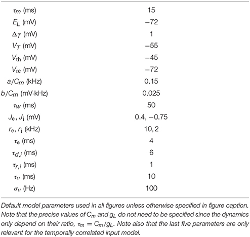
Table 1. Default parameter values.

We consider the neuron response statistics and the accuracy of our approximations under a variety of different parameter values. The “default” parameter values, used in all simulations except where explicitly stated otherwise in figure captions and axes labels, are given in Table 1.

For all Monte Carlo simulations, Equations (1–3) were solved using a forward Euler scheme with a time bin size of dt = 0.1 ms, except where specified otherwise. Each Monte Carlo simulation was of length 65 s. The first 5 s of all simulations were not used in computing statistics, so exactly 60 s were used. Statistics were computed by averaging over 10 such Monte Carlo simulations, except where specified otherwise. All simulations and numerical computations were performed on a MacBook Pro running OS X 10.11.2 with a 2.3 GHz Intel Core i7 processor and 16 GB of 1600 MHz DDR3 RAM. Simulations were run in Matlab R2015b (Mathworks) using the mex environment to compile C code that can be run from the Matlab command line.

2.2. A Review of Spectral and Statistical Measures of Stationary Stochastic Processes

We are interested in the steady-state statistics of membrane potential and spiking activity when the input current, I(t), is modeled as a stationary stochastic process. We first briefly review the statistical measures of stationary stochastic processes used in this study. A more in depth treatment can be found elsewhere (Yaglom, 2004; Tetzlaff et al., 2008). We model the spike train of a neuron as a sum of Dirac delta functions,

$s(t)={\displaystyle \sum _k\delta }(t-t_k)$

where t_k is the k-th threshold crossing of V(t). The steady-state firing rate is given by

$r_0=\underset{T\to \infty }{\lim }{T}^{-1}{\displaystyle {\int }_0^{T}s}(t)dt.$

A common measure of covariability between two processes is the cross-covariance function, defined by

$C_{XY}(\tau )=\text{cov}(X(t),Y(t+\tau ))$

for stationary stochastic processes, X(t) and Y(t). Analytical computations are often simplified by transitioning to the Fourier domain, defining the cross-spectral density,

${\tilde{C}}_{XY}(f)={\displaystyle {\int }_{-\infty }^{\infty }{C}_{XY}}(\tau )e^{-2\pi if\tau }d\tau$

and the power spectral density, ${\tilde{C}}_{XX}(f)$. The analytical and numerical computation of cross-spectral densities is simplified by the relationship (Yaglom, 2004),

${\tilde{C}}_{XY}(f)=\underset{T\to \infty }{\lim }{\tilde{X}}_T^{*}(f){\tilde{Y}}_T(f)$

where * denotes the complex conjugate,

$\begin{array}{ll}{\tilde{X}}_T(f)=\frac{1}{\sqrt{2T}}{{\displaystyle \int }}_{-T}^T[X(t)-{\mu }_X]e^{-2\pi ift}dt\hfill & (5)\hfill \end{array}$

is the normalized, finite-time Fourier transform of X(t) with its steady-state mean, μ_X, subtracted and similarly for Y_T(t). This relationship is particularly useful because it allows convolutions to be treated easily. In particular, suppose that U(t) = (K*X)(t) where * denotes convolution and K(t) is a deterministic kernel with finite L² norm. Then

$\begin{array}{ll}{\tilde{U}}_T(f)=\tilde{K}(f){\tilde{X}}_T(f)\hfill & (6)\hfill \end{array}$

for sufficiently large T where

$\tilde{K}(f)={\displaystyle {\int }_{-\infty }^{\infty }K}(t)e^{-2\pi ift}dt$

is the Fourier transform of K(t), and therefore

$\begin{array}{ll}{\tilde{C}}_{UU}(f)=|\tilde{K}(f){|}^2{\tilde{C}}_{XX}(f).\hfill & (7)\hfill \end{array}$

Finally, the steady-state variance can be computed from the integral of the power-spectral density,

$\begin{array}{ll}\text{var}(X)={\displaystyle {\int }_{-\infty }^{\infty }{\tilde{C}}_{XX}(f)df}\hfill & (8)\hfill \end{array}$

These relationships will be helpful in computing several statistics used below.

3. Results

3.1. A Review of the Quasi-Static Approximation for Stochastic Neuron Models with Adaptation Currents

We first consider the AdEx model from Equations (1–3) with temporally uncorrelated inputs. In this case, a classic diffusion approximation (Gluss, 1967; Capocelli and Ricciardi, 1971; Ricciardi and Sacerdote, 1979) replaces I(t) from Equations (4) with

$\begin{array}{ll}I(t)={\mu }_I+\sqrt{2D_I}\eta (t)\hfill & (9)\hfill \end{array}$

where μ_I = J_er_e + J_ir_i is the mean input bias,

$\begin{array}{ll}{D}_I=\frac{J_{\text{e}}^2{r}_{\text{e}}+J_{\text{i}}^2{r}_{\text{i}}}{2}\hfill & (10)\hfill \end{array}$

is the effective diffusion coefficient and η(t) is standard Gaussian white noise. This choice of coefficients, μ_I and D_I, assures that the steady-state mean of the input current is captured exactly by the input model and also that the first two infinitesimal moments of the membrane potential are the same for the diffusion approximation as they are for the temporally uncorrelated input model (Gluss, 1967; Capocelli and Ricciardi, 1971; Ricciardi and Sacerdote, 1979).

Under the diffusion approximation in Equations (9), the AdEx model from Equations (1–3) represents a coupled, two-dimensional system of stochastic differential equations. Therefore, the joint probability density of V and w obeys a two-dimensional Fokker-Planck equation (see Hertäg et al., 2014 for full formulation of the two-dimensional Fokker-Planck equation). In principle, this equation could be solved numerically and the resulting bivariate probability density could be used to compute the firing rate of the neuron. However, the Fokker-Planck equation is computationally expensive and difficult to solve, in part because it has two spatial dimensions and in part because of the non-local boundary conditions associated with the threshold-reset condition in Equation (3) (Richardson, 2009; Hertäg et al., 2014; Ocker and Doiron, 2014).

Previous studies of stochastic neuron models with voltage-activated adaptation currents (Richardson, 2009; Hertäg et al., 2014; Ocker and Doiron, 2014) resolve the difficulty inherent in solving a two-dimensional equation by utilizing the fact that the adaptation time constant, τ_w, is typically much larger than the membrane time constant, τ_w ≫ τ_m = C_m∕g_L. This separation of timescales justifies a quasi-static approximation in which w in Equation (1) is replaced by its steady-state mean value, μ_w. Under this approximation, the AdEx model can be viewed as a non-adaptive exponential integrate-and-fire model (EIF, obtained by setting a = b = 0) with an extra bias term accounting for the mean adaptation current. The only difficulty is that the steady-state mean adaptation current depends on the steady-state firing rate and steady state mean membrane potential, and vice versa. In Richardson (2009) and Ocker and Doiron (2014), this difficulty was overcome by numerically computing the fixed point of their dependence as described next.

The linearity of Equation (2) allows the steady-state mean value of w(t) to be computed exactly in terms of the firing rate and the steady state mean of V(t). Specifically, taking expectations in Equation (2) and including the spike-based perturbations from Equation (3) gives,

$\begin{array}{ll}{\tau }_w\frac{d\langle w\rangle }{dt}=a(\langle V\rangle -E_L)-\langle w\rangle +{\tau }_{w}br\hfill & (11)\hfill \end{array}$

where 〈w〉 is the time-dependent mean of w(t), 〈V〉 is the time-dependent mean membrane potential and r(t) is the instantaneous firing rate of the neuron. The last term in this equation captures the fact that w(t) is incremented by b each time the neuron spikes, as indicated in Equation (3). The steady-state mean is given by finding the unique fixed point of this differential equation,

$\begin{array}{ll}\begin{array}{l}{\mu }_w=\underset{t\to \infty }{\lim }\langle w\rangle \hfill \\ =a({\mu }_V-E_L)+{\tau }_{w}b{r}_0\hfill \end{array}\hfill & (12)\hfill \end{array}$

where μ_V and r₀ are the steady-state mean membrane potential and firing rate respectively.

Once w(t) is replaced by its steady-state mean value and I(t) is replaced by Gaussian white noise plus a bias term, μ_I, Equation (1) is a one-dimensional stochastic differential equation,

$\begin{array}{ll}\begin{array}{l}{C}_m\frac{dV}{dt}=g_L(E_L-V)+\psi (V)\hfill \\ -{\mu }_w+{\mu }_I+\sqrt{2D_I}\eta (t),\hfill \\ V\ge V_{\text{th}}\Rightarrow V\to V_{\text{re}}.\hfill \end{array}\hfill & (13)\hfill \end{array}$

Thus, the steady-state probability density of V and the steady state firing rate can be computed by solving a time-independent Fokker-Planck equation, parameterized by μ_w (see Appendix A for precise formulation of the one-dimensional Fokker-Planck equation).

This Fokker-Planck equation can be solved numerically efficiently using the threshold integration method developed in Richardson (2007, 2008). We improved computational efficiency of previous implementations of the threshold integration method in several ways. First, we implemented the solver in the C programming language. To maintain usability, we used the Matlab “mex” environment so that the compiled C code can be called from the Matlab command line. Additionally, solver allows for a variable mesh size so that the mesh can be refined where the derivative of the solution is expected to be large in magnitude.

Finally, we improved the numerical scheme used to implement the threshold-integration method. Previous implementations used a “modified Euler scheme” that exploits the linearity of the Fokker-Planck equation to write the solution in terms of integrals over mesh elements (Richardson, 2008). Whereas these previous implementations used the midpoint rule to approximate the resulting integrals, we used the more accurate Simpson's rule. A detailed description of the numerical solver is given in Appendix A. The performance of our implementation is compared to previous implementations below.

In summary, the mean membrane potential and firing rate, μ_V and r₀, can be computed as a function of the mean adaptation current, μ_w, by numerically solving the Fokker-Planck equation. Similarly, the steady-state mean of the adaptation variable can be computed in terms of the steady-state mean membrane potential and firing rate using Equation (12). Combining these two strategies, the steady state statistics can be approximated using fixed point iteration (see Appendix B). We hereafter refer to the approximation obtained this way as the “quasi-static approximation” to steady-state statistics. This approach was used previously in Richardson (2009) and Ocker and Doiron (2014).

The quasi-static approximation is expected to be accurate when adaptation is slow and weak (Richardson, 2009; Ocker and Doiron, 2014). We tested the accuracy of the quasi-static approximation with stronger and fast adaptation (see Methods) as a function of the the rate, r_e, of excitatory presynaptic spikes (Figure 1). While the quasi-static approximation captured the overall shape of the dependence of steady state firing rate on r_e (Figure 1A, compare red circles and gray curve), the errors were substantial in magnitude and percentage (Figures 1B,C, gray curve).

FIGURE 1

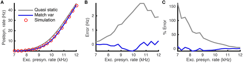
Figure 1. Quasi-static and matched variance approximations to the firing rate of an adaptive neuron model compared to Monte Carlo simulations as a function of presynaptic input rate. (A) Steady-state postsynaptic Firing rate, r₀, as the presynaptic excitatory rate, r_e, increases. Plotted for Monte-Carlo simulations (red circles), quasi-static approximation (gray curve) and matched variance approximation (blue curve). (B,C) Error and % error of the quasi-static and matched variance approximations compared to Monte-Carlo simulations. The temporally uncorrelated input model was used with all parameters except r_e given in Table 1.

We next show that these errors are due largely to the fact that the quasi-static approximation does not account for sub-threshold, passive membrane potential variability elicited by sub-threshold, voltage-based adaptation. We then propose an improved approximation that accounts for this variability.

3.2. A Matched Variance Approximation to Sub-Threshold Adaptation Dynamics

We conjectured that the errors made by the quasi-static approximation were largely due sub-threshold fluctuations in w(t), which are not accounted for by the quasi-static approximation. Our goal in this section is to derive a diffusion approximation that accurately captures the steady-state free membrane potential variance when sub-threshold adaptation is taken into account.

To demonstrate the source of the errors made by the quasi-static approximation, first consider the free membrane potential under the quasi-static approximation, defined by removing active currents and spiking from Equation (13) to obtain

$\begin{array}{l}{C}_m\frac{dU}{dt}=g_L(E_L-U)-{\mu }_w\\ -{\mu }_I+\sqrt{2D_I}\eta (t).\end{array}$

This represents an Ornstein-Uhlenbeck process with steady-state variance (Gardiner, 1985)

$\begin{array}{ll}\text{var}(U)=\frac{D_I{\tau }_m}{C_m^2}.\hfill & (14)\hfill \end{array}$

where τ_m = C_m∕g_L. Thus, the variance of the free membrane potential under the quasi-static approximation does not depend on adaptation dynamics at all (since Equation 14 does not depend on μ_w, τ_w, a or b).

For the full AdEx model, the sub-threshold membrane potential is affected by fluctuations in w(t) through voltage-based adaptation. This can be seen by considering the free membrane potential and adaptation dynamics defined by omitting spike-activation and spiking dynamics from Equations (1–3) to obtain

$\begin{array}{ll}\begin{array}{l}{C}_m\frac{dU}{dt}=-g_L(U-E_L)-W+I\\ {\tau }_w\frac{dW}{dt}=-W+a(U-E_L).\end{array}\hfill & (15)\hfill \end{array}$

Here, U(t) represents the free membrane potential and W(t) the “free adaptation” current. Since these equations are coupled, fluctuations in W(t) affect fluctuations in V(t) and vice versa.

In Appendix C, we show that the steady-state variance of U(t) under Equations (15) for the temporally uncorrelated input model is given by

$\begin{array}{ll}\text{var}(U)=\frac{D_I{\tau }_m}{C_m^2}\left[1-\left(\frac{a}{a+g_L}\right)\left(\frac{{\tau }_m}{{\tau }_m+{\tau }_w}\right)\right]\hfill & (16)\hfill \end{array}$

where $D_I=(J_{\mathrm{\text{e}}}^2{r}_{\mathrm{\text{e}}}+J_{\mathrm{\text{i}}}^2{r}_{\mathrm{\text{i}}})∕2$ as above. This reveals a major source of error in the quasi-static approximation. As noted above, the free membrane potential variance for the quasi-static approximation (Equation 14) does not depend on adaptation at all. On the other hand, the free membrane potential variance of the full model is affected by sub-threshold adaptation currents, since Equation (16) depends on a and τ_w. Comparing Equations (14) and (16) reveals that the steady-state variance under the quasi-static approximation is least accurate when adaptation is strong (a larger relative to g_L) and/or fast (τ_w smaller relative to τ_m).

This difference is demonstrated by comparing the approximated and actual free membrane potential variance for different values of a and τ_w (Figure 2). The quasi-static approximation does especially poorly in capturing the free membrane potential variability when a is large or τ_w is small (Figure 2B). These errors in approximating the variability of sub-threshold membrane potential variability introduce errors in the resulting firing rate approximation. Notably, the percent error made in approximating the firing rate depends similarly on the adaptation parameters as the percent error made in approximating the membrane potential variance (Figures 3C,D, compare to Figure 2B).

FIGURE 2

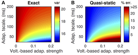
Figure 2. Steady-state free membrane potential variance and the error in estimating it with a quasi-static approximation. (A) Steady-state free membrane potential variance when sub-threshold adaptation is accounted for, from Equation (16), as a function of voltage-based adaptation strength, a, and adaptation timescale, τ_w. (B) Percent error of quasi-static approximation to the steady-state membrane potential variance, from Equation (14), vs. the variance from (A). Adaptation strengths, a, are reported in units kHz·C_m. Voltage variance has units mV². All parameters other than a and τ_w are as in Table 1.

FIGURE 3

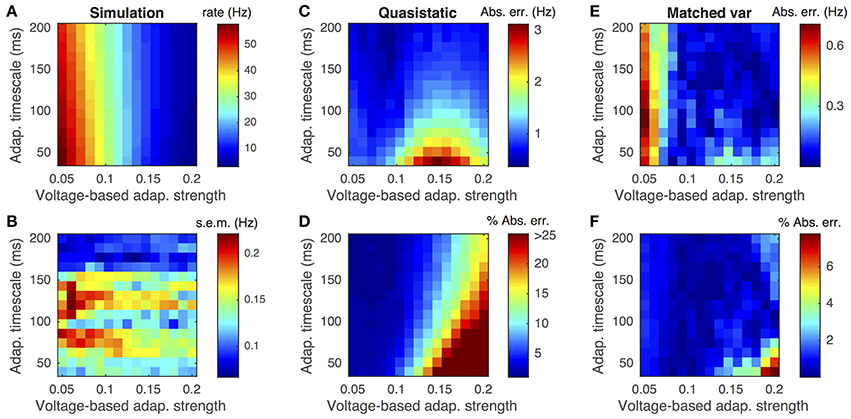
Figure 3. Firing rate approximations and errors as a function of voltage-based adaptation strength and timescale. (A) Firing rate from Monte-Carlo simulations as a function of voltage-based adaptation strength, a, and adaptation timescale, τ_w. (B) Standard error of the mean from simulations in (A). (C,D) Absolute error and percent absolute error of quasi-static approximation to firing rate compared to simulations from (A). (E,F) Same as (C,D), but for matched variance approximation. Adaptation strengths, a, are reported in units kHz·C_m. The temporally uncorrelated input model was used. All parameters other than a and τ_w are as in Table 1.

We now derive a one-dimensional “matched variance” diffusion approximation that accurately captures the steady-state free membrane potential variance of the two-dimensional model in Equation (15). This diffusion approximation is defined by

$\begin{array}{ll}\begin{array}{l}{C}_m\frac{dU}{dt}=-g_L(U-E_L)-{\mu }_w+{\mu }_I\hfill \\ +\sqrt{2D_{\text{eff}}}\eta (t)\hfill \end{array}\hfill & (17)\hfill \end{array}$

where η(t) is standard Gaussian white noise and the diffusion coefficient, D_eff, is scaled to account for the variability of V(t) in the presence of sub-threshold adaptation. The steady-state free membrane potential variance from Equation (17) is Gardiner (1985)

$\begin{array}{ll}\text{var}(U)=\frac{D_{\text{eff}}{\tau }_m}{C_m^2}.\hfill & (18)\hfill \end{array}$

We want to choose D_eff so that this variance is equal to the variance in Equation (16) from the two-dimensional model. This is achieved by setting Equation (16) equal to Equation (18) and solving for D_eff to obtain

$\begin{array}{ll}{D}_{\text{eff}}=D_I\left[1-\left(\frac{a}{a+g_L}\right)\left(\frac{{\tau }_m}{{\tau }_m+{\tau }_w}\right)\right]\hfill & (19)\hfill \end{array}$

where $D_I=(J_{\mathrm{\text{e}}}^2{r}_{\mathrm{\text{e}}}+J_{\mathrm{\text{i}}}^2{r}_{\mathrm{\text{i}}})∕2$. This choice of D_eff defines the “matched variance” approximation under the temporally uncorrelated input model (see Methods).

In summary, the matched variance diffusion approximation, given by using Equation (17) with D_eff from Equation (19), achieves the same steady state free membrane potential variance as the two-dimensional model in Equation (15) under the temporally uncorrelated input model (see Methods). This approach is similar to previous matched variance approximations that account for the effects of temporally correlated noise, but not sub-threshold adaptation, on the free membrane potential variance (Alijani and Richardson, 2011; Hertäg et al., 2014). Below, we consider a combination of these approaches that accounts for both voltage-based adaptation and temporally correlated inputs.

Once D_eff is computed, the matched variance approximation to the firing rates can be computed using the same Fokker-Planck solver and iterative methods used for the quasi-static approximation reviewed above and in Appendices A and B. The only difference between the quasi-static and matched variance approximations is the choice of diffusion coefficient, D_I or D_eff.

The matched variance diffusion approximation corrects a substantial portion of the error made by the quasi-static approximation, especially when the neuron is in the fluctuation dominated regime (Figure 1, compare blue and gray). This is because the fluctuations introduced by the adaptation current alter firing rates the most in the fluctuation driven regime.

Moreover, the matched variance approximation provides a substantially improved firing rate approximation whenever voltage-based adaptation is strong and/or fast (a large, τ_w small; Figures 3E,F). Notably, the absolute error in firing rate is less than 1 Hz and the relative error less than 10% for the entire set of parameters we considered (Figures 3E,F). It was greater than 1 Hz and 10% for a considerable portion of the parameters using the quasi-static approximation (Figures 3C,D). Nevertheless, the matched variance approximation replaces the temporally correlated adaptation current with white noise which introduces some error, especially when adaptation is strong and fast (Figure 3F).

The matched variance approximation offers essentially the same computational efficiency as the quasi-static approximation since they only differ by the value of the diffusion coefficient used. The average CPU time used to compute each firing rate data point in Figure 1 was 1.4 ms for the quasi-static approximation and 1.5 ms for the matched variance approximation.

A comparison of numerical schemes for solving the Fokker-Planck equation shows that the modified Euler scheme with Simpson's rule substantially outperforms the previously proposed modified Euler scheme with the midpoint rule (Figure 4, compare blue and red). Interestingly, a standard Euler scheme slightly outperforms the modified Euler scheme with the midpoint rule (Figure 4, compare green and red), but only gives a reasonable approximation for very fine meshes, due to the large exponential nonlinearity in ψ(V) for V near V_T (Richardson, 2008).

FIGURE 4

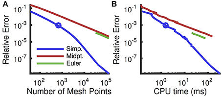
Figure 4. Convergence of numerical schemes for computing steady state firing rate. (A) Relative numerical error (defined as the relative deviation of the computed firing rate from the rate computed with a fine uniform mesh of size dv = 10⁻⁴ mV which gives 7 × 10⁵ mesh points) plotted as a function of the number of mesh points. The mesh was uniform except near V_re and V_th where it was refined (see Appendix A). (B) Same error plotted as a function of CPU time to compute the firing rate. Firing rates were computed using the threshold integration method with a standard Euler solver (green), the modified Euler method from Richardson (2007, 2008) using a midpoint rule for integration (red) and the modified Euler method using Simpson's rule (blue). For the Euler method, the error is not plotted for coarser meshes because they yielded a predicted firing rate of zero. Circle indicates the mesh size used in all other figures. All parameters are as in Table 1.

Despite the fact that the matched variance approximation captures some of the variability introduced by sub-threshold voltage-based adaptation, errors are introduced by several assumptions made by the model. We next explore these other sources of error by modulating various parameters of the model.

Both the quasi-static and matched variance approximations approximate spike-based inputs with Gaussian white noise. This diffusion approximation is only mathematically valid in the limit of small synaptic weights, J_e, J_i ≪ 1, and large presynaptic firing rates, r_e, r_i ≫ 1 (Ricciardi and Sacerdote, 1979). To test the dependence of our numerical approximations on the synaptic weights, we computed the error in approximating postsynaptic firing rates as the synaptic weights were scaled and firing rates were scaled inversely, so that the mean input, μ_I = J_er_e + J_ir_i remained fixed. Specifically, we set J_x → cJ_x and r_x → r_x∕c for x = e, i and for a range of scalings, c. We found that the matched variance approximation accurately predicted the firing rate over a large range of scalings (Figure 5 blue curve, absolute error < 5% for all data points) and substantially outperforms the quasi-static approximation (Figure 5, compare blue and gray).

FIGURE 5

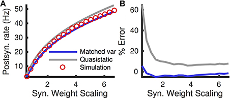
Figure 5. Firing rate and error as a function of synaptic weights. (A) Steady state firing rate from simulations (red circles), quasi-static approximation (gray) and matched variance approximation (blue) as synaptic weights, J_e and J_i, are scaled by different factors. (B) Percent errors from (A). Presynaptic firing rates, r_e and r_i, were scaled inversely so that μ_I = J_er_e+J_ir_i remained constant. The temporally uncorrelated input model was used. All parameters other than J_e, J_i, r_e and r_i are as in Table 1.

While the matched variance approximation corrects for some variability introduced by sub-threshold, passive adaptation, it does not correct for fluctuations in the adaptation current evoked by action potentials. Some of this variability is introduced the reset of the membrane potential after a spike, V → V_re. This reset rule affects the adaptation current, w, through the voltage-based adaptation. If V_re is far from the steady-state mean membrane potential, the voltage-reset rule has a larger impact on the adaptation current, so we expect the matched variance approximation to perform poorly since it ignores this impact altogether. Indeed, we found that the matched variance approximation performs especially poorly for V_re < −80 mV (Figure 6). Nevertheless, it still outperforms the quasi-static approximation (Figure 6, compare blue and gray).

FIGURE 6

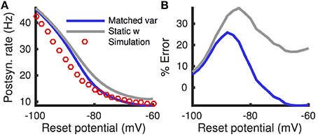
Figure 6. Firing rate and error as a function of reset potential. (A) Steady state firing rate from simulations (red circles), quasi-static approximation (gray) and matched variance approximation (blue) as a function of the reset potential, V_re. (B) Percent errors from (A). The temporally uncorrelated input model was used. All parameters other than V_re are as in Table 1.

Surprisingly, we found that a lower reset potential (V_re more negative) produced a larger firing rate, and this effect was captured by simulations and both numerical approximations (Figure 6A). This is a consequence of strong voltage-based adaptation. Resetting the membrane potential far below E_L also reduces the adaptation current, w, through Equation (2). The membrane potential recovers from its reset before w (since τ_m < τ_w), during which time the neuron has an increased likelihood of spiking.

While the matched variance approximation captures some sub-threshold fluctuations introduced by voltage-based adaptation, it uses the same approximation to the effects of spike-based adaptation that the quasi-static approximation uses. Thus, we expect both approximations to perform poorly when spike-based adaptation is too strong or fast. We confirmed this expectation by comparing both approximations to Monte-Carlo simulations over a range of spike-based adaptation strengths, b, and adaptation timescales, τ_w (Figure 7). As expected, the matched variance approximation performed most poorly when spike-based adaptation was both fast and strong (Figures 7E,F). The quasi-static approximation performed poorly for faster adaptation, but interestingly performed better for stronger spike-based adaptation (Figures 7C,D). Surprisingly, the quasi-static approximation actually performed better than the matched variance approximation for strong and slow spike-based adaptation.

FIGURE 7

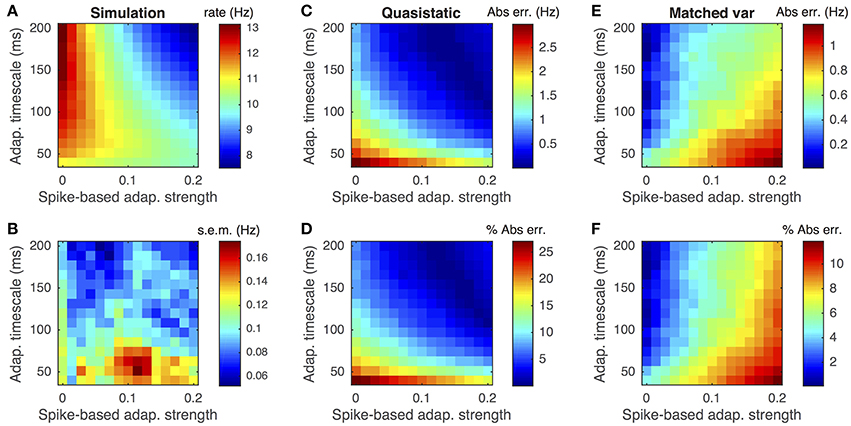
Figure 7. Firing rate approximations and errors as a function of spike-based adaptation strength and timescale. (A–F) Same as Figures 3A–F except that spike-based adaptation strength, b, was varied instead of voltage-based. Adaptation strengths, b, are reported in units mV·kHz·C_m. The temporally uncorrelated input model was used. All parameters other than a and τ_w are as in Table 1.

3.3. Numerical Methods to Compute the Linear Response to a Modulation of Input Current

So far, we considered numerical methods to compute the steady state firing rate of an adaptive model neuron with stationary inputs. We now consider the response of the neuron to inputs whose statistics exhibit an explicit time-dependence. In general, this would require solving a time-dependent formulation of the Fokker-Planck equation that is not amenable to the threshold-integration methods used for the steady state problem. However, if the temporal modulation of the statistics are weak, threshold-integration methods can be used to solve the time-dependent Fokker-Planck equation to first order in the magnitude of the modulation (Richardson, 2007, 2008). This can be combined with linear response theory to quantify neuronal signal transfer, inter-neuronal correlations and recurrent network stability (Lindner et al., 2005; de la Rocha et al., 2007; Richardson, 2008; Shea-Brown et al., 2008; Ostojic et al., 2009; Ledoux and Brunel, 2011; Trousdale et al., 2012). We follow previously developed methods for computing the response of an adaptive neuron model to a modulation (Richardson, 2009; Ocker and Doiron, 2014), with some refinements. Details of the implementation are given in Appendix D and we review the overall approach here.

In short, we consider a weak perturbation to the synaptic input of the form

$I(t)=I_0(t)+ϵu(t)$

where I₀(t) is the un-perturbed input considered above and u(t) is some stationary perturbation. Linear response theory can be used to show that the finite-time Fourier transform of the firing rate can be written as

${\tilde{r}}_T(f)=ϵS_r(f){\tilde{u}}_T(f)+o(ϵ)$

for sufficiently large T where ${\tilde{S}}_r(f)$ is the the susceptibility function of the neuron's firing rate (Risken, 1996; Fourcaud and Brunel, 2002).

The susceptibility function can be computed from a one-dimensional Fokker-Planck equation, linearly coupled with an equation for the modulation of the adaptation current. This can in turn be solved using threshold-integration methods. This approach was first developed in Richardson (2009) and also used in Ocker and Doiron (2014). We review the approach and our implementation of it in Appendix D. Similar to our computation of steady-state statistics, we improved the efficiency and accuracy of the susceptibility computation by implementing the solver in C, using Simpson's method to compute integrals and using the matched variance approximation for the effective diffusion coefficient.

It is often necessary to take an inverse Fourier transform of susceptibility functions (see the examples below, for instance). Using Fast Fourier Transform methods for this inverse requires a uniform grid of frequencies. This grid must be fine enough to capture the low-frequencies introduced by adaptation, but must also extend to sufficiently high frequencies to capture faster spiking and membrane potential timescales. As a result, the susceptibility functions must be evaluated at a large number of frequency values. This can be computationally expensive since threshold-integration must be performed separately for each value of f (see Appendix D).

To overcome this high computational cost, we note that susceptibility functions of neuron models are typically smooth and slowly varying functions of f, especially at higher frequencies and especially when viewed on a log-log scale (see Figure 8, for example). Instead of evaluating them at each value of f, we first evaluate them at a coarser, potentially non-uniform mesh of frequencies. Since the functions change more sharply at lower frequencies, we use a mesh that is uniform on a log scale. Once the susceptibility functions are computed on this coarser mesh, interpolation is used to estimate their values on a finer, uniform mesh. The inverse Fast Fourier Transform can then be applied to the interpolated values, since the mesh is uniform and sufficiently fine. We specifically found that using piecewise-cubic Hermite interpolating polynomials (Fritsch and Carlson, 1980) via Matlab's built-in pchip command yields accurate results when the coarser mesh has only 30 points (spaced evenly on a log scale). We next verify this numerical approach by approximating spike triggered averages and inter-neuronal spike train correlations, which require the application of an inverse transform to the susceptibility functions.

FIGURE 8

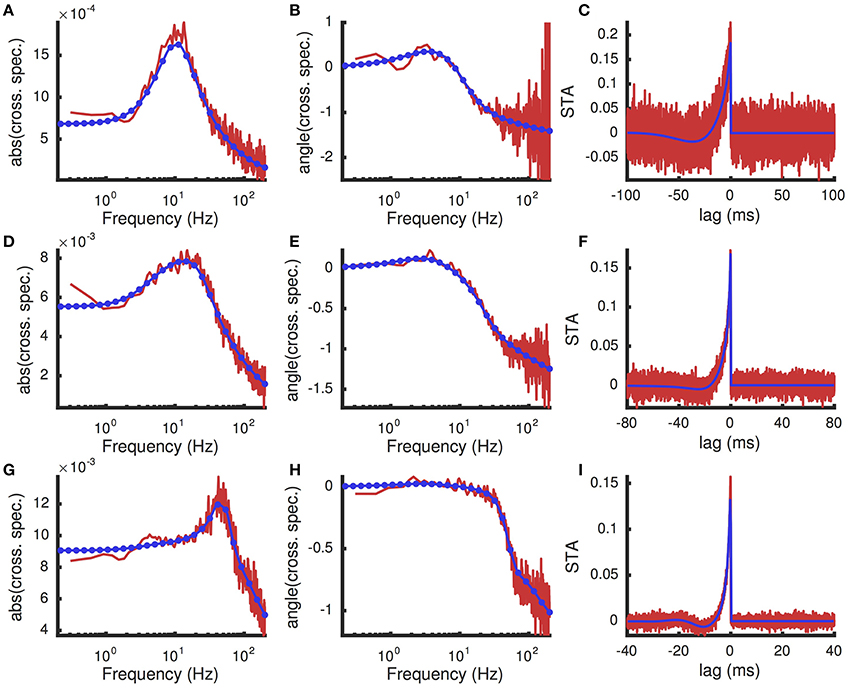
Figure 8. Spike triggered average input current and cross-spectral density under a white noise perturbation for different excitatory presynaptic rates. A weak white noise current was added to the model neuron ($D_n∕C_m^2=0.1$(mV)²/ms). (A,B) The magnitude ($\left|{\tilde{C}}_{us}\right|$ in units C_mmV) and phase ($\mathrm{\text{angle}}({\tilde{C}}_{us})$, in radians) of the cross-spectral density between the white noise input and postsynaptic spike train. (C) The spike triggered average (units C_mmV∕ms) of the white noise input. (A–C) were computed with presynaptic excitatory rate r_e = 8 kHz. (D–F) are the same as (A–C), but with r_e = 10 kHz. (G–I) are the same, but with r_e = 12 kHz. In all panels, results from Monte Carlo simulations are in red and numerical results from the matched variance approximation are in blue. The filled blue circles in indicate the coarse frequency values at which threshold-integration was applied. The smooth blue curve indicates the interpolated values used to compute the inverse Fourier transforms for the STAs. The temporally uncorrelated input model was used with the additional white noise input. All parameters except r_e are as in Table 1.

3.4. Computing Spike-Triggered Average and Cross-Spectral Density between the Spike Train and an Input Current Perturbation

To test the accuracy of our approximation of the response to a modulation, we performed Monte-Carlo simulations with a weak Gaussian white noise term was added to I(t),

$I(t)\to I(t)+u(t)$

where

$u(t)=\sqrt{2D_n}{\eta }_n(t)$

and η_n(t) is Gaussian white noise. The excitatory and inhibitory conductances were left un-perturbed for this example.

We considered two ways to quantify the response to the white noise perturbation. We first considered the cross-spectral density, ${\tilde{C}}_{us}(f)$, between the white noise input and the postsynaptic spike train (see Methods for definition). A direct application of linear response theory shows that the cross-spectral density is given to first order in D_n by

${\tilde{C}}_{us}(f)=2D_n{S}_r(f).$

Thus, the cross-spectral density can be numerically approximated by computing the susceptibility function. We also considered the spike-triggered average noise, defined by

$STA(\tau )={\text{avg}}_j\left(u(\tau -t_j)\right)$

where t_j are the spike times of the neuron. These STA can be computed from the cross-spectral density by first noting that (Dayan and Abbott, 2001)

$STA(\tau )=\frac{C_{us}(-\tau )}{r_0}$

where C_us(τ) = cov(u(t), s(t + τ)) is the cross-covariance function between the white noise input and the postsynaptic spike train, which is the inverse Fourier transform of ${\tilde{C}}_{us}(f)$ (see Methods and Tetzlaff et al., 2008). Putting this all together gives

$STA=\frac{2D_n}{r_0}{ℱ}^{-1}\left[S_r^{*}\right]$

where ${F}$⁻¹ denotes the inverse Fourier transform and * the complex conjugate. Thus, the spike-triggered average can be approximated directly from the susceptibility through an inverse Fourier transform of the susceptibility function.

A comparison of the numerically computed values of STA(τ) and ${\tilde{C}}_{us}(f)$ to their estimates from Monte-Carlo simulations of the full AdEx model shows good agreement (Figure 8). Note that, since the cross-spectral density is proportional to the susceptibility, Figure 8 also reveals the shape of the susceptibility function and demonstrates the interpolation used (compare coarse mesh indicated by blue circles to interpolated fine mesh indicated by solid blue curve). The peak in the susceptibility function arises from resonance inherited by the spike- and voltage-based adaptation rules (Brunel et al., 2003; Richardson et al., 2003; Richardson, 2009; Ocker and Doiron, 2014). This resonance is captured by the numerical approximation because the fixed point computation of the susceptibility function takes into account the linear filtering of the adaptation currents (see Appendix D) as in Richardson (2009) and Ocker and Doiron (2014). Computing the numerical approximation to the cross-spectral density and spike triggered average over a larger range of presynaptic excitatory rates, r_e shows that this peak is a robust feature of the adaptive model at various firing rates (Figure 9).

FIGURE 9

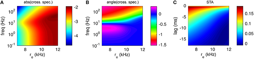
Figure 9. Spike triggered average input current and cross-spectral density under a white noise perturbation as a function of presynaptic excitatory rate. Same as Figure 8 except that only numerical results are shown, using the matched variance approximation, over a range of values of the excitatory presynaptic rate, r_e.

Numerical computation of the linear response function, cross-spectrum and spike triggered average was extremely efficient, with all three computed in 21 ms on average for each value of r_e used in Figure 9. As noted above, this efficiency was obtained by first computing S_r(f) at a coarse and non-uniform mesh of frequencies, then using polynomial interpolation to approximate the response at a fine, uniform grid of frequencies so that the inverse Fast Fourier Transform can be used to calculate STA(τ). Using this approach, the threshold-integration scheme was only called 30 times (one for each coarse frequency mesh point), but capturing the fast and slow timescales in STA(τ) required interpolating these 30 values to a fine mesh of 20,001 frequency values (0 to 2 kHz with 0.1 Hz steps). To estimate the efficiency added by our interpolation scheme, we tried computing the susceptibility directly on the finer mesh (with r_e = 10 kHz). This required 20,001 calls to the threshold-integration scheme and took 2.5 s. Thus, our interpolation approach is about 100 times faster than computing the susceptibility at each frequency directly.

3.5. Computing the Cross-Covariance Function between the Spiking Response of Two Model Neurons

We now consider two identical versions of the pyramidal neuron model, each identical to the individual models considered above, but with the additional assumption that a proportion c = 0.1 of the excitatory presynaptic spike times are shared between the neurons. This scenario models two neurons with overlapping presynaptic pools. These shared presynaptic spikes introduce correlations between the inputs to the two neurons, which in turn introduces correlations between their postsynaptic spike trains,

$s_k(t)={\displaystyle \sum _j\delta }(t-t_{k,j})$

where t_{k, j} is the jth spike of neuron k = 1, 2.

Linear response theory can be used to show that the cross-spectral density is given to first order in c by Lindner et al. (2005), de la Rocha et al. (2007), and Shea-Brown et al. (2008)

${\tilde{C}}_{s_1{s}_2}(f)=|S_r(f){|}^2{\tilde{C}}_{I_1{I}_2}(f)$

where S_r(f) is the susceptibility function of both neurons and

${\tilde{C}}_{I_1{I}_2}(f)=c{J}_{\text{e}}^2{r}_{\text{e}}$

is the cross-spectral density between the neurons' input currents. The cross-covariance can then be computed through an inverse Fourier transform of the cross-spectral density (see Methods).

Comparing the cross-covariance and cross-spectral density approximated numerically using this method to those computed from Monte-Carlo simulations shows reasonable agreement (Figure 10). Moreover, the numerical approximations were computed efficiently, taking less than 50 ms.

FIGURE 10

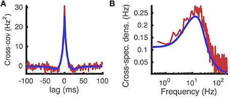
Figure 10. Cross-covariance between two identical neurons receiving shared excitatory synaptic input. (A) Cross-covariance and (B) cross-spectral density between the spike trains produced by two identical AdEx model neurons that share 10% of their excitatory presynaptic spike times, which occur as a homogeneous Poisson process. Computed from Monte Carlo simulations (red) and from the matched variance approximation (blue). The temporally uncorrelated input model was used. All parameters are as in Table 1.

An analogous approach can be applied when the neurons share inhibitory presynaptic inputs too. Moreover, an extension of this method can be applied to compute the correlation between synaptically coupled neurons and the entire matrix of cross-correlations in large, sparsely coupled networks (Ostojic et al., 2009; Trousdale et al., 2012). Thus, our numerical methods can be used to efficiently approximate the correlation structure of large populations of synaptically coupled adaptive model neurons.

3.6. A Matched Variance Approximation with Temporally Correlated Input Currents

So far we have considered numerical approximations obtained for a model of temporally uncorrelated synaptic input currents (see Methods). Synaptic currents in vivo are temporally correlated due to synaptic kinetics and temporal correlations in presynaptic spike timing. This shortcoming has been partially overcome by approximations that scale the diffusion coefficient to capture the steady-state free membrane potential variance of the full model (Alijani and Richardson, 2011; Hertäg et al., 2014), analogous to the matched variance approximation to adaptation dynamics described above. In these previous approaches, the approximation was only applied to synaptic input currents with an exponentially-shaped auto-correlation function, which can be used to model Poisson presynaptic spiking with exponential post-synaptic current waveforms. Moreover, these previous approaches were either applied to non-adaptive neuron models (Alijani and Richardson, 2011) or did not account for the effects of sub-threshold adaptation on the free membrane potential variance (Hertäg et al., 2014). We next extend this approach to account for sub-threshold adaptation and arbitrary stationary stochastic input.

First note that the linearity of Equations (15) allows the steady-state variance of U(t) to be computed for any stationary input I(t). Specifically, note that each line in Equation (15) implements a linear filter so that, for sufficiently large t,

$\begin{array}{ll}\begin{array}{l}U(t)=(K_v*I)(t)-(K_v*W)(t)+c_1(t)\hfill \\ W(t)=a(K_w*U)(t)+c_2(t)\hfill \end{array}\hfill & (20)\hfill \end{array}$

where c₁(t) and c₂(t) are asymptotically constant as t → ∞ and * denotes convolution. The kernels of the membrane potential and adaptation filters are given by

$K_v(t)=\frac{1}{C_m}{e}^{-t/{\tau }_m}\Theta (t),$

and

$K_w(t)=\frac{1}{{\tau }_w}{e}^{-t/{\tau }_w}\Theta (t),$

where τ_m = C_m∕g_L and Θ(t) is the Heaviside step function. Transitioning to the Fourier domain and using Equation (6), we can write Equations (20) as

$\begin{array}{l}{\tilde{U}}_T(f)={\tilde{K}}_v(f){\tilde{I}}_T(f)-{\tilde{K}}_v(f){\tilde{W}}_T(f)\\ {\tilde{W}}_T(f)=a{\tilde{K}}_w(f){\tilde{U}}_T(f)\hfill \end{array}$

for sufficiently large T where

${\tilde{K}}_v(f)=\frac{{\tau }_m}{C_m(1+2\pi if{\tau }_m)}$

and

${\tilde{K}}_w(f)=\frac{1}{1+2\pi if{\tau }_w}$

are the Fourier transforms of K_v(t) and K_w(t). Here, ${\tilde{U}}_T(f)$, ${\tilde{I}}_T(f)$ and ${\tilde{w}}_T(f)$ are defined by Equation (5). This is a linear system of algebraic equations that is easily solved at each frequency, f, to obtain

${\tilde{U}}_T(f)=\frac{{\tilde{K}}_v(f)}{1+a{\tilde{K}}_v(f){\tilde{K}}_w(f)}{\tilde{I}}_T(f).$

The power spectral density of U(t) is therefore given by (see Equation 7)

$\begin{array}{l}{\tilde{C}}_{UU}(f)=\underset{T\to \infty }{\lim }|{\tilde{U}}_T(f){|}^2\hfill \\ =\frac{|{\tilde{K}}_v(f){|}^2}{|1+a{\tilde{K}}_v(f){\tilde{K}}_w(f){|}^2}{\tilde{C}}_{II}(f)\hfill \end{array}$

where ${\tilde{C}}_{II}(f)$ is the power spectral density of I(t). The steady-state variance of the free membrane potential is then given by

$\text{var}(U)={\displaystyle {\int }_{-\infty }^{\infty }{\tilde{C}}_{II}(f)|K_{\text{eff}}(f){|}^{2}df.}$

This expression is valid for any stationary input, I(t), for which ${\tilde{C}}_{II}(f)$ is defined and well-behaved (Yaglom, 2004).

Under the diffusion approximation in Equation (17), the free membrane potential variance is given by Equation (18). Combining these expressions shows that the diffusion approximation accurately captures the free membrane potential variance by taking

$\begin{array}{ll}{D}_{\text{eff}}=\frac{C_m^2}{{\tau }_m}{\displaystyle {\int }_{-\infty }^{\infty }{\tilde{C}}_{II}(f)|K_{\text{eff}}(f){|}^{2}df}\hfill & (21)\hfill \end{array}$

which defines the matched variance approximation to temporally correlated inputs. In the absence of voltage-based adaptation (a = 0) and when I(t) has an exponential-shaped auto-covariance function, this approximation is identical to the ones in Alijani and Richardson (2011) and Hertäg et al. (2014).

We consider an input model where temporal correlations are introduced by synaptic kinetics and by temporal correlations in the timing of presynaptic spikes (see Methods). Under this input model, the power spectral density of the synaptic input current is given by Rosenbaum et al. (2012b)

$\begin{array}{l}{\tilde{C}}_{II}(f)=J_{\text{e}}^2[r_{\text{e}}+{\tilde{C}}_{\nu \nu }(f)]{\tilde{\alpha }}_{\text{e}}(f)\\ +J_{\text{i}}^2[r_{\text{i}}+{\tilde{C}}_{\nu \nu }(f)]{\tilde{\alpha }}_{\text{i}}(f)\end{array}$

where

${\tilde{\alpha }}_{\text{e}}(f)=\frac{1}{1+4{\pi }^2{\tau }_{\text{e}}^2{f}^2}$

is the Fourier transform of the excitatory postsynaptic current waveform,

${\tilde{\alpha }}_{\text{i}}(f)=\frac{1}{(1+4{\pi }^2{\tau }_{r,\text{i}}^2{f}^2)(1+4{\pi }^2{\tau }_{d,\text{i}}^2{f}^2)}$

is the Fourier transform of the excitatory postsynaptic current waveform and

${\tilde{C}}_{\nu \nu }(f)=\frac{2{\sigma }_{\nu }^2{\tau }_{\nu }}{1+4{\pi }^2{\tau }_{\nu }^2{f}^2}$

is the power spectral density of the firing rate fluctuations, ν(t). Under this model, the integral in Equation (21) can be approximated numerically (we used the integral command in Matlab) to obtain the corrected diffusion coefficient that defines the matched variance approximation.

Testing this matched variance approximation against Monte-Carlo simulations shows that it captures the overall shape of the dependence of firing rate on presynaptic excitatory rate (Figure 11A, compare blue and red), but introduces large errors (Figures 11B,C blue). Nevertheless, it substantially out-performs the quasi-static approximation obtained using the diffusion coefficient in Equation (10) (Figures 11B,C gray).

FIGURE 11

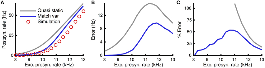
Figure 11. Quasi-static and matched variance approximations to firing rates when input currents are temporally correlated. (A) Steady-state postsynaptic Firing rate, r₀, as the presynaptic excitatory rate, r_e, increases. Plotted for Monte-Carlo simulations (red circles), quasi-static approximation (gray curve) and matched variance approximation (blue curve) for the temporally correlated input model (see Methods). (B,C) Error and % error of the quasi-static and matched variance approximations compared to Monte-Carlo simulations. The temporally correlated input model was used. All parameters other than r_e are as in Table 1.

The timescale of temporal input correlations is determined by the timescale of firing rate fluctuations, τ_ν, as well as the timescales of synaptic kinetics, τ_e, τ_{r, i} and τ_{d, i}. In the limit that all of these timescales approach zero, the input is approximated accurately by the temporally uncorrelated model. Thus, we expect the matched variance approximation for temporally correlated inputs to be approximately as accurate as for temporally uncorrelated inputs when these timescales are small.

To test this prediction, we compared the matched variance (and quasi-static) approximation to Monte-Carlo simulations as the input timescales were scaled (Figure 12). As expected, the matched variance approximation performs well when input timescales are fast, but not when they are slow (Figure 12, blue curves). The quasi-static approximation, obtained using the diffusion coefficient in Equation (10), does not capture any dependence of the firing rate on the input timescales and performs worse than the matched variance approximation (Figure 12, compare blue and gray curves).

FIGURE 12

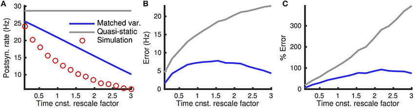
Figure 12. Firing rates and errors as a function of temporally correlated input timescale. (A) Steady state firing rate from simulations (red circles), quasi-static approximation (gray) and matched variance approximation (blue) as the timescales (τ_e, τ_{r, i}, τ_{d, i} and τ_ν) are scaled by different factors. (B,C) Errors and percent errors from (A). The excitatory presynaptic rate was increased to r_e = 11 kHz and the time bin width was decreased to dt = 0.05 for simulations. The temporally correlated input model was used. All parameters other than r_e, τ_e, τ_{r, i}, τ_{d, i} and τ_ν are as in Table 1.

These examples demonstrate that the matched variance approximation offers an improvement over approximations that do not correct for synaptic timescales at all, but there is substantial room for improvement in the approximation of firing rates of neuron models drive by temporally correlated inputs.

4. Discussion

We derived and tested a suite of accurate and efficient numerical methods for approximating the response statistics of the adaptive integrate-and-fire neuron models with noisy synaptic input. We introduced an extension of the matched variance approximation (Alijani and Richardson, 2011; Hertäg et al., 2014) to capture the effects of sub-threshold, voltage-based adaptation currents on passive membrane variability. This approximation is more accurate than previously posed quasi-static approximations to the effects of adaptation (Richardson, 2009; Ocker and Doiron, 2014), especially when voltage-based adaptation currents are strong and/or fast.

Our approximation is also applicable in the case of arbitrary, temporally correlated synaptic inputs. This extends previous approximations, which are applicable only when inputs have exponentially-shaped auto-correlations and which do not account for the effects of voltage-based adaptation currents on sub-threshold membrane potential variability (Alijani and Richardson, 2011; Hertäg et al., 2014). In the examples we considered, however, the matched variance approximation performed relatively poorly when strong adaptation was combined with temporally correlated inputs (Figures 11, 12).

The methods presented here rely heavily on previously developed techniques. The threshold-integration method was developed previously (Richardson, 2007, 2008) and we only improved the computational efficiency. Similarly, the fixed point iteration method for approximating the effect of an adaptation current was considered previously (Richardson, 2009; Ocker and Doiron, 2014) and we derived a re-scaled diffusion coefficient to account for variability in sub-threshold adaptation currents. A matched variance approximation has been developed to account for temporally correlated synaptic inputs and we extended this method to account for sub-threshold adaptation currents.

The response of model neurons to temporally correlated inputs has also been approximated using timescale separation when synaptic kinetics are much slower or faster than membrane dynamics (Moreno-Bote and Parga, 2006). However, with the exception of NMDA synaptic kinetics, synaptic and membrane timescales in cortex are not so separated, especially when one accounts for faster “effective” membrane time constant arising from the barrage of conductance-based inputs received by neurons in vivo (Destexhe and Paré, 1999; Destexhe et al., 2003; Kuhn et al., 2004).

Computational efficiency is often ignored when reporting on numerical methods for stochastic neuron models. We carefully designed our methods to be computationally efficient and tested this efficiency. As a consequence, our methods allow the computation of membrane potential response properties orders of magnitude faster than some previous methods for which timing has been reported (Hertäg et al., 2014), though our methods are potentially less accurate. While the difference between milliseconds and seconds of computation time is unimportant when computing the firing rate of a single neuron model for one set of parameters, it could be critical for applications where response properties need to be computed many times. For example, computing rates and correlations in a large recurrent network requires solving a fixed point point problem in which stationary rates and susceptibility functions are computed many times per neuron (Amit and Brunel, 1997; Brunel and Hakim, 1999; Trousdale et al., 2012). Additionally, fitting a network model to recorded multicellular data can require the repeated evaluation of rates and susceptibility functions for several parameter values and several neurons (Pernice and Rotter, 2013).

Our methods compromise some accuracy for biological realism. Specifically, the inclusion of temporally correlated noise and adaptation currents forced us to use approximations that introduced errors in the computation of response statistics. Real neurons receive temporally correlated input and have adaptation currents. Thus, the inclusion of these complicating factors is a necessity for realistic modeling. We hope that future work can refine the approximations discussed here to reduce their errors further.

One shortcoming of our approach is that we used a highly simplified synaptic input model. We only considered synaptic timescales modeled after AMPA and GABA_B mediated kinetics. NMDA mediated kinetics are much slower and are best captured by a conductance-based synapse model that depends non-linearly on voltage (Dayan and Abbott, 2001). Thus, we expect our approximations, which rely on a current-based synapse model with fast kinetics, to perform poorly for NMDA mediated synaptic kinetics. The matched variance approximation be extended to conductance-based synapse models, using approximations for the free membrane potential variance for such a models (Rudolph and Destexhe, 2003; Richardson, 2004; Richardson and Gerstner, 2005; Lindner and Longtin, 2006).

Another shortcoming of our approach is that we were unable to accurately approximate the power spectral density, auto-correlation or Fano factor of the postsynaptic spike trains. The inability to compute temporal spike train statistics is primarily due to the non-renewal properties introduced by the strong and slow adaptation current as well as temporally correlated synaptic input. Methods have been developed for approximating the spiking statistics of integrate-and-fire models with adaptation currents and temporally correlated inputs (Middleton et al., 2003; Lindner, 2004; Moreno-Bote and Parga, 2006; Ly and Tranchina, 2009; Richardson and Swarbrick, 2010; Dummer et al., 2014; Schwalger et al., 2015; Shiau et al., 2015). It would be interesting to investigate whether some of these methods could be integrated with the methods developed here.

We used a linear model of adaptation in the sense that the dependence of V′(t) on w in Equation (1) and the dependence of w′(t) on V in Equation (2) is linear. This linearity was used in the matched variance approximation because it allowed the variance of the free membrane potential to be computed in closed form in the presence of sub-threshold adaptation. The quasi-static approximation has been applied to models in which the adaptation variable depends nonlinearly on V (Richardson, 2009). Extending the matched variance approach to nonlinear adaptation would be a challenge since it would require the computation of the free membrane potential variance in a nonlinear system of stochastic differential equations.

Another approach to accounting for adaptation currents would be to solve the full two-dimensional Fokker-Planck equation for the bivariate density of w(t) and V(t). Analytical approaches have been developed for spike-based adaptation when noise is weak and spiking is mean-driven (Schwalger and Lindner, 2015). Numerical solutions to the general problem are difficult because threshold-integration cannot be applied directly to the two-dimensional equation. Instead, one could use a numerical scheme such as finite difference, finite volume or finite element methods (see a similar approach for a two-neuron model in Rosenbaum et al., 2012a). Our future work will consider these approaches.

Author Contributions

The author confirms being the sole contributor of this work and approved it for publication.

Conflict of Interest Statement

The author declares that the research was conducted in the absence of any commercial or financial relationships that could be construed as a potential conflict of interest.

Acknowledgments

The reviewers provided useful insights, comments and suggestions that substantially improved the manuscript. This work was supported by NSF grant DMS-1517828.

References

Alijani, A. K., and Richardson, M. J. E. (2011). Rate response of neurons subject to fast or frozen noise: from stochastic and homogeneous to deterministic and heterogeneous populations. Phys. Rev. E 84:011919. doi: 10.1103/PhysRevE.84.011919

PubMed Abstract | CrossRef Full Text | Google Scholar

Amit, D. J., and Brunel, N. (1997). Model of global spontaneous activity and local structured activity during delay periods in the cerebral cortex. Cereb. Cortex 7, 237–252. doi: 10.1093/cercor/7.3.237

PubMed Abstract | CrossRef Full Text | Google Scholar

Brette, R., and Gerstner, W. (2005). Adaptive exponential integrate-and-fire model as an effective description of neuronal activity. J. Neurophysiol. 94, 3637–3642. doi: 10.1152/jn.00686.2005

PubMed Abstract | CrossRef Full Text | Google Scholar

Brunel, N., and Hakim, V. (1999). Fast global oscillations in networks of integrate-and-fire neurons with low firing rates. Neural Comput. 11, 1621–1671. doi: 10.1162/089976699300016179

PubMed Abstract | CrossRef Full Text | Google Scholar

Brunel, N., Hakim, V., and Richardson, M. J. E. (2003). Firing-rate resonance in a generalized integrate-and-fire neuron with subthreshold resonance. Phys. Rev. E 67:051916. doi: 10.1103/PhysRevE.67.051916

PubMed Abstract | CrossRef Full Text | Google Scholar

Capocelli, R., and Ricciardi, L. M. (1971). Diffusion approximation and first passage time problem for a model neuron. Kybernetik 8, 214–223. doi: 10.1007/BF00288750

PubMed Abstract | CrossRef Full Text | Google Scholar

Dayan, P., and Abbott, L. (2001). Theoretical Neuroscience. Cambridge, MA: MIT Press.

Google Scholar

de la Rocha, J., Doiron, B., Shea-Brown, E., Josić, K., and Reyes, A. (2007). Correlation between neural spike trains increases with firing rate. Nature 448, 802–806. doi: 10.1038/nature06028

PubMed Abstract | CrossRef Full Text | Google Scholar

Destexhe, A., and Paré, D. (1999). Impact of network activity on the integrative properties of neocortical pyramidal neurons in vivo. J. Neurophysiol. 81, 1531–1547.

PubMed Abstract | Google Scholar

Destexhe, A., Rudolph, M., and ParÈ, D. (2003). The high-conductance state of neocortical neurons in vivo. Nat. Rev. Neurosci. 4, 739–751. doi: 10.1038/nrn1198

PubMed Abstract | CrossRef Full Text | Google Scholar

Dummer, B., Wieland, S., and Lindner, B. (2014). Self-consistent determination of the spike-train power spectrum in a neural network with sparse connectivity. Front. Comput. Neurosci. 8:104. doi: 10.3389/fncom.2014.00104

PubMed Abstract | CrossRef Full Text | Google Scholar

Faisal, A. A., Selen, L. P. J., and Wolpert, D. M. (2008). Noise in the nervous system. Nat. Rev. Neurosci. 9, 292–303. doi: 10.1038/nrn2258

PubMed Abstract | CrossRef Full Text | Google Scholar

Fourcaud, N., and Brunel, N. (2002). Dynamics of the firing probability of noisy integrate-and-fire neurons. Neural comput. 14, 2057–2110. doi: 10.1162/089976602320264015

PubMed Abstract | CrossRef Full Text | Google Scholar

Fourcaud-Trocmé, N., Hansel, D., van Vreeswijk, C., and Brunel, N. (2003). How spike generation mechanisms determine the neuronal response to fluctuating inputs. J. Neurosci. 23, 11628–11640. Available online at: http://www.jneurosci.org/content/23/37/11628

PubMed Abstract

Fritsch, F. N., and Carlson, R. E. (1980). Monotone piecewise cubic interpolation. SIAM J. Numer. Anal. 17, 238–246. doi: 10.1137/0717021

CrossRef Full Text | Google Scholar

Gardiner, C. W. (1985). Handbook of Stochastic Methods, Vol. 3. Berlin: Springer.

Google Scholar

Gluss, B. (1967). A model for neuron firing with exponential decay of potential resulting in diffusion equations for probability density. Bull. Math. Biophys. 29, 233–243. doi: 10.1007/BF02476897

PubMed Abstract | CrossRef Full Text | Google Scholar

Hertäg, L., Durstewitz, D., and Brunel, N. (2014). Analytical approximations of the firing rate of an adaptive exponential integrate-and-fire neuron in the presence of synaptic noise. Front. Comput. Neurosci. 8:116. doi: 10.3389/fncom.2014.00116

PubMed Abstract | CrossRef Full Text | Google Scholar

Izhikevich, E. M. (2003). Simple model of spiking neurons. IEEE Trans. Neural Netw. 14, 1569–1572. doi: 10.1109/TNN.2003.820440

PubMed Abstract | CrossRef Full Text | Google Scholar

Jolivet, R., Schürmann, F., Berger, T. K., Naud, R., Gerstner, W. and Roth, A. (2008). The quantitative single-neuron modeling competition. Biol. Cybern. 99, 417–426. doi: 10.1007/s00422-008-0261-x

PubMed Abstract | CrossRef Full Text | Google Scholar

Kuhn, A., Aertsen, A., and Rotter, S. (2004). Neuronal integration of synaptic input in the fluctuation-driven regime. J. Neurosci. 24, 2345–2356. doi: 10.1523/JNEUROSCI.3349-03.2004

PubMed Abstract | CrossRef Full Text | Google Scholar

Ledoux, E., and Brunel, N. (2011). Dynamics of networks of excitatory and inhibitory neurons in response to time-dependent inputs. Front. Comput. Neurosci. 5:25. doi: 10.3389/fncom.2011.00025

PubMed Abstract | CrossRef Full Text | Google Scholar

Lindner, B., and Longtin, A. (2006). Comment on “characterization of subthreshold voltage fluctuations in neuronal membranes”. Neural Comput. 18, 1896–1931. doi: 10.1162/neco.2006.18.8.1896

PubMed Abstract | CrossRef Full Text | Google Scholar

Lindner, B., Doiron, B., and Longtin, A. (2005). Theory of oscillatory firing induced by spatially correlated noise and delayed inhibitory feedback. Phys. Rev. E 72, 61919. doi: 10.1103/physreve.72.061919

PubMed Abstract | CrossRef Full Text | Google Scholar

Lindner, B. (2004). Interspike interval statistics of neurons driven by colored noise. Phys. Rev. E 69:022901. doi: 10.1103/PhysRevE.69.022901

PubMed Abstract | CrossRef Full Text | Google Scholar

Ly, C., and Tranchina, D. (2009). Spike train statistics and dynamics with synaptic input from any renewal process: a population density approach. Neural Comput. 21, 360–396. doi: 10.1162/neco.2008.03-08-743

PubMed Abstract | CrossRef Full Text | Google Scholar

Merkel, M., and Lindner, B. (2010). Synaptic filtering of rate-coded information. Phys. Rev. E 81:041921. doi: 10.1103/PhysRevE.81.041921

PubMed Abstract | CrossRef Full Text | Google Scholar

Middleton, J., Chacron, M. J., Lindner, B., and Longtin, A. (2003). Firing statistics of a neuron model driven by long-range correlated noise. Phys. Rev. E 68:021920. doi: 10.1103/PhysRevE.68.021920

PubMed Abstract | CrossRef Full Text | Google Scholar

Moreno-Bote, R., and Parga, N. (2006). Auto- and crosscorrelograms for the spike response of leaky integrate-and-fire neurons with slow synapses. Phys. Rev. Lett. 96:028101. doi: 10.1103/PhysRevLett.96.028101

PubMed Abstract | CrossRef Full Text | Google Scholar

Naud, R., Marcille, N., Clopath, C., and Gerstner, W. (2008). Firing patterns in the adaptive exponential integrate-and-fire model. Biol. Cybern. 99, 335–347. doi: 10.1007/s00422-008-0264-7

PubMed Abstract | CrossRef Full Text | Google Scholar

Ocker, G. K. and Doiron, B. (2014). Kv7 channels regulate pairwise spiking covariability in health and disease. J. Neurophysiol. 112, 340–352. doi: 10.1152/jn.00084.2014

PubMed Abstract | CrossRef Full Text | Google Scholar

Ostojic, S., Brunel, N., and Hakim, V. (2009). How connectivity, background activity, and synaptic properties shape the cross-correlation between spike trains. J. Neurosci. 29, 10234–10253. doi: 10.1523/JNEUROSCI.1275-09.2009

PubMed Abstract | CrossRef Full Text | Google Scholar

Pernice, V., and Rotter, S. (2013). Reconstruction of sparse connectivity in neural networks from spike train covariances. J. Stat. Mech. Theor. Exp. 2013, P03008. doi: 10.1088/1742-5468/2013/03/P03008

CrossRef Full Text | Google Scholar

Pillow, J. W., Shlens, J., Paninski, L., Sher, A., Litke, A. M., Chichilnisky, E. J., et al. (2008). Spatio-temporal correlations and visual signalling in a complete neuronal population. Nature 454, 995–999. doi: 10.1038/nature07140

PubMed Abstract | CrossRef Full Text | Google Scholar

Ricciardi, L. M., and Sacerdote, L. (1979). The ornstein-uhlenbeck process as a model for neuronal activity. Biol. Cybern. 35, 1–9. doi: 10.1007/BF01845839

PubMed Abstract | CrossRef Full Text | Google Scholar

Richardson, M. J. E. (2004). Effects of synaptic conductance on the voltage distribution and firing rate of spiking neurons. Phys. Rev. E 69:051918. doi: 10.1103/PhysRevE.69.051918

PubMed Abstract | CrossRef Full Text | Google Scholar

Richardson, M. J. E. (2007). Firing-rate response of linear and nonlinear integrate-and-fire neurons to modulated current-based and conductance-based synaptic drive. Phys. Rev. E 76:021919. doi: 10.1103/PhysRevE.76.021919

PubMed Abstract | CrossRef Full Text | Google Scholar

Richardson, M. J. E. (2008). Spike-train spectra and network response functions for non-linear integrate-and-fire neurons. Biol. Cybern. 99, 381–392. doi: 10.1007/s00422-008-0244-y

PubMed Abstract | CrossRef Full Text | Google Scholar

Richardson, M. J. E. (2009). Dynamics of populations and networks of neurons with voltage-activated and calcium-activated currents. Phys. Rev. E 80:021928. doi: 10.1103/PhysRevE.80.021928

PubMed Abstract | CrossRef Full Text | Google Scholar

Richardson, M. J. E., Brunel, N., and Hakim, V. (2003). From subthreshold to firing-rate resonance. J. Neurophysiol. 89, 2538–2554. doi: 10.1152/jn.00955.2002

PubMed Abstract | CrossRef Full Text | Google Scholar

Richardson, M. J. E., and Gerstner, W. (2005). Synaptic shot noise and conductance fluctuations affect the membrane voltage with equal significance. Neural Comput. 17, 923–947. doi: 10.1162/0899766053429444

PubMed Abstract | CrossRef Full Text | Google Scholar

Richardson, M. J. E., and Swarbrick, R. (2010). Firing-rate response of a neuron receiving excitatory and inhibitory synaptic shot noise. Phys. Rev. Lett. 105, 178102. doi: 10.1103/PhysRevLett.105.178102

PubMed Abstract | CrossRef Full Text | Google Scholar

Risken, H. (1996). The Fokker-Planck Equation: Methods of Solution and Applications, Vol. 18. Berlin: Springer Verlag. doi: 10.1007/978-3-642-61544-3_4

CrossRef Full Text | Google Scholar

Rosenbaum, R., Marpeau, F., Ma, J., Barua, A., and Josić, K. (2012a). Finite volume and asymptotic methods for stochastic neuron models with correlated inputs. J. Math. Biol. 35, 1–34. doi: 10.1007/s00285-011-0451-3

PubMed Abstract | CrossRef Full Text | Google Scholar

Rosenbaum, R., Rubin, J., and Doiron, B. (2012b). Short term synaptic depression imposes a frequency dependent filter on synaptic information transfer. PLoS Comput. Biol. 8:e1002557. doi: 10.1371/journal.pcbi.1002557

PubMed Abstract | CrossRef Full Text | Google Scholar

Rudolph, M., and Destexhe, A. (2003). Characterization of subthreshold voltage fluctuations in neuronal membranes. Neural Comput. 15, 2577–2618. doi: 10.1162/089976603322385081

PubMed Abstract | CrossRef Full Text | Google Scholar

Schwalger, T., Droste, F., and Lindner, B. (2015). Statistical structure of neural spiking under non-poissonian or other non-white stimulation. J. Comput. Neurosci. 39, 29–51. doi: 10.1007/s10827-015-0560-x

PubMed Abstract | CrossRef Full Text | Google Scholar

Schwalger, T., and Lindner, B. (2015). Analytical approach to an integrate-and-fire model with spike-triggered adaptation. Phys. Rev. E 92:062703. doi: 10.1103/PhysRevE.92.062703

PubMed Abstract | CrossRef Full Text | Google Scholar

Shadlen, M. N., and Newsome, W. T. (1994). Noise, neural codes and cortical organization. Curr. Opin. Neurobiol. 4, 569–579. doi: 10.1016/0959-4388(94)90059-0

PubMed Abstract | CrossRef Full Text | Google Scholar

Shadlen, M. N., and Newsome, W. T. (1998). The variable discharge of cortical neurons: implications for connectivity, computation, and information coding. J. Neurosci. 18, 3870–3896.

PubMed Abstract | Google Scholar

Shea-Brown, E., Josić, K., de la Rocha, J., and Doiron, B. (2008). Correlation and synchrony transfer in integrate-and-fire neurons: basic properties and consequences for coding. Phys. Rev. Lett. 100, 108102. doi: 10.1103/PhysRevLett.100.108102

PubMed Abstract | CrossRef Full Text | Google Scholar

Shiau, L., Schwalger, T., and Lindner, B. (2015). Interspike interval correlation in a stochastic exponential integrate-and-fire model with subthreshold and spike-triggered adaptation. J. Comput. Neurosci. 38, 589–600. doi: 10.1007/s10827-015-0558-4

PubMed Abstract | CrossRef Full Text | Google Scholar

Softky, W. R., and Koch, C. (1993). The highly irregular firing of cortical cells is inconsistent with temporal integration of random EPSPs. J. Neurosci. 13, 334–350.

PubMed Abstract | Google Scholar

Tetzlaff, T., Rotter, S., Stark, E., Abeles, M., Aertsen, A., and Diesmann, M. (2008). Dependence of neuronal correlations on filter characteristics and marginal spike train statistics. Neural Comput. 20, 2133–2184. doi: 10.1162/neco.2008.05-07-525

PubMed Abstract | CrossRef Full Text | Google Scholar

Touboul, J., and Brette, R. (2008). Dynamics and bifurcations of the adaptive exponential integrate-and-fire model. Biol. Cybern. 99, 319–334. doi: 10.1007/s00422-008-0267-4

PubMed Abstract | CrossRef Full Text | Google Scholar

Trousdale, J., Hu, Y., Shea-Brown, E., and Josić, K. (2012). Impact of network structure and cellular response on spike time correlations. PLoS Comput. Biol. 8:e1002408. doi: 10.1371/journal.pcbi.1002408

PubMed Abstract | CrossRef Full Text | Google Scholar

Yaglom, A. (2004). An Introduction to the Theory of Stationary Random Functions. New York, NY: Dover.

Google Scholar

A. Appendix

A. Steady State Fokker-Planck Equation and Numerical Scheme for Its Solution

The stochastic differential equation in Equation (13) can be re-written in the form

$\frac{dV}{dt}=A_0(V)+\sqrt{2D_0(V)}\eta (t)$

where η(t) is Gaussian white noise,

$A_0(V)=C_m^{-1}(-g_L(V-E_L)+\psi (V)-{\mu }_w+{\mu }_I)$

is the drift coefficient and

$D_0=\frac{D_I}{C_m^2}$

is the diffusion coefficient. The matched variance approximation is identical except the diffusion coefficient from the input current, D_I, is replaced by an effective diffusion coefficient, D_eff, that accounts for the fluctuating adaptation current. The Fokker-Planck equation for the stationary probability density, P₀(v), of the diffusion process, V(t), can be written in the form of a continuity equation (Risken, 1996; Richardson, 2007, 2008),

$\begin{array}{ll}\frac{d}{dv}{J}_0(v)=r_0\delta (v-V_{\text{re}})\hfill & (\text{A}1)\hfill \end{array}$

where

$J_0(v)=A_0(v)P_0(v)-D_0\frac{d{P}_0(v)}{dv}$

is the stationary probability flux and r₀ = J₀(V_th) is the stationary firing rate of the neuron. The absorbing boundary at threshold imposes the Dirichlet boundary condition, P₀(V_th) = 0. An additional condition is given by noting that P₀(v) is a probability density so that

${\displaystyle {\int }_{-\infty }^{V_{\text{th}}}{P}_0}(v)dv=1.$

We now describe a numerical method for computing the steady state statistics of the AdEx model with the adaptation current, w(t), replaced by its steady-state mean, 〈w〉. This is identical to solving a non-adaptive EIF model with an adjusted input current, I(t) → I(t) − 〈w〉. An identical method was used in Richardson (2007, 2008) except that a midpoint rule was used to approximate integrals whereas we use Simpson's rule.

The steady state probability flux is defined by

$J_0(v)=A_0(v)P_0(v)-D_0\frac{d{P}_0(v)}{dv}$

which satisfies the trivial differential equation

$J_0^{\prime }(v)=r_0\delta (v-V_{\text{re}})$

with boundary condition J₀(V_th) = r₀ where r₀ is the stationary firing rate. Recall also that P₀(V_th) = 0. Now define p₀(v) = P₀(v)∕r₀ and j₀(v) = J₀(v)∕r₀. We can then re-write the Fokker-Planck equation as a system,

$\begin{array}{l}{p}_0^{\prime }(v)=\frac{1}{D_0}\left[A_0(v)p_0(v)-j_0(v)\right]\\ J_0^{\prime }(v)=\delta (v-V_{\text{re}})\end{array}$

with boundary conditions j₀(V_th) = 1 and p₀(V_th) = 0. The solution for j₀(v) is given trivially as

$j_0(v)=\{\begin{array}{l}1v\ge V_{\text{re}}\hfill \\ 0v\le V_{\text{re}}\hfill \end{array}$

and the solution for p₀(v) can be found numerically by integrating backwards from v = V_th. Specifically, we re-write the equation for p₀(v) as

$\begin{array}{ll}-p_0^{\prime }(v)=G(v)p_0(v)+H(v)\hfill & (\text{A}2)\hfill \end{array}$

where G(v) = −A₀(v)∕D₀(v) and H(v) = j₀(v)∕D₀. This linear differential equation can be solved numerically for the scaled density p₀(v). Once p₀ is found, the firing rate and the true density are given by

$r_0={\left({\displaystyle {\int }_{V_{\text{lb}}}^{V_{\text{th}}}{p}_0}(v)dv\right)}^{-1}$

and P₀(v) = r₀p₀(v).

To solve Equation (A2) numerically, we choose a lower boundary, V_lb, sufficiently below E_L and V_re that the density is approximately zero there, then discretize the state space [V_lb, V_th] into a possibly non-uniform mesh ${\left\{v_k\right\}}_{k=1}^n$. We denote by $p_0^k$ the numerical approximation to p₀(v_k). Since the last element represents threshold, v_n = V_th, the boundary conditions give us $p_0^n=0$ and $j_0^n=1$. Equation (A2) can then be integrated backwards from threshold using a numerical integration scheme.

The most straightforward integration scheme for Equation (A2) is a standard Euler scheme defined by setting

$p_0^k=p_0^{k+1}+(p_0^{k+1}{G}_k+H_k)\Delta v_k$

where G_k and H_k represent the functions G(v) and H(v) evaluated at the midpoint (v_k+v_k+1)∕2 and where Δv_k = v_k+1−v_k. This method is only accurate for very fine meshes, due in part to the large advection term for v > V_T (see Figure 4, green curve).

The “modified Euler” scheme proposed in Richardson (2007, 2008) takes advantage of the linearity of Equation (A2) to first write an analytical solution

$\begin{array}{ll}{p}_0^k=p_0^{k+1}\text{exp}\left({\displaystyle {\int }_{v_k}^{v_{k+1}}G}dv\right)+{\displaystyle {\int }_{v_k}^{v_{k+1}}H}(u)\text{exp}\left({\displaystyle {\int }_{v_k}^{u}G}dv\right)du.\hfill & (\text{A}3)\hfill \end{array}$

Using a midpoint rule to approximate the integrals in this expression gives an increment defined by

$p_0^k=p_0^{k+1}\text{exp}\left(G_k\Delta v_k\right)+H_k\frac{\text{exp}\left(G_k\Delta v_k\right)-1}{G_k}.$

For mesh points where G_k is approximately zero, numerical inaccuracies are circumvented by replacing the fraction in this expression with its limit,

$\frac{\text{exp}\left(G_k\Delta v_k\right)-1}{G_k}\to \Delta v_k$

as G_k → 0. This scheme gives better convergence results than the Euler scheme for coarse meshes, but not for finer meshes (Figure 4).

To improve the numerical accuracy over all mesh sizes, we propose a new scheme that uses the same analytical expression (A3), but approximates the integrals using Simpson's method instead of a midpoint method. This is achieved by taking the increment defined by

$p_0^k=p_0^{k+1}\text{exp}\left(I_1^k\right)+I_2^k$

where

$I_1^k=\frac{1}{6}\left(G(v_k)+4G_k+G(v_{k+1})\right)\Delta v_k$

is the Simpson's rule approximation to the first integral in Equation (A3). Approximating the second integral is more difficult because it is a double integral. Also, H(v) = j₀(v)∕D₀ has a jump discontinuity inherited from j₀(v). Since Simpson's method does not converge for integrals of discontinuous functions, we must evaluate H(v) at the midpoints only. Thus, the outer integral is approximated by

$I_2^k=\frac{H_k}{6}\left(1+4\exp (I_3^k)+\exp (I_1^k)\right)\Delta v_k.$

where $I_3^k$ is the Simpson's rule approximation to the integral of G from v_k to (v_k+v_k+1)∕2, which is given by

$I_3^k=\frac{1}{6}\left(G(v_k)+4G(0.75v_k+0.25v_{k+1})+G_k\right)\Delta v_k/2.$

While this numerical scheme requires several more arithmetic operations per increment, it converges much more quickly than the other two methods, giving much more accurate results at coarser meshes using less CPU time (Figure 4). For all figures, except where indicated otherwise in figure caption, we set V_lb = −100 mV and used a mesh that was uniform with step size Δv = 0.1 mV, except for the two mesh points surrounding V_re and all mesh points above V_T where the mesh size was refined to Δv∕2 = 0.05 mV. This yielded 654 mesh points. For Figure 4, an analogous mesh was used, with Δv scaled by different factors.

B. Iterative Method for Computing Fixed Point of Steady-State Statistics

The steady-state mean adaptation current, μ_w, can be computed from the steady-state rate, r₀, and steady-state mean membrane potential, μ_V, in closed form using Equation (12). Conversely, the steady state rate and mean membrane potential can be computed from the steady-state adaptation current by numerically solving the associated Fokker-Planck equation as described in Appendix A.1. To find the steady-state statistics, we used an iterative method to compute the fixed point of these mappings, similar to the approach in Richardson (2009) and Ocker and Doiron (2014).

Specifically, define

$g(v,r)=a(v-E_L)+{\tau }_{w}br.$

to be the function determined by Equation (12) that maps mean membrane potential and firing rate to mean adaptation current. Similarly define h(w) = (v, r) to be the mapping from mean adaptation current to mean membrane potential and firing rate determined by numerically solving the Fokker-Planck equation. Choose an initial value w₀ = 0, then iteratively calculate

$(v_j,r_j)=h(w_{j-1})$

and

$w_j=(1-q)w_{j-1}+qg(v_j,r_j)$

until

$\left|\frac{v_j-v_{j+1}}{v_j+v_{j+1}}\right|+\left|\frac{r_j-r_{j+1}}{r_j+r_{j+1}}\right|<ϵ$

for some small relative error tolerance, ϵ. We used ϵ = 10⁻⁴. Here, 0 < q ≤ 1 controls the size of the iterative step. Larger values of q can potentially yield faster convergence, but also make the iterations more susceptible to oscillations that do not converge. Smaller values of q converge slowly even in the best case, but are more robust. To obtain a robust and fast iterative method, we implemented a scheme that first searches for a fixed point using q = 0.25. If convergence is not realized within 50 iterations, q is successively decreased until convergence is obtained.

C. Steady-State Free Membrane Potential Variance for Temporally Uncorrelated Inputs

We now derive Equation (16) for the steady-state variance of the free membrane potential under the two-dimensional dynamics of Equation (15) and under the temporally uncorrelated input model. First note that, when I(t) is temporally uncorrelated, the first two moments of U(t) and W(t) are identical to the first two moments under the substitution $I(t)\to {\mu }_I+\sqrt{2D_I}\eta (t)$, which gives the two-dimensional stochastic differential equation

$\frac{d\overrightarrow{X}}{dt}=-A\overrightarrow{X}+C+B\eta (t)$

where η(t) is white noise,

$\begin{array}{l}\overrightarrow{X}(t)=\left[\begin{array}{c}U(t)\\ W(t)\end{array}\right],\\ A=\left[\begin{array}{c}1/{\tau }_{m}1/C_m\\ -a/{\tau }_{w}1/{\tau }_w\end{array}\right],\end{array}$

$B=\left[\begin{array}{c}\sqrt{2D_I}/C_m\\ 0\end{array}\right]$

and C is a constant 2 × 1 vector. Thus, $\overrightarrow{X}(t)$ is a two-dimensional Ornstein-Uhlenbeck process and the steady-state covariance matrix has a known closed form (Gardiner, 1985)

$\Sigma =\frac{\det (A)B{B}^T+QB{B}^T{Q}^T}{2\text{Tr}(A)\det (A)}$

where Q = A − Tr(A)I₂ and I₂ is the 2 × 2 identity matrix. Substituting A and B into this expression, the steady state variance of U(t) is given by the top-right element of the covariance matrix, var(U) = Σ(1, 1), which is easily simplified to give Equation (16).

D. Numerical Methods for Computing the Susceptibility and Linear Response Functions

We first consider the response of the neuron to a periodic perturbation, which can be combined with linear response theory to calculate the response to more general forms of modulations (Risken, 1996; Fourcaud and Brunel, 2002). Consider a complex, oscillatory perturbation of the synaptic input of the form

$I(t)=I_0(t)+ϵe^{2\pi ift}$

where I₀(t) is the un-perturbed input with stationary statistics considered above. Here, f is the frequency of the modulations and the small parameter ϵ scales the amplitude. Using a complex modulation allows the amplitude and phase shift of the response to be calculated simultaneously (Richardson, 2007, 2008).

When ϵ = 0, we recover the steady state model from Appendices A and B. To first order in ϵ, the time-dependent part of the statistics are periodic with frequency f after an aperiodic transient (Risken, 1996; Fourcaud and Brunel, 2002). Therefore, for sufficiently large t and to first order in ϵ, we can write

$\begin{array}{ll}\begin{array}{l}P(v,t)=P_0(v)+ϵP_1(v)e^{2\pi ift}\hfill \\ r(t)=r_0+ϵS_r(f)e^{2\pi ift}\hfill \\ \langle V(t)\rangle ={\mu }_V+ϵS_V(t)e^{2\pi ift}\hfill \\ \langle w(t)\rangle ={\mu }_w+ϵS_w(f)e^{2\pi ift}\hfill \end{array}\hfill & (\text{A}4)\hfill \end{array}$

where P₀(v), r₀, μ_V and μ_w are the steady state statistics from above obtained by setting ϵ = 0 and computed using the methods outline in Appendices A and B.

The terms, P₁(v), S_r(f), S_V(f) and S_w(f) are the susceptibility functions of the probability density, firing rate, mean membrane potential and mean adaptation current. We next derive approximations of these quantities by adapting previously used methods for models with voltage-gated adaptation currents (Richardson, 2009; Ocker and Doiron, 2014).

First note that, due to the linearity of Equation (2), the value of S_w can be computed exactly in terms of S_V and S_r. This is accomplished by making the substitutions from Equation (A4) into Equation (11), collecting all time-dependent terms and solving the resulting equation to obtain

$\begin{array}{ll}{S}_w=\frac{a{S}_V+{\tau }_{w}b{S}_r}{2\pi if{\tau }_w+1}.\hfill & (\text{A}5)\hfill \end{array}$

We next note that substituting 〈w(t)〉 from Equation (A4) into the equation for V(t) is equivalent to a non-adaptive EIF model with input current $I(t)=I_0(t)-{\mu }_w+ϵ(1-S_w)e^{2\pi ift}+{O}({ϵ}^2)$. With this substitution, the oscillation in of the firing rate and mean membrane potential are to first order in ϵ by

$\begin{array}{ll}\begin{array}{l}{S}_r=(1-S_w)S_r^{EIF}\\ S_V=(1-S_w)S_V^{EIF}\end{array}\hfill & (\text{A}6)\hfill \end{array}$

where $S_r^{EIF}(f)$ is the susceptibility of the firing rate and $S_V^{EIF}(f)$ of the mean membrane potential for the non-adaptive EIF model (obtained by setting a = b = 0 in Equations 1–5).

The EIF susceptibility functions, $S_r^{EIF}$ and $S_V^{EIF}$, can be computed at a given frequency, f, using the threshold integration developed in Richardson (2007, 2008). We again improved previous implementations of the threshold integration method by implementing the algorithm in C and using Simpson's rule to evaluate the resulting integrals, as we describe below. Note that the susceptibility functions must be evaluated with a bias term shifted by the steady state mean adaptation current, μ_I → μ_I−μ_w, which is computed using the steady state solver described above.

In summary, S_V and S_r can each be computed as a function of S_w using Equations (A6) and S_w can be computed as a function of S_V and S_r using Equation (A5). Similar to the steady state statistics, this yields a fixed point problem for the modulated statistics, S_v, S_r and S_w. This fixed point problem could be solved iteratively, as done for the fixed point statistics above, but a simpler and more efficient approach is given by noting that the relationships between S_r, S_V and S_w are linear, unlike the nonlinear dependence of r₀ and μ_V on μ_w for the steady state problem. Therefore, the fixed point values of S_r, S_V and S_w are easily found in closed form by solving the linear system determined by Equations (A5) and (A6).

In summary, the susceptibility functions, S_r(f), S_V(f) and S_w(f) are computed by first solving the steady-state problem for r₀ and μ_V on μ_w as described above, then computing the EIF susceptibility functions, $S_r^{EIF}(f)$ and $S_V^{EIF}(f)$, using threshold integration, then solving the linear system determined by Equations (A5) and (A6).

We now describe our numerical scheme for computing the EIF susceptibility functions, $S_r^{EIF}(f)$ and $S_V^{EIF}(f)$, that are used to compute the susceptibility functions for the full adaptive model as described above.

We adapted the numerical “threshold-integration” scheme introduced in Richardson (2007, 2008) except that we use Simpson's rule in place of the midpoint rule to approximate integrals, as described below. We review this approach now. A more detailed description can be found in Richardson (2007, 2008). The modulated membrane potential, V(t), obeys a stochastic differential equation of the form

$\frac{dV}{dt}=A(V,t)+\sqrt{2D_0}\eta (t)$

with drift coefficient

$A(V,t)=A_0(V)+ϵA_1{e}^{2\pi ift},$

The time-independent drift and diffusion coefficients, A₀(V) and D₀, are the same as for the steady state equation considered above and the coefficient for the time-dependent drift is $A_1=C_m^{-1}.$ The Fokker-Planck equation for the time-dependent probability density, P(v, t), can be written as a continuity equation

$\frac{\partial }{\partial v}J(v,t)+\frac{\partial }{\partial t}P(v,t)=r(t)\delta (v-V_{\text{re}})$

with probability flux

$J(v,t)=A(v,t)P(v,t)-D_0\frac{\partial }{\partial v}P(v,t)$

If we make the substitution for P(v, t) from Equations (A4) and expand to linear order in ϵ, we recover the steady state Fokker-Planck Equation (A1) for P₀(v) and derive a new continuity equation for P₁(v), given by

$\frac{d}{dv}{J}_1(v)=S_r\delta (v-V_{\text{re}})-2\pi if{P}_1(v)$

where

$J_1=A{P}_0+A_0{P}_1-D_0\frac{d}{dv}{P}_1$

is the linear order perturbation of the probability flux defined by

$J(v,t)=J_0(v)+ϵJ_1(v)e^{2\pi ift}+\mathcal{O}({ϵ}^2).$

Boundary conditions are P₁(V_th) = 0 and

${\displaystyle {\int }_{-\infty }^{V_{\text{th}}}{P}_1}(v)dv=0.$

The modulation in the firing rate is given by S_r = J₁(V_th) and the modulation in the mean membrane potential is given by integrating vP₁(v). Note that P₀(v) appears in the equation for P₁(v), so the steady state statistics must be computed first. The continuity equation can be rewritten as as system of ordinary differential equations

$\begin{array}{l}\frac{d{P}_1}{dv}=\frac{1}{D_0}{A}_0{P}_1+\frac{1}{D_0}\left[A_1{P}_0-J_1\right]\hfill \\ \frac{d{J}_1}{dv}=S_r\delta (v-V_{re})-2\pi if{P}_1\hfill \end{array}$

As for the steady state equation, we reformulate the problem by defining rescaled density and flux functions. First decompose P₁(v) and J₁(v) as P₁(v) = S_rp_r(v)+p₁(v) and J₁(v) = S_rj_r(v) + j₁(v). The components satisfy the two systems of equations

$\begin{array}{l}-p_0^{\prime }(v)=-\frac{1}{D_0}{A}_0{p}_1+\frac{1}{D_0}\left[j_1-A_1{P}_0\right]\hfill \\ -j_1^{\prime }(v)=2\pi if{p}_1\hfill \end{array}$

and

$\begin{array}{l}-p_0^{\prime }(v)=-\frac{1}{D_0}{A}_0{p}_r+\frac{1}{D_0}{j}_r\\ -j_0^{\prime }(v)=2\pi if{p}_r-\delta (v-V_{\text{re}})\end{array}$

with boundary conditions p_r(V_th) = p₁(V_th) = j₁(V_th) = 0 and j_r(V_th) = 1. As for the steady state equation for p₀(v) considered above, these equations for p₁(v) and p_r(v) can be written as −p′(v) = G(v)p(v) + H(v). To integrate these equations, we use the same modified Euler method with Simpson's rule that we used for the steady state density (see Appendix A.1). As above, we use a forward Euler step to integrate the equations for j₁ and j_r. Once p₁, j₁, p_r and j_r have been found, the modulation in the firing rate can be found by noting that J₁(V_lb) ≈ 0 assuming that V_lb was chosen sufficiently below E_L and E_i. Thus, we have

$S_r=-\frac{j_1(V_{\text{lb}})}{j_r(V_{\text{lb}})}.$

The modulation in V(t) can be found by noting that

$S_V={\displaystyle {\int }_{V_{\text{lb}}}^{V_{\text{th}}}v}{P}_1(v)dv={\displaystyle {\int }_{V_{\text{lb}}}^{V_{\text{th}}}v}[r_1{p}_r(v)+p_1(v)]dv.$