A Fast Contour Detection Model Inspired by Biological Mechanisms in Primary Vision System

Introduction

Contour detection is a fundamental and critical step in computer vision tasks. Recent years, several models have been proposed to detect the contours, such as local differential (Canny, 1986), statistical methods (Konishi et al., 2003), relaxation labeling (Rosenfeld et al., 1976), active contours (Caselles et al., 1997). These methods achieved good performance in some scenes. However, they cannot extract salient contours from complex scenes as intelligent as the human.

Hubel and Wiesel (1959) revealed that the majority of V1 cells have high orientation selectivity. The result showed that cells did not respond to light stimuli which covered the majority of the animal's visual fields, whereas responded most strongly to the light spot stimuli with one specific orientation. The specific orientation is the preferred orientation for the neuron. This mechanism is very suitable for detecting edges produced by the light and dark contrast.

In the primary visual cortex, a region around the classical receptive field (CRF) of one neuron was called the non-classical receptive field (non-CRF) (Allman et al., 1985). The non-CRF played a modulatory effect on signals within the CRF, which was called center-surround interaction (Fitzpatrick, 2000; Jones et al., 2001). The strength of the negative correlation decreased with the differences between the features within the center and that within the surround (Shen et al., 2007). The inhibition intensity was minimal when features within the CRF and non-CRF were completely different.

Based on the biological mechanisms mentioned above, some models have been proposed. Most were based on the center-surround mechanism, and focused on the single feature for edge suppression (Li, 1998; Grigorescu et al., 2003; Petkov and Westenberg, 2003; Ursino and La Cara, 2004; Papari et al., 2007; Tang et al., 2007a,b; La Cara and Ursino, 2008; Long and Li, 2008; Zeng et al., 2011; Yang et al., 2013). And some models integrated multiple features such as Pb (Martin et al., 2004) algorithm, gPb (Maire et al., 2008), and mPb (Ren, 2008). All these methods needed a supervised learning phase to obtain a good performance.

MCI model (Multiple-cue inhibition operator) (Yang et al., 2014) was proposed based on the above-mentioned biological mechanisms, which integrated multiple features using a multi-scale strategy without adopting supervised learning. Compared with other models, this model showed a competitive performance. However, the biologically inspired method was time-consuming and noisy, due to its computational mechanisms of inhibitory responses.

In this paper, we propose a fast contour extraction model based on MCI, which is named speed MCI (sMCI). The prior filtering and uniform sampling are introduced to accelerate the computation of inhibitory responses. Based on biological or behavioral mechanisms, we obtain the whole inhibitory responses with weights of partial pixels to improve the computational efficiency. Besides, the sparseness is computed to exclude redundant information.

The remaining of this paper is organized as follows. Section Methods presents original MCI and the improved model. In section Experiments and Results, the performance of the improved model is validated on BSDS500 dataset and compared with MCI. Discussion and conclusion are given in section Discussion.

Methods

In this section, we first briefly review MCI and analyze its problems based on the experimental results. Then, we propose an improved model, sMCI, to solve the problem of MCI.

The MCI Model

The MCI algorithm (Yang et al., 2014) was proposed to extract salient contours with the center-surround mechanism. To combine multiple features, the model adopted a scale-guided combination strategy. The framework was shown in Figure 1.

FIGURE 1

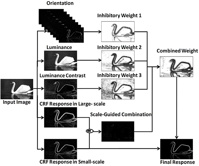
Figure 1. MCI framework revised from Yang et al. (2014).

Firstly, the response of one orientation-selective V1 neuron in CRF was calculated. For an input image I(x, y), the response e_i(x, y; θ_i, σ) was represented by the derivative of 2D Gaussian function correlated with preferred orientation θ_i and scale σ. After a winner - take - all strategy over N_θ different preferred orientations, the final CRF response E(x, y; σ) was calculated as in Equation (2),

$\begin{array}{ll}{\text{e}}_{\text{i}}\left(\text{x},\text{y};{\theta }_{\text{i}},\sigma \right)=\left|\text{I}\left(\text{x},\text{y}\right)\ast \frac{\partial \text{g}(\tilde{\text{x}},\tilde{\text{y}};{\theta }_{\text{i}},\sigma )}{\partial \tilde{\text{x}}}\right|& (1)\end{array}$

$\begin{array}{ll}\text{E}\left(\text{x},\text{y};\sigma \right)=\max \left\{{\text{e}}_{\text{i}}\left(\text{x},\text{y};{\theta }_{\text{i}},\sigma \right)|\text{i}=1,2,\dots ,{\text{N}}_{\theta }\right\}& (2)\end{array}$

Secondly, the local features were extracted, including orientation Θ (x, y), luminance L(x, y)and luminance contrast C(x, y). The computational equations of these features were shown in Equations (3) - (5), in which ω(x_i,y_i) was a raised cosine weighted window, S_xy represented the local square window, and $\mu =\sum _{({\text{x}}_{\text{i}},y_i)\in {\text{S}}_{\text{xy}}}\omega ({\text{x}}_{\text{i}},y_i)$.

$\begin{array}{ll}\Theta \left(\text{x},\text{y}\right)={\left[{\text{e}}_1,{\text{e}}_2,\dots ,e_{{\text{N}}_{\theta }}\right]}_{(\text{x},\text{y})}^{\text{T}}& (3)\end{array}$

$\begin{array}{ll}\text{L}\left(\text{x},\text{y}\right)=\frac{1}{\mu }{\displaystyle \sum _{\left({\text{x}}_{\text{i}},{\text{y}}_{\text{i}}\right)\in {\text{S}}_{\text{xy}}}\omega \left({\text{x}}_{\text{i}},{\text{y}}_{\text{i}}\right)\text{I}\left({\text{x}}_{\text{i}},{\text{y}}_{\text{i}}\right)}& (4)\end{array}$

$\begin{array}{ll}\text{C}\left(\text{x},\text{y}\right)=\sqrt{\frac{1}{\mu }{\displaystyle \sum _{\left({\text{x}}_{\text{i}},{\text{y}}_{\text{i}}\right)\in {\text{S}}_{\text{xy}}}\omega \left({\text{x}}_{\text{i}},{\text{y}}_{\text{i}}\right)\frac{{(\text{I}\left({\text{x}}_{\text{i}},{\text{y}}_{\text{i}}\right)-\text{L}\left(\text{x},\text{y}\right))}^2}{\text{L}{\left(\text{x},\text{y}\right)}^2}}}& (5)\end{array}$

Thirdly, the inhibitory weights W_{Θ(x, y)}, W_{L(x, y)}, W_{C(x, y)} were computed based on the center-surround mechanisms at each location for each feature, in which ${\stackrel{\overline{\Theta }}{}}_{\text{CRF}}$(x, y) was the orientation vector computed by Gaussian weighted averaging of Θ( x,y ) in the region of CRF. The distance - related weighting function was denoted as W_d, which meant that the strength of surround inhibition decreased with the increasing distance from the CRF center.

$\begin{array}{ll}{\text{W}}_{\Theta }\left(\text{x},\text{y}\right)=\exp \left(-\frac{{\Vert {{ }^{\overline{\Theta }}}_{\text{CRF}}(\text{x},\text{y}){-}^{\overline{\Theta }}{ }_{\text{NCRF}}(\text{x},\text{y})\Vert }^2}{2{\sigma }_{\Delta \theta }^2}\right)& (6)\end{array}$

$\begin{array}{ll}{\text{W}}_{\text{L}}\left(\text{x},\text{y}\right)={\displaystyle \sum _{({\text{x}}_{\text{i}},{\text{y}}_{\text{i}})}\exp \left(-\frac{\left|\text{L}\left(\text{x},\text{y}\right)-\text{L}({\text{x}}_{\text{i}},{\text{y}}_{\text{i}})\right|{}^2}{2{\sigma }_{\Delta l}^2}\right)}{\text{W}}_{\text{d}}\left({\text{x}}_{\text{i}}-\text{x},{\text{y}}_{\text{i}}-y\right)& (7)\end{array}$

$\begin{array}{ll}{\text{W}}_{\text{C}}\left(\text{x},\text{y}\right)={\displaystyle \sum _{({\text{x}}_{\text{i}},{\text{y}}_{\text{i}})}\exp \left(-\frac{{\left|\text{C}\left(\text{x},\text{y}\right)-\text{C}({\text{x}}_{\text{i}},{\text{y}}_{\text{i}})\right|}^2}{2{\sigma }_{\Delta \text{c}}^2}\right)}{\text{W}}_{\text{d}}\left({\text{x}}_{\text{i}}-\text{x},{\text{y}}_{\text{i}}-\text{y}\right)& (8)\end{array}$

Then, these three weights were integrated into a unified weight W_com based on a scale - guided combination strategy, where N(·) was a linear normalization operator.

$\begin{array}{l}{\text{W}}_{\text{com}}\left(\text{x},\text{y}\right)\\ =\{\begin{array}{l}\max \left({\text{W}}_{\Theta ,}{\text{W}}_{\text{L}},{\text{W}}_{\text{C}}\right)\left(\text{x},\text{y}\right),\text{N}\left(\text{E}\left(\text{x},\text{y};\sigma \right)\right)-\text{N}\left(\text{E}\left(\text{x},\text{y};2\sigma \right)\right)>0\\ \min \left({\text{W}}_{\Theta ,}{\text{W}}_{\text{L}},{\text{W}}_{\text{C}}\right)\left(\text{x},\text{y}\right),\text{N}\left(\text{E}\left(\text{x},\text{y};\sigma \right)\right)-\text{N}\left(\text{E}\left(\text{x},\text{y};2\sigma \right)\right)\le 0\end{array}& (9)\end{array}$

Finally, the final response Res(x, y) was calculated based on the final inhibitory weight.

$\begin{array}{l}\text{Res}\left(\text{x},\text{y}\right)=\text{H}(\text{E}\left(\text{x},\text{y};\sigma \right)-\alpha ·{\text{W}}_{\text{com}}\left(\text{x},\text{y}\right)·\text{E}\left(\text{x},\text{y};\sigma \right)\\ \ast {\text{W}}_{\text{d}}\left(\text{x},\text{y}\right))& (10)\end{array}$

$\begin{array}{ll}\text{where},\text{H}\left(\text{z}\right)=\{\begin{array}{c}0\text{z}<0\\ \text{z}\text{z}\ge 0\end{array}& (11)\end{array}$

Based on the above framework, MCI is applied to obtain the contours of natural images. Figure 2 gives some contour extracting results of MCI. Figure 2A represents input images, Figure 2B is final contour response without post-processing, Figure 2C represents the real-valued probability of contours after non-max suppression, Figure 2D is the binary image (containing values 0 or 1) after hysteresis thresholding. From the red box in Figure 2B, we can easily see that some texture contours obtained by the MCI do not belong to the real one. Table 1 shows the running time for every image in Figure 2, and the average time consuming of whole database (including 200 images for testing). And Table 1 also shows the runtime for every MCI step while the size of the input image is 481 × 321. It nearly takes 15 s to process an image, far from the processing speed of the human visual system. And the inhibitory weights at each location are computed for each feature, which consumes lots of time and does not compare to the fast and effective information processing in the human visual system. So, we propose an improved model, sMCI.

FIGURE 2

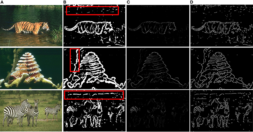
Figure 2. MCI results on natural images. (A) Input images. (B) Final contour responses without post-processing. The contour includes some unwanted textures located in red box. (C) Real-valued probability of contours after non-max suppression. (D) The binary images (containing values 0 or 1) after hysteresis thresholding.

TABLE 1

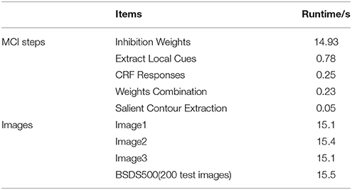
Table 1. The runtime of each step for MCI and the whole time on some images and the average time of BSDS 500.

The sMCI Model

Prior Filtering and Uniform Sampling

To accelerate MCI, we improved it from two facts, which are prior filtering and uniform sampling. We will first introduce the process of prior filtering.

As shown in Figure 3, the salient object is located in the red box, which occupies a small portion relative to the whole image. Meanwhile, the contours of the object are salient relative to the background. Therefore, based on these observations, we only select the pixels, with their response value above 30% of the largest response after filtered with Gabor, to speed up the calculation of the inhibitory weights. The computing process is as the following:

$\begin{array}{ll}{\text{W}}_{\Theta }\left(\text{x},\text{y}\right)=\{\begin{array}{ll}1\hfill & \text{Loc}\left(\text{x},\text{y}\right)=0\hfill \\ \exp \left(-\frac{{\Vert {{ }^{\overline{\Theta }}}_{\text{CRF}}(\text{x},\text{y}){-}^{\overline{\Theta }}{ }_{\text{NCRF}}(\text{x},\text{y})\Vert }^2}{2{\sigma }_{\Delta \theta }^2}\right)\hfill & \text{Loc}\left(\text{x},\text{y}\right)=1\hfill \end{array}& (12)\end{array}$

where $\text{Loc}\left(\text{x},\text{y}\right)=\{\begin{array}{c}0\text{ E}\left(\text{x},\text{y};\sigma \right)-30\%\ast {\text{E}}_{\max }<0\\ 1\text{ E}\left(\text{x},\text{y};\sigma \right)-30\%\ast {\text{E}}_{\max }\ge 0\end{array}$, in which E_max represents the largest one of the entire image CRF responses.

FIGURE 3

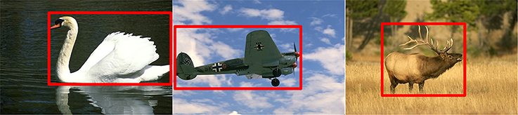
Figure 3. The mechanism of the prior filtering: most of the true contours are located in the red box, with low percentages in the whole image.

Another observation is that the characteristics of adjacent neurons response have strong correlations which suggests that their responses are similar (Kohn, 2005). Based on this fact, there is no need to calculate the inhibitory weights of all neurons for each input image. The inhibitory responses of all neurons can be approximated by those of partial neurons.

The other way to speed up the computation is sampling. This paper presents two sampling methods: sampling in one direction and in both directions. The detailed steps of two uniform sampling methods are as follows:

As shown in Figure 4, the black point in Figure 4A represents the location in the image. In the original MCI algorithm, the inhibitory weights are calculated at each location for every feature. For the uniform sampling in the x-direction, we just need to calculate the inhibitory weights of the black points in Figure 4B, and the inhibitory weights of the remaining points are obtained by the weighted sum of the nearby points. For example, the weight of the blue point can be obtained based on the two black points whose weights are known. Meanwhile, based on the biological mechanism that the influence of nearby neurons is greater than the one of distant neurons, the calculation formula of the inhibitory weights of the missing blue point in Figure 4B is in Equation (13):

$\begin{array}{ll}{\text{W}}_{{\text{p}}_1}=\frac{2}{3}\times {\text{W}}_{{\text{x}}_1}+\frac{1}{3}\times {\text{W}}_{{\text{x}}_2}& (13)\end{array}$

where W_p1 denotes the unknown weight of blue point, W_x1 and W_x2 represent the black points whose weights have been calculated. This also applies to the sampling in the y-direction.

FIGURE 4

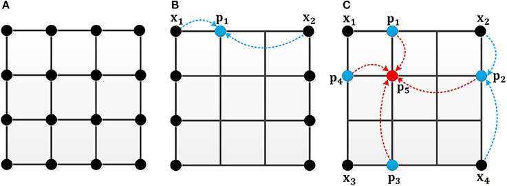
Figure 4. The mechanism of the uniform sampling. (A) The inhibitory weights at each location need to be calculated. (B) The uniform sampling in the x-direction. Only the weights at the black points need to be calculated. The blue points can be represented by the nearby black points. (C) The uniform sampling in x, y direction. The blue points can be calculated from the nearby black points. The red point can be obtained by the nearby blue points.

In Figure 4C, an illustration is given to clarify the sampling process in both x and y directions. For a 4 × 4 image, only the weights of four black points are computed. The weights of the blue points are computed by two black points, and the weight of the red point can be represented by the weights of the four blue points. The calculation of inhibition weights of the missing blue points in Figure 4C is given in Equation (14):

$\begin{array}{ll}{\text{W}}_{{\text{p}}_2}=\frac{2}{3}\times {\text{W}}_{{\text{x}}_2}+\frac{1}{3}\times {\text{W}}_{{\text{x}}_4}& (14)\end{array}$

and then the calculation of the weight of the missing red point is obtained by equation (15).

$\begin{array}{l}{\text{W}}_{{\text{p}}_5}=\frac{1}{3}\times {\text{W}}_{{\text{p}}_1}+\frac{1}{3}\times {\text{W}}_{{\text{p}}_4}+\frac{1}{6}\times {\text{W}}_{{\text{p}}_2}+\frac{1}{6}\times {\text{W}}_{{\text{p}}_3}\\ =\frac{4}{9}\times {\text{W}}_{{\text{x}}_1}+\frac{2}{9}\times {\text{W}}_{{\text{x}}_2}+\frac{2}{9}\times {\text{W}}_{{\text{x}}_3}+\frac{1}{9}\times {\text{W}}_{{\text{x}}_4}& (15)\end{array}$

Where W_x1, W_x2, W_x3 and W_x4 represent the black points whose weights are known, W_p1, W_p2, W_p3, and W_p4denote the unknown weights of blue points, W_p5 denotes the unknown weight of the red point.

Finally, the prior filtering and uniform sampling are combined to further accelerate the speed of the method. To avoid losing too much real contour information, the following fusion method is adopted: for an image, we first select the pixels with their values above 10% of the largest response after filtered with Gabor, and then sample these pixels uniformly to further shorten the running time and ensure the integrity of the contour information.

Sparse Coding

After accelerating the algorithm, we propose a method based on the biological mechanism to suppress the unwanted texture as shown in Figure 2.

Barlow (1981) has made a statistical and comprehensive analysis of the total number of cells in the visual pathway of macaques, which are shown in Table 2. The number of neurons in the lateral geniculate nucleus (LGN) is almost equal to the number of neurons in the ganglion, and the number of cells in the V1 region is much higher than that of the retina and the LGN. This comparison suggests that the responses of the V1 neurons have sparse properties. For the human visual system, sparse coding is crucial in encoding the input image, which can effectively suppress the redundant information. The local area containing some repeated textures will have a weak sparse response and the region including a stable boundary usually has a strong sparse response. Therefore, some unwanted contour noises can be effectively excluded based on the sparseness measure.

TABLE 2

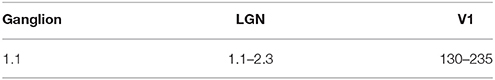
Table 2. Statistical data in the visual pathway of macaques (Unit: million) (Barlow, 1981).

In this paper, we compute the sparseness measure as mentioned in Kai-Fu Yang et al. (2015) and Hoyer (2004) to distinguish the texture region and the non-texture region. The formula is as follows

$\begin{array}{ll}\text{sparseness}\left(\text{x},\text{y};\overrightarrow{\text{h}}\right)=\frac{1}{\sqrt{\text{n}}-1}\left(\sqrt{\text{n}}-\frac{{\Vert \overrightarrow{\text{h}}\left(\text{x},\text{y}\right)\Vert }_1}{{\Vert \overrightarrow{\text{h}}\left(\text{x},\text{y}\right)\Vert }_2}\right)& (16)\end{array}$

where $\vec{\text{h}}(\text{x},\text{y})$ denotes the gradient's magnitude histogram of a local region centered at (x, y), n denotes the dimensionality of $\vec{\text{h}}(\text{x},\text{ y})$, and $\left|\right|\vec{\text{h}}(\text{x},\text{ y})|{|}_{\text{p}}$ denotes the l_p of $\vec{\text{h}}(\text{x},\text{ y})$, such as $\left|\right|\vec{\text{h}}(\text{x},\text{ y})|{|}_1=\sum |{\text{h}}_{\text{i}}|$, $\left|\right|\vec{\text{h}}(\text{x},\text{ y})|{|}_2=\sqrt{\sum |{\text{h}}_{\text{i}}{|}^2}$.

Then, the final neuron response FinalRes can be obtained by combining the original response Res and the sparseness, which is calculated as follows:

$\begin{array}{ll}\text{FinalRes}=\text{Res}\cdot \text{sparseness}\left(\text{x},\text{y};\overrightarrow{\text{h}}\right)& (17)\end{array}$

Experiments and Results

To evaluate the effectiveness of the proposed model, we test it on the BSDS500. The quantitative performance is compared with the original MCI model.

Experiment Settings

We test our model on the Berkeley Segmentation Data Set (BSDS500) (Martin et al., 2001). The BSDS500 is a dataset provided by the Berkeley computer vision group for image segmentation or contour detection, which includes 200 training, 200 testing, and 100 validation images. Boundaries in each image are labeled by several workers and are averaged to form the ground truth.

The performance is evaluated by the F-score (Martin et al., 2004), which denotes the similarity of the detected contours between human subjects and the algorithms. It is defined as F-score = 2PR / (P + R), where P represents the precision, R represents the recall.

Table 3 summarizes the meanings of the parameters involved in models, for example, the factor α in equation 10 denotes the connection strength between the CRF and the non-CRF. The parameter settings adopted in the MCI and sMCI model are the same.

TABLE 3

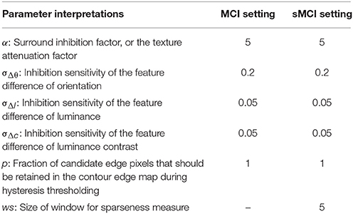
Table 3. Parameter interpretations and settings (Yang et al., 2014).

Results of Prior Filtering and Uniform Sampling

The prior filtering adopts 30% of the largest responses as the threshold, whereas prior filtering in combined method adopts 10% of the largest responses. We compare the results of prior filtering, uniform sampling and the combined one with the original MCI algorithm and the results are shown in Figure 5. The F-score results and the running time are shown in Table 4. From these results, we can find that running time of the prior filtering method is relatively short but gets a lower F-score value. We amplify patch in the green box of Figure 6A and show it in Figures 6B–E. We can clearly see that some contours in red box extracted by prior filtering are lost depicted in Figure 6B. However, contours extracted by uniform sampling methods are complete, shown in Figures 6C,D. The running time is nearly the same if only sampling in one direction, and the same for the accuracy. However, the performance of uniform sampling in one direction outperforms sampling in both x and y directions, although the latter is superior to the former in running time. So, the combined method adopts sampling in one direction. And the result shows that the combined method can shorten the running time and keep the performance.

FIGURE 5

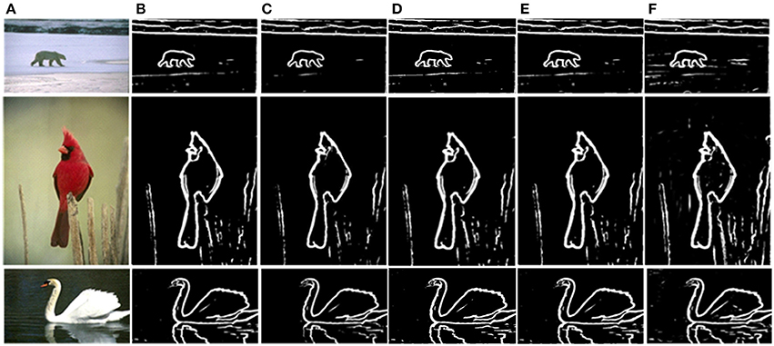
Figure 5. Comparison of experimental results. (A) Input images. (B) MCI results. (C) Prior filtering results. (D) Uniform sampling in the x-direction. (E) Uniform sampling in x, y direction. (F) Combined method.

TABLE 4

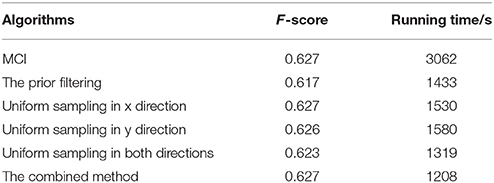
Table 4. Evaluation results and the runtime on BSDS 500 of the original MCI algorithm, the prior filtering, the uniform sampling in the x-direction, the uniform sampling in the y-direction, the uniform sampling in both directions, the combined method.

FIGURE 6

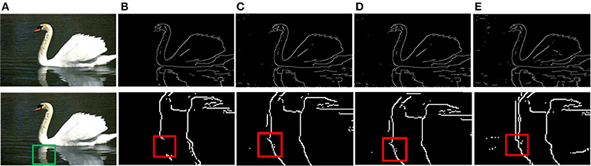
Figure 6. Results of three methods. (A) Input images. (B) Contour results after prior filtering with 30% largest responses. (C) Contour results after uniform sampling in the x-direction. (D) Contour results after uniform sampling in x, y direction. (E) Contour results after combined method.

Results of Sparse Coding and Final Evaluation

Although the above method can solve the problem of time-consuming effectively, there are still unnecessary contour noises in sMCI results. Therefore, we use the sparse coding to suppress the unwanted edges. The experimental results of sparseness are shown in Figure 7, including the whole contour results and details. As shown in Figure 7B, the textures on tiger's tail are unwanted edges, and the sparse response is weak at that location illustrated in Figure 7C. By the process of sparse coding, the unwanted texture at the tail is suppressed shown in Figure 7D.

FIGURE 7

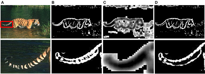
Figure 7. Results after sparse coding. (A) Input images. (B) Responses of the sMCI before sparse coding. (C) Sparseness responses. (D) Final responses after sparse coding.

The final results after non-maxima suppression (Canny, 1986) between MCI and sMCI models are shown in Figure 8. Figure 8A is the original image, Figure 8B represents the ground truth, Figure 8C is the MCI result and Figure 8D is the sMCI result. The F-score values are shown in Table 5.

FIGURE 8

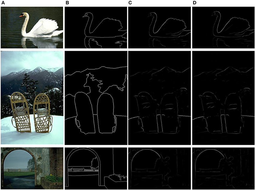
Figure 8. Evaluation images and results by MCI and sMCI. (A) Input images. (B) Ground truth. (C) MCI results (F-score = 0.627). (D) sMCI results (F-score = 0.629).

TABLE 5

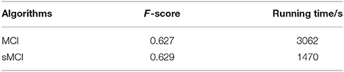
Table 5. Evaluation results for MCI and sMCI after sparse coding.

The experimental results demonstrate that sMCI model effectively reduces the running time by 52% without degrading the performance in contour accuracy.

Discussion

Based on the MCI algorithm, we proposed a fast contour detection model, inspired by the information processing mechanism in the human primary vision system. The prior filtering and uniform sampling effectively reduced the running time. And the sparse coding served to exclude the unwanted textures. The results on BSDS500 showed the competitive performance and fastness of the model.

The bright spots of our work can be summarized below. (a) We adopt the prior filtering based on the knowledge of human behavioral psychology, which can focus on the area containing the desired contours. (b) Uniform sampling is introduced based on the biological mechanism that nearby neurons often have highly correlated responses and thus include redundant information. We only calculate the weights of the partial feature rather than the whole images and reconstructs the whole feature responses based on properties between nearby neurons. (c) Sparse coding is introduced in the model, which provided an effective way to suppress the unwanted edges. The experimental results showed that the method can decrease the running time as well as keeping the accuracy of the contour detection.

However, the mechanism of the algorithm still has a gap with the human visual system. Therefore, how to optimize the model based on more biological mechanisms is our next step.

From the bottom-up mechanism, we can integrate more underlying features. In our work, we only consider features such as the orientation, the luminance, and the luminance contrast. However, the color contrast is also a crucial feature for contour detection. And in the human visual system, the color information is modulated by color-opponent mechanisms. One important extension of our current model is how to utilize the cue of color in an effective way. In future, we can design a framework combining the center-surround and color-opponent mechanisms to optimize the performance of contour detection.

From the top-down mechanism, we can integrate the feedback mechanism which plays an important modulatory role to the V1 neurons' responses. In fact, it is very challenging to extract the salient object boundaries in complex environments. And a feedback process can provide attentional support to salient or behaviorally-relevant features.

In summary, the model we proposed based on the biological mechanisms in this paper can both keep the accuracy and decrease the time-consuming. In the study, we can find that the neuroscience research promotes the development of the model research. In the future, the current research will be extended with more neuroscience results. From these studies, we also hope to understand the inner mechanisms of the information processing of the human brain.

Author Contributions

XK, QK, and YZ designed the work. XK and QK contributed to the experiments. XK, QK, YZ, and BX contributed to the results analysis. XK, QK, YZ, and BX contributed to the writing of the manuscript. The version of work is approved to be published by BX, YZ, QK, and XK.

Funding

This work was supported by the National Natural Science Foundation of China (61403375) and the CETC Joint Fund under Grant No.6141B08010103.

Conflict of Interest Statement

The authors declare that the research was conducted in the absence of any commercial or financial relationships that could be construed as a potential conflict of interest.

References

Allman, J., Miezin, F., and McGuinness, E. (1985). Stimulus specific responses from beyond the classical receptive field: neurophysiological mechanisms for local-global comparisons in visual neurons. Annu. Rev. Neurosci. 8, 407–430. doi: 10.1146/annurev.ne.08.030185.002203

PubMed Abstract | CrossRef Full Text | Google Scholar

Barlow, H. B. (1981). The Ferrier Lecture, 1980. Critical limiting factors in the design of the eye and visual cortex. Proc. R. Soc. London. Ser. B Biol. Sci. 212, 1–34. doi: 10.1098/rspb.1981.0022

PubMed Abstract | CrossRef Full Text | Google Scholar

Canny, J. (1986). A computational approach to edge detection. IEEE Trans. Pattern Anal. Mach. Intell. 8, 679–698. doi: 10.1109/TPAMI.1986.4767851

PubMed Abstract | CrossRef Full Text

Caselles, V., Kimmel, R., and Sapiro, G. (1997). Geodesic active contours. Int. J. Comput. Vis. 22, 61–79. doi: 10.1023/A:1007979827043

CrossRef Full Text | Google Scholar

Fitzpatrick, D. (2000). Seeing beyond the receptive field in primary visual cortex. Curr. Opin. Neurobiol. 10, 438–443. doi: 10.1016/S0959-4388(00)00113-6

PubMed Abstract | CrossRef Full Text | Google Scholar

Grigorescu, C., Petkov, N., and Westenberg, M. A. (2003). Contour detection based on nonclassical receptive field inhibition. IEEE Trans. Image Process 12, 729–739. doi: 10.1109/TIP.2003.814250

PubMed Abstract | CrossRef Full Text | Google Scholar

Hoyer, P. O. (2004). Non-negative matrix factorization with sparseness constraints. J. Mach. Learn. Res. 5, 1457–1469.

Google Scholar

Hubel, D. H., and Wiesel, T. N. (1959). Receptive fields of single neurones in the cat's striate cortex. J. Physiol. 148, 574–591.

PubMed Abstract | Google Scholar

Jones, H. E., Grieve, K. L., Wang, W., and Sillito, M. (2001). Surround suppression in primate V1. J. Neurophysiol. 86, 2011–2028. doi: 10.1152/jn.2001.86.4.2011

PubMed Abstract | CrossRef Full Text | Google Scholar

Kohn, A. (2005). Stimulus dependence of neuronal correlation in primary visual cortex of the macaque. J. Neurosci. 25, 3661–3673. doi: 10.1523/JNEUROSCI.5106-04.2005

PubMed Abstract | CrossRef Full Text | Google Scholar

Konishi, S., Yuille, A. L., Coughlan, J. M., and Zhu, S. C. (2003). Statistical edge detection: learning and evaluating edge cues. IEEE Trans. Pattern Anal. Mach. Intell. 25, 57–74. doi: 10.1109/TPAMI.2003.1159946

CrossRef Full Text | Google Scholar

La Cara, G. E., and Ursino, M. (2008). A model of contour extraction including multiple scales, flexible inhibition and attention. Neural Netw. 21, 759–773. doi: 10.1016/j.neunet.2007.11.003

PubMed Abstract | CrossRef Full Text | Google Scholar

Li, Z. (1998). A neural model of contour integration in the primary visual cortex. Neural Comput. 10, 903–940. doi: 10.1162/089976698300017557

PubMed Abstract | CrossRef Full Text | Google Scholar

Long, L., and Li, Y. (2008). “Contour detection based on the property of orientation selective inhibition of non-classical receptive field,” in 2008 IEEE Conference on Cybernetics and Intelligent Systems (Chengdu), 1002–1006. doi: 10.1109/ICCIS.2008.4670920

CrossRef Full Text | Google Scholar

Maire, M., Arbeláez, P., Fowlkes, C., and Malik, J. (2008). “Using contours to detect and localize junctions in natural images,” in 26th IEEE Conference on Computer Vision and Pattern Recognition, CVPR (Anchorage, AK), 1–8. doi: 10.1109/cvpr.2008.4587420

CrossRef Full Text | Google Scholar

Martin, D., Fowlkes, C., Tal, D., and Malik, J. (2001). A database of human segmented natural images and its application to evaluating segmentation algorithms and measuring ecological statistics. Proc. IEEE Int. Conf. Comput. Vis. 2, 416–423. doi: 10.1109/ICCV.2001.937655

CrossRef Full Text | Google Scholar

Martin, D. R., Fowlkes, C. C., and Malik, J. (2004). Learning to detect natural image boundaries using local brightness, color, and texture cues. IEEE Trans. Pattern Anal. Mach. Intell. 26, 530–549. doi: 10.1109/TPAMI.2004.1273918

PubMed Abstract | CrossRef Full Text | Google Scholar

Papari, G., Campisi, P., Petkov, N., and Neri, A. (2007). A biologically motivated multiresolution approach to contour detection. EURASIP J. Adv. Signal Process. 2007:071828. doi: 10.1155/2007/71828

CrossRef Full Text | Google Scholar

Petkov, N., and Westenberg, M. A. (2003). Suppression of contour perception by band-limited noise and its relation to nonclassical receptive field inhibition. Biol. Cybern. 88, 236–246. doi: 10.1007/s00422-002-0378-2

PubMed Abstract | CrossRef Full Text | Google Scholar

Ren, X. (2008). “Multi-scale improves boundary detection in natural images,” in European Conference on Computer Vision, eds D. Forsyth, P. Torr, and A. Zisserman (Berlin; Heidelberg: Springer), 533–545. doi: 10.1007/978-3-540-88690-7_40

CrossRef Full Text | Google Scholar

Rosenfeld, A., Hummel, R., and Zucker, S. W. (1976). Scene Labeling by Relaxation Operations. IEEE Trans. Syst. Man. Cybern. 6, 420–433. doi: 10.1109/TSMC.1976.4309519

CrossRef Full Text | Google Scholar

Shen, Z.-M., Xu, W.-F., and Li, C.-Y. (2007). Cue-invariant detection of centre-surround discontinuity by V1 neurons in awake macaque monkey. J. Physiol. 583, 581–592. doi: 10.1113/jphysiol.2007.130294

PubMed Abstract | CrossRef Full Text | Google Scholar

Tang, Q., Sang, N., and Zhang, T. (2007a). Contour detection based on contextual influences. Image Vis. Comput. 25, 1282–1290. doi: 10.1016/j.imavis.2006.08.007

CrossRef Full Text | Google Scholar

Tang, Q., Sang, N., and Zhang, T. (2007b). Extraction of salient contours from cluttered scenes. Pattern Recognit. 40, 3100–3109. doi: 10.1016/j.patcog.2007.02.009

CrossRef Full Text | Google Scholar

Ursino, M., and La Cara, G. E. (2004). A model of contextual interactions and contour detection in primary visual cortex. Neural Netw. 17, 719–735. doi: 10.1016/j.neunet.2004.03.007

PubMed Abstract | CrossRef Full Text | Google Scholar

Yang, K.-F., Gao, S.-B., Guo, C.-F., Li, C. -Y., and Li, Y.-J. (2015). Boundary detection using double-opponency and spatial sparseness constraint. IEEE Trans. Image Process. 24, 2565–2578. doi: 10.1109/TIP.2015.2425538

CrossRef Full Text | Google Scholar

Yang, K., Gao, S., Li, C., and Li, Y. (2013). “Efficient color boundary detection with color-opponent mechanisms,” in Proceedings of the IEEE Computer Society Conference on Computer Vision and Pattern Recognition (Portland, OR), 2810–2817. doi: 10.1109/cvpr.2013.362

CrossRef Full Text | Google Scholar

Yang, K. F., Li, C.-Y., and Li, Y. (2014). Multifeature-based surround inhibition improves contour detection in natural images. IEEE Trans. Image Process. 23, 5020–5032. doi: 10.1109/TIP.2014.2361210

PubMed Abstract | CrossRef Full Text | Google Scholar

Zeng, C., Li, Y., and Li, C. (2011). Center-surround interaction with adaptive inhibition: a computational model for contour detection. Neuroimage 55, 49–66. doi: 10.1016/j.neuroimage.2010.11.067

PubMed Abstract | CrossRef Full Text | Google Scholar