Improved Understanding of Industrial Process Relationships Through Conditional Path Modelling With Process PLS

Introduction

Industrial (bio)chemical processes need to be monitored and controlled well to guarantee sustainable and high-quality production despite variations in external factors such as raw materials, weather, plant operators, equipment maintenance and customer wishes. A deep understanding of how the production plant operates under and responds to these conditions is crucial for the development of accurate process monitoring and control strategies. To considerable extent, such understanding follows from first-principle knowledge. In practice, however, influences of external factors on the production, daily operation of the plant cannot be described completely by these first principles. Multivariate statistical analysis of historical production data can therefore reveal an augmented insight into the process, as this data does reflect the daily and real operation rather than the engineered operation.

Examples of statistical modelling methods that are widely used for this purpose are Principal Component Analysis (PCA), Partial Least Squares (PLS), Support Vector Machines (SVM) and Artificial Neural Networks (ANN) (MacGregor & Kourti, 1995; Qin, 1997; Kourti, 2005; Cuentas et al., 2017). These methods are often employed for process fault diagnosis through multivariate control (Shewhart) charts and for predicting difficult-to-measure production indicators, such as product quality, from easy-to-measure process variables (soft-sensoring) (Bersimis et al., 2007; Kadlec et al., 2009). Though these methods can be used to quantify the relationships between individual process parameters and variables, they provide limited higher-level insight into the relationships between different production units, as limited higher-level structural knowledge about the plant is employed.

The use of path analysis or structural equation modelling methods to industrial data analysis is therefore becoming increasingly popular, as these methods explicitly model the valuable information about relationships and can be considered explainable artificial intelligence (Höskuldsson et al., 2007; Gade et al., 2019). In general, path analysis methods estimate the directional statistical relationship between groups of measured variables. For industrial data, grouping process variables by the production unit in which they are measured thus allows for the estimation of how much operations of different production units are mutually related. This incorporates the physical structure of the production plant in the analysis of the data, of which the results in turn can be interpreted in the context of that structure (van Kollenburg G. H. et al., 2020).

Different methods for path analysis exist, including PLS-path modeling (Hair et al., 2011), sequential and orthogonalized PLS-path modeling (Romano et al., 2019), sequential multi-block PLS (Lauzon-Gauthier et al., 2018), multiblock kernel PLS (Zhang et al., 2010) and network PCA (Codesido et al., 2020). PLS-PM in particular is a well-established method in social sciences, but its high value for modelling industrial production data is also already demonstrated (van Kollenburg G. H. et al., 2020). Another path analysis method that has been developed very recently, is Process PLS (van Kollenburg et al., 2021). This method improves upon the mathematical limitations of PLS-PM and is better suited to model the complexity and heterogeneity of industrial production data as a network.

Process PLS is more appropriate for path modelling industrial data than alternative methods for three main reasons. Firstly, it can model multiple latent variables per group of process variables, in contrast to for instance PLS-path modeling. It can thus describe multiple sub-processes per production step, which are present for most industrial processes. Secondly, it can cope with the multicollinearity that the process variables of production steps often show (Guo et al., 2019). This gives rise to a more accurate estimation and better interpretability of the relationships between the production steps. Lastly, Process PLS (like PLS-path modeling but unlike for instance sequential and orthogonalized PLS-path modeling) does not require any a priori (importance) ranking to be imposed on the production steps, which in practice is difficult to do even for process experts (van Kollenburg et al., 2021a).

The relationships estimated with path modeling give much insight into the structure of the plant. Their sizes may even be related to an external production factor that is not directly included in the model, such as production cost (van Kollenburg G. H. et al., 2020). An even more exhaustive understanding of a plant’s behavior can however be obtained by quantifying how the process relationships are affected by multiple, possibly interacting operating conditions, such as production season, year, parallel lines or product quality ranges. Such an analysis yields an elaborate insight into how the plant’s operation is different under different combinations of production conditions. This allows process operators and engineers to even better steer the plant to cope with production variations caused by those multilevel conditions.

This paper presents a systematic approach for performing such a conditional path analysis on historical production data, using Process PLS. The work focuses on the use of Process PLS for such modelling, and a comparison to conditional modelling using alternative path modelling methods is out of scope for the current work. A large dataset from an industrial-scaled milk protein powder production plant is separated based on one or more operating conditions, after which each data subset is modelled and quantitatively compared. A thorough discussion of how the results of the analysis can be visualized, interpreted and communicated with and among process operators and engineers is provided.

Methods and Data

Process PLS

A Process PLS model comprises two user-defined parts: the inner (structural) and outer (measurement) model. A production plant’s structure can be modelled by grouping of the process variables ($X$) in the outer model according to the production units (or production steps). A group of variables is then called a block. The inner model defines which directional relationships are estimated between which production steps. For each unit, one or more latent variables ($LV$) are constructed to represent the major sources of covariance between the process variables of blocks which are connected in the inner model. The contribution of a process variable to specific latent variables for that unit are called weights ($R$, in some literature also referred to as $W$). Effects of the latent variable on other latent variable in the inner model are represented as explained variances (${\text{Ρ}}^2$, i.e. ‘rho-squared’). The design of a Process PLS model is similar to that of a PLS-PM model, and is visualized in Figure 1 for an example process. The relationships in the inner model may represent for instance a direct physical connection (piping), indirect connection between similar variables being measured at different locations), or feedforward control loops. As only recursive (non-cyclic) pathways can be modelled, feedbacks of either (intermediate) product or operation control actions cannot be directly modelled, but the process set points of a control scheme and/or the level of (intermediate) product feedback may for instance be used as a variable in the Process PLS outer model.

FIGURE 1

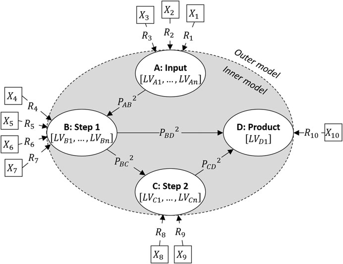
FIGURE 1. The design of a Process PLS model for an example two-step production process. The input and product are also modelled as steps in order to estimate their relationships to the two production steps.

Estimation of a Process PLS model is done by iteratively optimizing a network of PLS-models using the SIMPLS-algorithm (de Jong, 1993). First, the dimensionality of the blocks is reduced to obtain estimates for the latent variables which maximize the covariance between interconnected blocks through a set of PLS2 regressions, one for each block of variables. To estimate the latent variables of a given step with PLS2, the process variables of that step are used as predictors and the process variables of all steps that step has a relationship to are used as responses. Only when a step has only incoming relationships, the process variables of the steps that have a relationship to that step are used as predictors and the process variables of the step itself are used as responses. The number of latent variables per block can be manually fixed if desired or optimized by internal cross-validation (which is the default in the software implementation used for the results in this paper, see Software). The process variable weights ($R$) are effectively the contributions of the variables to the relationships modelled by these PLS models. After the latent variables are estimated, a second set of PLS regressions is performed to estimate the relations in the inner model. The strengths of these relationships ($P^2$) are calculated from the PLS2 regression coefficients and represent the fraction of variance that the latent variables in a predictor block can explain in the response block. As Process PLS does not take into account process dynamics like mechanistic modelling approaches, knowledge about the kinetics of the process are not required for modelling. More details on the Process PLS method may be found in (van Kollenburg et al., 2021a).

Demonstrator Process

The industrial production facility investigated is a well-controlled plant that produces milk protein powder from skim milk. The skim milk is heated, after which it is subjected to two precipitation steps. The resulting curd is washed, dissolved in an alkali solution, and finally dried to a powder. The critical product quality indicator for the protein powder is the mineral content, which should be as low as possible. More details on milk powder production can be found in the dairy processing handbook (Bylund, 1995).

Data Collection

The data used in this study corresponds to three parallel production lines and three consecutive production years, and was not originally collected for other purposes than the current study. The data comprises 51 process variables, which are the same for the different production lines and are distributed across the processing steps as given in Table 1. All variables represent physical measurements, and not setpoints or production status values. Only data from effective production time was used in the current analysis. The variable representing the product quality is the mineral content mentioned earlier, which is measured at-line at a relatively low frequency (hourly basis). The variable on incoming milk is also measured at similar frequency. All other variables are process variables such as temperatures, pressures and flow rates, and are measured in- or on-line at high frequency. The specific identities of these variables will not be disclosed as they are not relevant for the conclusions in this paper.

TABLE 1

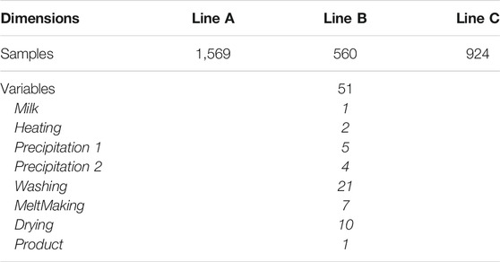
TABLE 1. Number of samples and variables of the data collected for each of the three production lines, after synchronization and cleaning as explained in Data preparation.

Data Preparation

Because the process variables are measured at separate locations and at different time intervals, the collected data had to be synchronized to obtain a multivariate dataset that can readily be analyzed. The high-frequency process variables were synchronized to the low-frequency product quality variable using median-filtering with a 3 h wide window, systematically selected as optimal synchronization (Offermans et al., 2020). This method also allows for a small degree of process dynamics to be included in the modelling procedure, as each synchronized sample represents the measurements done in the 3 hours before its sampling time. Time-lags between individual process variables are not taken into account. For the relative low-frequency measurements on incoming milk, the most recent measured value was matched to each mineral content sample. Missing values can be and were present after the synchronization procedure, and were imputed by replacing them by the median of the values that were present (Souza et al., 2016). This was done per production line and per production variable. Outlying samples were detected per production line using the multivariate Hotelling’s $T^2$- and $Q$-statistics calculated from PCA models explaining at least 70% variance of the autoscaled data. Samples for which at least one statistic was over three standard deviations removed from the median were removed (Varmuza and Filzmoser, 2016). The number of samples obtained after the data collection, synchronization and cleaning are given in Table 1.

Path Modelling Conditional to Single Operation Conditions

The first part of the study focused on investigating the effects of the individual production conditions separately on the process relationships. The three (multilevel) conditions that were explored are production line, production season and product quality. All data was for instance only separated according to the three production lines. For separating the data into seasons, meteorological seasons were used as these are identical for each year. The mineral content values were used to separate the data into three relative product quality ranges. The boundaries of these ranges were set at the 1^st and 2^nd tertiles to ensure comparable sample sizes for all models, as is illustrated in Figure 2. As mentioned before, a low mineral content value indicates a high-quality production.

FIGURE 2

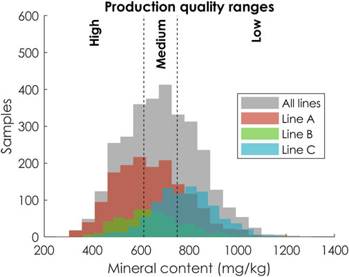
FIGURE 2. Ranges for the product mineral content measurements used to separate the data based on product quality.

Each data subset was individually modelled with Process PLS, using the same inner and outer model specification for each model. The directional relationships between the production steps that were estimated using Process PLS are illustrated in Figure 3. The inner model, shown in Figure 3, was specified according to two criteria introduced by van Kollenburg et al. (van Kollenburg G. H. et al., 2020). Firstly, relationships of each step on the subsequent step are included (counter-clockwise, starting from the top, in Figure 3). These represent the physical architecture of the plant and the flow of the process (piping). Secondly, direct relationships of each production step on the product-variables and thus the product quality are included. The outer model, which relates the process variables to the different production steps, was specified based on the physical location of each process variables. The number of variables per step thus are reported in Table 1.

FIGURE 3

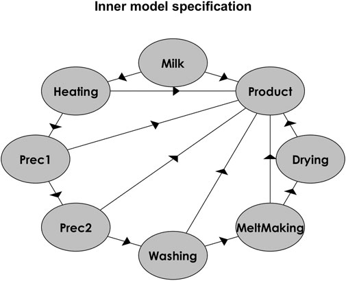
FIGURE 3. Inner model specification used for path modelling of the milk protein powder production process.

The number of latent variables considered for each block/step was optimized using the default cross-validation procedure in the Process PLS implementation used (‘pathmodelr’). Before modelling, all individual process variables were autoscaled to have zero mean and unit standard deviation, after which the process variables are collectively but per step rescaled so that each step has a sum of squares of 1. This is the default procedure by pathmodelr. All remaining modelling settings were also kept at their default values. To estimate the precision of the modelled process relationships, each Process PLS model was subjected to a non-parametric bootstrap with 200 replicates (Johnson, 2001).

Path Modelling on Multiple Production Conditions

For the second part of the study, the full data was separated on all production conditions at once, following a full factorial design. Each data subset was modelled using Process PLS, to calculate the process relationships for each possible combination of production conditions. Three-way ANOVA analyses were used to estimate the main and interaction effects of the production conditions on each separate process relationship and process variable weight (Huitson et al., 1976). This allows for the investigation of interactions between the production conditions on the process relationships, for instance between production season and line. The boundaries for the quality ranges were, as before, set relatively at the 1^st and 2^nd tertiles. They were set per combination of line and season, to ensure sufficient samples in each experiment for reliable modelling. The design matrices for the experimental design and the sample sizes for each experiment (and thus Process PLS model) are shown in Supplementary Table S1 in the supplemental material.

The modelling and bootstrapping procedure for each data subset (full factorial design experiment) was identical to that used before while investigating the separate production conditions. The three-way ANOVA analyses were performed on the mean results found after bootstrapping. A False Discovery Rate (FDR) correction was applied to the $p$-values obtained with ANOVA using the method proposed by Benjamini and Hochberg to adjust for multiple testing errors (Benjamini and Hochberg, 1995). This because the relationships and dependencies identified with the proposed analysis may require further investigation by plant personnel, which is time and cost intensive. As such, false positives (type I) errors are more harmful and less desirable than false negatives (type II) errors.

A schematic overview of the different data preparation, separation, modelling and interpretation steps performed as part of the presented study on conditional path modelling is shown in Figure 4.

FIGURE 4

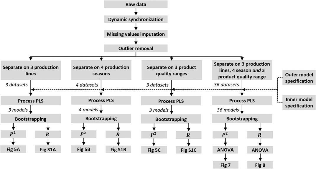
FIGURE 4. Schematic overview of the conditional path modelling analyses presented.

Software

Data preparation was done using MATLAB R2017a (MATLAB, 2017). Modelling data with Process PLS was done in R, using the pathmodelr package version 0.1.2 (Team R Development Core, 2018; van Kollenburg G. H. et al., 2020).

Results and Discussion

Path Modelling Conditional to Single Operation Conditions

Figures 5A–C show the primary modelling results found after partitioning the complete data only on either production line, production season or product quality range (respectively). Shown are the proportions of variance explained ($P^2$) for each relationship in the inner model (as shown in Figure 3). These values quantify the directional relationship between the production steps. Shown per relationship are the mean values over the 200 bootstrapping replicates. The 99% confidence intervals are plotted as error whiskers but are for many results too small to discern. This indicates that the results have high precision and attests that Process PLS is a robust method for statistical modelling of industrial data.

FIGURE 5

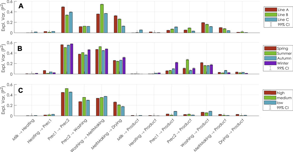
FIGURE 5. (A–C): Size of process relationships in terms of fractions of explained variance (P²), as found when using Process PLS modelling on either separate production lines (A), or production season (B), or product quality range (C). The bars represent the means and the whiskers represent the 99% confidence intervals over 200 bootstrap replicates.

The results in Figures 5A,B give insights into the relationships within the process, and how they differ under various production conditions. Firstly, they show which relationships are overall strongest. For this process, the relationship from Prec1 to Prec2 is in general the strongest, irrespective of production line, season, or product quality range. These steps are likely strongly related because they have a similar function in the process. From all the production steps, Washing relates strongest to Product under most conditions. This indicates that Washing may be the most influential step for the product quality, and future optimization efforts should be directed to this step. Importantly, Milk in general only relates to Product. Though this may sound counter-intuitive, it indicates that variations in Milk do not influence the production quality. In turn, this supports the notion that the process is well-controlled and that stable production quality is achieved despite raw material variations.

Results from the conditional modelling show that the relationship between Prec1 and Prec2 is weaker for production line B than for the other production lines (Figure 5A). This indicates that the operation of Prec2 is less related to that of Prec1 in line B than in the other lines. Additionally, the relationship between Prec2 and Product is stronger for line B than for the other lines, indicating that variations in Prec2 are related to variations in Product. In a production process with a focus on constant quality, this results may be an important focus for follow-up investigations.

Separating the data only on production season (Figure 5B) reveals that the Prec1 relates stronger to Product in the winter, while Prec2 relates stronger to Product in the summer. This indicates that the focus of process control is different for the seasons, for instance because seasonal variation manifested in the raw material or weather influences the Prec1 and Prec2 steps differently. This is supported by Prec1 → Prec2 being lower in summer and higher in winter.

When looking at the different product quality ranges (Figure 5C), it is interesting that Washing → MeltMaking increases and MeltMaking → Drying decreases with decreasing product quality. This suggests that higher quality product is obtained when the operation of MeltMaking is more aligned with that of Drying (the step after it) than with that of Washing (the step before it). This should be further investigated, as it could indicate that aligning the MeltMaking settings with that of Drying instead of Washing leads to structurally higher production quality.

The results in Figures 5A–C give already much insight into the process but understanding of the process can be augmented by evaluating the weights ($R$) of the process variables in the Process PLS models. As an example, Figure 6 shows the weights for the variables corresponding to Prec1 and Prec2 in the models obtained after separating the data on production line alone. These weights represent the contributions of the process variables on the latent variables of their respective block. As previously discussed, the relationship between Prec1 to Prec2 is weaker for line B than for lines A and C (Figure 5A). Because Prec2 V2 has a particular high weight in the model of line B, plant operators and engineers could be advised to investigate the operation of this variable further. It likely has a characteristic behavior unique in line B that causes the operation of Prec2 to be less related to Prec1 which, as discussed earlier, may influence the product quality.

FIGURE 6

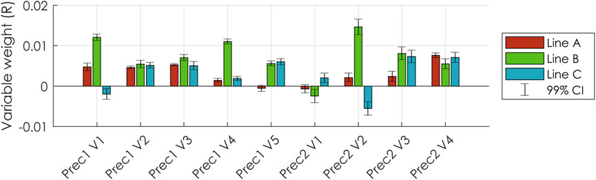
FIGURE 6. Weights (R) of the process variables of Prec1 and Prec2 in the different Process PLS models trained per production line. The bars represent the means and the whiskers represent the 99% confidence intervals over 200 bootstrap replicates.

This example illustrates how variable weights should be interpreted, and how investigating these may aid process operators and engineers in optimizing monitoring and control of a production plant. The variable weights can provide much more information, but discussing all of them for the process in this paper is of limited value, as their identities are disclosed. The weights of all variables for all models are given in the supplementary materials in Supplementary Figures S1A–C for the interested reader but are not discussed further here.

Path Modelling Conditional to Multiple Operation Conditions

Figure 7 displays the results of analyzing each combination of the three production conditions according to a full-factorial experimental design with the same Process PLS model and analyzing variations in the model parameters using an ANOVA. Note that this experimental design is applied to data that is already measured, and that is no further measurements are collected according to that design. As many PLS regressions are calculated during this experiment, 936.000 to be exact (36 production condition combinations, 13 inner relationships, 10 cross-validation repeats and 200 bootstrap repeats), it should be noted that the computation time for obtaining the results as presented in this manuscript is around 18 min when using a desktop computer with an Intel Core i7-7900 K processor. Although significant, this computation time should not be limiting for the use of the proposed methodology as a tool for off-line exploration of historical data. The number of cross-validation repeats and/or bootstrap repeats could be reduced to save computation time on slower systems, but the robustness of the models should be checked with additional care.

FIGURE 7

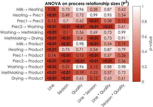
FIGURE 7. FDR-corrected$p$-values obtained by performing three-way ANOVA on the fractions of explained variance (P²) found with Process PLS according to the full factorial conditional path modelling approach. A low$p$-value signifies a low probability that the process relationship size is comparable under different (combinations of) production conditions.

Shown in Figure 7 are the FDR-corrected $p$-values of each three-way ANOVA that was performed per modelled process relationship size (in terms of mean explained variance, $P^2$, over bootstrap replicates). These results thus represent the inner path model. The $p$-values quantify the probability of the relationships sizes being identical regardless of a certain condition (e.g. ‘Line’) or interaction of conditions (e.g. ‘Line*Season’). Thus, a very low $p$-value indicates that relationship is significantly different for at least one (combination of) production conditions. This visualization offers a comprehensive view of the conditional path modelling results, while also quantifying statistical significance as it is not subjective to visual interpretation.

The results of the first part of the study (discussed above) showed that the individual production conditions do effect the process relationships. The results in Figure 7 confirm such primary effects. All but three process relationships are, for instance, different for at least one production line. The ANOVA results however also show that there are many interactions of these production conditions. The relationship size of MeltMaking to Drying is for instance dependent on both the production season and line individually ($p$-values < 0.01), but there is also a significant interaction of these two operation conditions for that relationship. This indicates that the relationship size between MeltMaking and Drying not only differs for the seasons, but that the way in which they differ for the seasons in turn also differs for the production lines.

The results found for Prec1 → Prec2 when separating the data on single conditions, which were elaborately discussed in Path modelling conditional to single operation conditions, seem to contradict the main effects for the single conditions found with ANOVA when separating the data on all conditions. Prec1 → Prec2 was concluded to be different for the production lines and seasons (Figures 5A,B), but these conditions show relative high $p$-values for Prec1 → Prec2 in Figure 7 (0.13 and 0.7, respectively). The results in Figure 7 thus suggest that Prec1 → Prec2 is not likely different for at least production line or for at least one production season. Such apparent contradictions are caused by the interactions of the production conditions: the ANOVA results do suggest a large interaction between production line and season, signified by a relative low $p$-value (<0.01). This means that the production line and season are affecting this relationship, but that they are not doing so independently. Such information is highly valuable, as future efforts to make this step more robust against seasonal variations should thus be done per production line. Being able to quantify such interactions underlines the value of conditional path modelling while separating the data on all combinations of production conditions.

Figure 8 gives the results of the three-way ANOVAs performed on the individual process variable weights ($R$, averaged over bootstrap replicates), when modelling the data while separated on all production conditions simultaneously (full-factorial). These $p$-values are also FDR-corrected. The results represent the outer path model and can be similarly interpreted as the results in Figure 7, and supplement those results to extract more process-specific information. For instance, the relationship size of Washing to Product was found to be relatively strong in general (Figures 5A–C), and was found to be highly dependent on the production line (Figure 7). This makes Washing an interesting step to investigate further, or even experiment with. That analysis could then be advised to focus on variable Washing V1, of which the operation is dependent on the production line alone, but also on the interactions of both the production season and quality range with the production line. This variable is thus likely largely responsible for the dependencies of Washing → Product on the production conditions. This observation and the ones discussed above exemplify the insight that conditional path modelling gives into the relationships within a production process. Much more process-specific information can however still be extracted from these results, especially by or while consulting with process operators and engineers that are experienced in controlling the process on a daily basis.

FIGURE 8

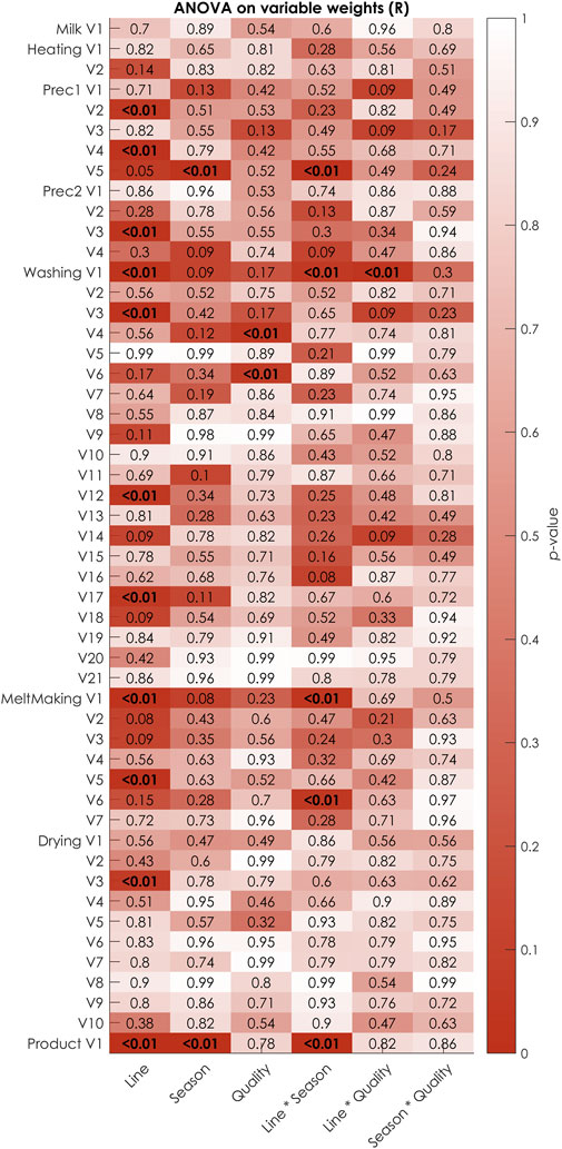
FIGURE 8. FDR-corrected$p$-values obtained by performing three-way ANOVA on the process variable weights (R) found with Process PLS according to the full factorial conditional path modelling approach. A low$p$-value signifies a low probability that the process variable weight is comparable under different (combinations of) production conditions.

For this demonstration, data was available for each combination of production conditions, but this may not be the necessarily hold for other production facilities. One parallel line may for instance never be used during winter, leading to a missing experiment in the design. In such cases, ANOVA may still be used to analyze the path modelling results, but Type I sums of squares should be used rather than Type III sums of squares. Alternatively, if including one operation condition causes too many missing experiments, it may be better to remove it altogether from the analysis. A parallel line that is only used during winter is for instance less insightful to include, and could be excluded from the analysis. Another solution could be to adapt the Process PLS model specification and include the operation condition as a process variable. It should furthermore be ensured that enough samples are present for each of the experiments to enable a reliable estimation of the process relationships with Process PLS for the corresponding combination of production conditions. A minimum of 30 samples is used for the demonstration given and is advisable, but the robustness of the fitted process relationships should in any case be assessed by analyzing the bootstrapping results as the minimum number of samples required will be process-specific.

Conclusion

This study presented a systematic approach for conditional path modelling of industrial production data using Process PLS, and demonstrated its value for a milk powder production facility. The approach consists of separating historical data based on one or more operation conditions, and modelling and comparing each of those datasets. This can be used to investigate how the statistical relationships between the production steps of a plant vary for, for instance, different production lines, seasons and quality ranges, and which of the measured process variables in those steps are most correlated to this behavior. An unprecedented high level of process expert knowledge on the structure and operation of the plant can thus be incorporated in the analysis of large historical datasets. Results for conditional modelling on a single production condition at a time and on all production conditions simultaneously were presented. The latter requires more data for stable modelling, was shown to be preferred as it allows for the quantification of interaction effects of the production conditions on the process relationships. Such interactions were present for the demonstrator process, and interpreting them gave a very detailed insight into the plant operation. These insights can both confirm and expand the current understanding of the process. This is of high value to process operators and engineers, who can use this improved understanding to pinpoint shortcomings in the current process monitoring and control strategy. Although only demonstrated on a continuous process in the current work, conditional path modelling may also be of great value for (batch-like) process with multiple production stages by considering those stages as a production condition. Ultimately, conditional path modelling can help in making production plants less prone to variations in external operating conditions, and in increasing product quality even for production plants that are already considered well-controlled.

Data Availability Statement

The raw data supporting the conclusion of this article will be made available by the authors, without undue reservation.

Author Contributions

TO: Conceptualization, Methodology, Software, Validation, Formal analysis, Investigation, Data curation, Writing—original draft, Writing—review and editing, Visualization; LH: Conceptualization, Methodology, Formal analysis, Investigation, Writing—review and editing; GK: Conceptualization, Methodology, Writing—review and editing, Supervision; ES: Conceptualization, Methodology, Resources, Writing—review and editing, Visualization, Supervision, Project administration; LB: Supervision, Project administration, Funding acquisition; JJ: Conceptualization, Methodology, Writing—review and editing, Visualization, Supervision, Project administration, Funding acquisition.

Funding

This project is co-funded by TKI-E and I with the supplementary grant ‘TKI- Toeslag’ for Topconsortia for Knowledge and Innovation (TKI’s) of the Ministry of Economic Affairs and Climate Policy. The authors thank all partners within the project ‘Integrating Sensor Based Process Monitoring and Advanced Process Control (INSPEC)’, managed by the Institute for Sustainable Process Technology (ISPT) in Amersfoort, Netherlands.

Conflict of Interest

ES was employed by FrieslandCampina.

The remaining authors declare that the research was conducted in the absence of any commercial or financial relationships that could be construed as a potential conflict of interest.

Publisher’s Note

All claims expressed in this article are solely those of the authors and do not necessarily represent those of their affiliated organizations, or those of the publisher, the editors and the reviewers. Any product that may be evaluated in this article, or claim that may be made by its manufacturer, is not guaranteed or endorsed by the publisher.

Supplementary Material

The Supplementary Material for this article can be found online at: https://www.frontiersin.org/articles/10.3389/frans.2021.721657/full#supplementary-material

References

Benjamini, Y., and Hochberg, Y. (1995). Controlling the False Discovery Rate: A Practical and Powerful Approach to Multiple Testing. J. R. Stat. Soc. Ser. B (Methodological) 57 (1), 289–300. doi:10.1111/j.2517-6161.1995.tb02031.x

CrossRef Full Text | Google Scholar

Bersimis, S., Psarakis, S., and Panaretos, J. (2007). Multivariate Statistical Process Control Charts: An Overview. Qual. Reliab. Engng. Int. 23 (5), 517–543. doi:10.1002/qre.829

CrossRef Full Text | Google Scholar

Bylund, G. (1995). “Dairy Processing Handbook,” in Tetra Pak Processing Systems, Vol. G3. Tetra Pak Processing Systems AB. Available at: http://www.ales2.ualberta.ca/afns/courses/nufs403/PDFs/chapter15.pdf.

Google Scholar

Codesido, S., Hanafi, M., Gagnebin, Y., González-Ruiz, V., Rudaz, S., and Boccard, J. (2020). Network Principal Component Analysis: a Versatile Tool for the Investigation of Multigroup and Multiblock Datasets. Bioinformatics 37, 1297–1303. doi:10.1093/bioinformatics/btaa954

CrossRef Full Text | Google Scholar

Cuentas, S., Peñabaena-Niebles, R., and Garcia, E. (2017). Support Vector Machine in Statistical Process Monitoring: a Methodological and Analytical Review. Int. J. Adv. Manuf Technol. 91 (1–4), 485–500. doi:10.1007/s00170-016-9693-y

CrossRef Full Text | Google Scholar

de Jong, S. (1993). SIMPLS: An Alternative Approach to Partial Least Squares Regression. Chemometrics Intell. Lab. Syst. 18 (3), 251–263. doi:10.1016/0169-7439(93)85002-X

CrossRef Full Text | Google Scholar

Gade, K., Geyik, S. C., Kenthapadi, K., Mithal, V., and Taly, A. (2019). “Explainable AI in Industry,” in Proceedings of the ACM SIGKDD International Conference on Knowledge Discovery and Data Mining, 3203–3204. doi:10.1145/3292500.3332281

CrossRef Full Text | Google Scholar

Guo, S., Pang, K., and Qin, S. (2019). Least Angle Regression and Partial Least Squares Regression on Process Data and High Collinearity. Foundations Process Analytics Machine Learn. 57, 201682944. https://api.semanticscholar.org/CorpusID:201682944.

Google Scholar

Hair, J. F., Ringle, C. M., and Sarstedt, M. (2011). PLS-SEM: Indeed a Silver Bullet. J. Marketing Theor. Pract. 19 (2), 139–152. doi:10.2753/MTP1069-6679190202

CrossRef Full Text | Google Scholar

Höskuldsson, A., Rodionova, O., and Pomerantsev, A. (2007). Path Modeling and Process Control. Chemometrics Intell. Lab. Syst. 88 (1), 84–99. doi:10.1016/j.chemolab.2006.09.010

CrossRef Full Text | Google Scholar

Huitson, A., Dunn, O. J., and Clark, V. A. (1976). Applied Statistics: Analysis of Variance and Regression. The Statistician 25 (Issue 3), 236. Wiley. doi:10.2307/2987845

CrossRef Full Text | Google Scholar

Johnson, R. W. (2001). An Introduction to the Bootstrap. Teach. Stat. 23 (Issue 2), 49–54. CRC press. doi:10.1111/1467-9639.00050

CrossRef Full Text | Google Scholar

Kadlec, P., Gabrys, B., and Strandt, S. (2009). Data-driven Soft Sensors in the Process Industry. Comput. Chem. Eng. 33 (4), 795–814. doi:10.1016/j.compchemeng.2008.12.012

CrossRef Full Text | Google Scholar

Kourti, T. (2005). Application of Latent Variable Methods to Process Control and Multivariate Statistical Process Control in Industry. Int. J. Adapt. Control. Signal. Process. 19 (4), 213–246. doi:10.1002/acs.859

CrossRef Full Text | Google Scholar

Lauzon-Gauthier, J., Manolescu, P., and Duchesne, C. (2018). The Sequential Multi-Block PLS Algorithm (SMB-PLS): Comparison of Performance and Interpretability. Chemometrics Intell. Lab. Syst. 180, 72–83. doi:10.1016/J.CHEMOLAB.2018.07.005

CrossRef Full Text | Google Scholar

MacGregor, J. F., and Kourti, T. (1995). Statistical Process Control of Multivariate Processes. Control. Eng. Pract. 3 (3), 403–414. doi:10.1016/0967-0661(95)00014-L

CrossRef Full Text | Google Scholar

MATLAB (2017). The Math Works (Natick, Massachusetts: Inc). R2017a ed.

Offermans, T., Szymańska, E., Buydens, L. M. C., and Jansen, J. J. (2020). Synchronizing Process Variables in Time for Industrial Process Monitoring and Control. Comput. Chem. Eng. 140, 106938. doi:10.1016/j.compchemeng.2020.106938

CrossRef Full Text | Google Scholar

Qin, S. J. (1997). “Neural Networks for Intelligent Sensors and Control - Practical Issues and Some Solutions,” in Neural Systems for Control. Editors O. Omidvar, and D. L. Elliott (Academic Press), 213–234. doi:10.1016/b978-012526430-3/50009-x

CrossRef Full Text | Google Scholar

Romano, R., Tomic, O., Liland, K. H., Smilde, A., and Næs, T. (2019). A Comparison of twoPLS‐based Approaches to Structural Equation Modeling. J. Chemometrics 33 (3), e3105. doi:10.1002/cem.3105

CrossRef Full Text | Google Scholar

Souza, F. A. A., Araújo, R., and Mendes, J. (2016). Review of Soft Sensor Methods for Regression Applications. Chemometrics Intell. Lab. Syst. 152, 69–79. doi:10.1016/j.chemolab.2015.12.011

CrossRef Full Text | Google Scholar

Team R Development Core (2018). “A Language and Environment for Statistical Computing,” in R Foundation for Statistical Computing, Vol. 2. 3.6.3. Available at: https://www.R-project.org..

Google Scholar

van Kollenburg, G., Bouman, R., Offermans, T., Gerretzen, J., Buydens, L., van Manen, H.-J., et al. (2021). Process PLS: Incorporating Substantive Knowledge into the Predictive Modelling of Multiblock, Multistep, Multidimensional and Multicollinear Process Data Manuscript Revision Printed in Blueblue. Comput. Chem. Eng. 154, 107466. doi:10.1016/J.COMPCHEMENG.2021.107466

CrossRef Full Text | Google Scholar

van Kollenburg, G. H., Bouman, R., Offermans, T., and Jansen, J. (2020b). Data, Software and Scripts Related to the Process PLS Methodology Manuscript. Mendeley Data. doi:10.17632/9x9h7fr4kn.1

CrossRef Full Text | Google Scholar

van Kollenburg, G. H., van Es, J., Gerretzen, J., Lanters, H., Bouman, R., Koelewijn, W., et al. (2020a). Understanding Chemical Production Processes by Using PLS Path Model Parameters as Soft Sensors. Comput. Chem. Eng. 139, 106841. doi:10.1016/j.compchemeng.2020.106841

CrossRef Full Text | Google Scholar

Varmuza, K., and Filzmoser, P. (2016). Introduction to Multivariate Statistical Analysis in Chemometrics. Taylor & Francis Group, LLC. doi:10.1201/9781420059496

CrossRef Full Text

Zhang, Y., Zhou, H., Qin, S. J., and Chai, T. (2010). Decentralized Fault Diagnosis of Large-Scale Processes Using Multiblock Kernel Partial Least Squares. IEEE Trans. Ind. Inf. 6 (1), 3–10. doi:10.1109/TII.2009.2033181

CrossRef Full Text | Google Scholar