A Combined Lidar-Polarimeter Inversion Approach for Aerosol Remote Sensing Over Ocean

Introduction

Aerosols are tiny particles suspended in the atmosphere. They stem from a variety of natural and anthropogenic sources and processes, and influence the distribution of radiation by either directly absorbing, scattering and emitting radiation or indirectly by providing cloud condensation nuclei. In addition, the concentration and speciation of aerosols in the boundary layer impact air quality and consequently public health. Characterization of spatial and temporal variations of a few key aerosol characteristics such as abundance, size, absorption, and composition is critical for quantifying their global and regional impact on climate and air quality. However, the short life cycle of aerosols and high-degree of variability in their composition and distribution has been a challenge for their accurate remote sensing. According to the most recent IPCC report (IPCC, 2013), aerosols remain the largest radiative forcing uncertainty.

To better anchor aerosol direct and indirect impacts on the Earth’s energy balance, the Global Climate Observing System (GCOS, 2011) sets out observational requirements for a few key aerosol characteristics such as aerosol optical depth (AOD, denoted by “τ”), single scattering albedo (SSA), extinction profiles and layer height. For example, the accuracy of AOD at 550 nm is required to be better than the max of (0.1τ, 0.03) at the horizontal resolution of 5–10 km and a temporal resolution of 4 h. The accuracy of SSA is required to be better than 0.03. Aerosol extinction profiles are required to be better than 10% at a horizontal resolution of 200–500 km, a vertical resolution <1 km near the tropopause and of ∼2 km in the middle stratosphere. The NASA Aerosol Clouds, and Convection and Precipitation (ACCP) mission that is currently undergoing formulation (https://vac.gsfc.nasa.gov/accp/home.htm) is also setting up criteria on a set of geophysical variables (documented as Milestone SATM, September 16, 2019). For example, the total and planetary boundary layer (PBL) effective total fine mode AODs are desired to be better than 0.05τ_total/fine + 0.02. In both column and PBL effective sense, the accuracy of SSA is desired to be better than 0.03; aerosol extinction-to-backscatter ratios are required to be better than 25%; the real part of aerosol refractive index is desired to be better than 0.025; and the nonspherical AOD fractions are desired to be better than 10%. Aerosol extinction profile is desired to be better than the max of (0.02 km⁻¹, 20%–40%) at the vertical resolution from 30 to 250 m, depending on specific mission objective.

Capitalizing on the rapid advancement of lidar and polarimetric remote sensing techniques and the relevant remote sensing theory over the last few decades, the combination of these two types of measurement is highly promising for meeting the requirements described above. As an active remote sensing technique, lidar sends out laser pulses into atmosphere and detects the backscattered radiation. Accounting for speed of light, the time delay in the received signals determines the distance from the backscatter location, and the range-resolved profiles of attenuated backscatter (e.g., CALIOP (Winker et al., 2007)) or backscatter, extinction and depolarization (e.g., the measurement by the High Spectral Resolution Lidar (HSRL, (Hair et al., 2001; Hair et al., 2008; Rogers et al., 2009) at single or multiple wavelengths resolves aerosol types and microphysical properties, and consequently vertically resolved radiative forcing. The determination of vertically resolved aerosol radiative forcing has direct implications for the thermodynamic structure of atmosphere and consequent effects on monsoonal circulations and the global hydrological cycle. Polarimeters, in contrast, use the Sun as the radiation source and measure radiometric and polarimetric signals of sunlight reflection from top-of-atmosphere (TOA) in multi-spectral/hyper-spectral and multi-angular dimensions. It enables a moderate-to-high horizontal resolution aerosol/cloud optical and microphysical products during daytime. The global coverage of aerosol products enables its wide applications such as aerosol-cloud interaction and air quality studies. Like a radiometer, a polarimeter can provide large swath aerosol/cloud context for TOA flux assessment. Both theoretical studies and real data analysis have proved polarimeter’s capability of constraining column effective aerosol abundance, absorption and microphysical properties together with surface reflection properties (see for example [Mishchenko et al., 2011; Hasekamp et al., 2011; Chowdhary et al., 2012; Knobelspiesse et al., 2012; Dubovik et al., 2019; Remer et al., 2019; among others]). Compared to lidar, however, polarimeter carries much less information about the vertical distributions of aerosols.

It is apparent that lidar and polarimeter have highly complementary strengths: while lidar resolves details of aerosol vertical profiles and types, polarimeter provides constraints on anchoring column-effective aerosol abundance, absorption and microphysical properties across a large swath. Consequently, a combination of these two types of measurements enhances the observational information about aerosol properties. Informing aerosol retrieval by these two types of measurements, we target a comprehensive determination of aerosol size, type, abundance and absorption as well as their vertical variations.

To fully utilize the information contained in lidar and polarimetric measurements, reliable forward and inversion models are prerequisite. Some earlier efforts have been made toward combining lidar and polarimetric/radiometric measurements to improve the retrieval of aerosol properties. For example, Knobelspiesse et al. (2011) investigated the Research Scanning Polarimeter (RSP, Cairns et al., 1999) and HSRL (Hair et al., 2008) data collected during the field campaign - Arctic Research of the Composition of the Troposphere from Aircraft and Satellites (ARCTAS). It is found that the combined use of the two types of measurement in retrieval reduces the likelihood of unsuccessful retrievals caused by significantly biased initial estimate of the aerosol number concentration in optimal estimate inversion approach. In the case of ground-based observations, the LIRiC and GARRLiC algorithms have been developed by Chaikovsky et al. (2016) and by Lopatin et al. (2013), respectively. The latter is currently a branch of the Generalized Retrieval of Aerosol and Surface Properties (GRASP) algorithm (Dubovik et al., 2011; Dubovik et al., 2014). These two algorithms use joint data from a multi-wavelength lidar and an AERONET radiometer and derive two vertical profiles of fine and coarse aerosol components as well as extra parameters on the column-integrated properties of aerosols. Particularly, LIRIC derives vertical profiles using the retrieval results from AERONET but not changing them. GARRLiC/GRASP, on the other hand, fits simultaneously lidar and photometer data and derives both enhanced vertical and columnar aerosol properties. As ongoing efforts, Liu et al., (2016) and Burton et al., (2019) have been developing an optical estimate approach to retrieve vertically resolved particle concentrations, effective radius, and absorption by using both RSP and HSRL observations acquired during DISCOVER-AQ, TCAP and ORACLES field missions. Espinosa et al., (2019) used the GRASP algorithm to simulate the retrieval of attenuated backscatter lidar measurements in 532 and 1,064 nm in combination with a radiometer or polarimeter with 10 angles spaced over ±57° with 6 wavelengths spanning 0.44–2.2 μm. Compared to stand alone polarimetric or radiometric retrieval, an enhanced accuracy in fine mode aerosol SSA was observed from the combined retrieval. In essence, the combined retrieval capitalizes on the benefit of backscatter observations that contain sensitivity to the profiling properties of aerosols and the benefits of polarimetric observations that contain information about aerosol loading and absorption.

In this paper, we describe a research algorithm that allows a combined use of lidar and polarimetric observations for retrieving vertical profiles of speciated aerosol abundance and aerosol intrinsic properties such as size distribution, refractive index, and spherical particle fraction. The algorithm builds upon our earlier work using only polarimetric observations to retrieve a column effective set of aerosol properties over ocean (Xu et al., 2016). The paper is organized as follows. Following an algorithm overview in General Structure of the Algorithm, we introduce our 1D RT model for polarized RT in a coupled atmosphere-ocean system in Aerosol Scattering and Ocean Surface Reflection. Forward Model for Light Propagation in a Coupled Atmosphere-Ocean System formulates the inversion and error estimate approach. In Coupled Retrieval of Aerosols and Ocean Properties, we test the inversion algorithm using 50 sets of coincident lidar and polarimetric observations made by the HSRL-2 and RSP instruments aboard the NASA ER-2 during the NASA’s ORACLES field campaign (Redemann et al., 2021). These observations cover a moderately high bio-mass burning and sea salt aerosol loading with column total AOD_532-nm between ∼0.2 and ∼0.3 and an altitude dependent SSA. Comparisons of the retrieved AOD, SSA, and aerosol size distribution are made to the reference data measured by 4-STAR and HiGEAR which are aboard the NASA P-3 aircraft. A summary is given in Retrieval Implementation and Validation.

General Structure of the Algorithm

The combined lidar and polarimetric retrieval of aerosol loading and properties consists of three major modules: 1) A static light scattering dataset for intrinsic aerosol properties including refractive index and multiple rectangular size bins. The dataset is pre-calculated and called during the inversion to provide on-the-fly single scattering properties for spherical and nonspherical particle properties. These properties include aerosol optical depth, phase matrix and SSA for radiative transfer modeling; and extinction, backscatter and depolarization to fit lidar measurement; 2) A hybrid radiative transfer model that combines the computational strengths of the Markov-chain and adding-doubling approaches in modeling polarized RT in vertically inhomogeneous and homogeneous media, respectively; and 3) Optimization model. The inversion is assisted by allowing an imposition of smoothness constraints on the vertical variations of speciated aerosol refractive index, size parameters and spherical particle fraction. Following retrieval success and the output of the optimized solution, ancillary aerosol quantities including AOD, SSA, particulate lidar ratio, particulate extinction and backscatter coefficients as well as particulate depolarization are derived. Error estimate is provided for all retrieval outcome.

With these algorithm modules, we outlined in Figure 1 the algorithm flow of combined lidar-polarimeter inversion. Input into the retrieval consists of 1) lidar signals including extinction, backscatter, and/or depolarization or a subset of them; and 2) polarimetric signals including multi-angle and multi-spectral measurements of radiance and polarimetric components. As retrieval parameters, the state vector contains the column volume concentrations of multiple aerosol species and vertical profiles of 1) speciated aerosol refractive index with its spectral dependence constrained by a linear model in logarithmic space; 2) speciated log-normal volume weighted size distribution constrained by median size parameter and standard deviation; 3) species dependent spherical particle volume fraction; and 4) species column concentrations in vertical layers. Also included in the retrieval state vector are chlorophyll-a (Chl-a) concentration, an empirical spectral term that adjusts the water-leaving radiances to mitigate bio-optical modeling error, and the wind speed.

FIGURE 1

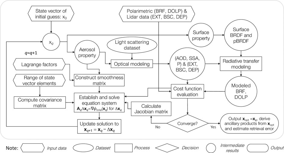
FIGURE 1. Algorithm flowcharts for retrieving aerosol and surface properties from a combined use of lidar and polarimer.

Our retrieval starts with an initialized state vector x₀. Speciated aerosol abundance, optical properties and microphysical properties are used to calculate vertically resolved aerosol single scattering quantities including 1) AOD, SSA and phase matrix for radiative transfer modeling and fit polarimetric measurement of radiance and degree of linear polarizartion (DOLP); and 2) aerosol extinction coefficient, scattering coefficient and depolarization ratio for fitting relevant lidar measurements. To guide the direction of search of solution through iterations, we run the forward model multiple times to calculate the Jacobian matrix that contains the derivatives of radiative and lidar quantities with respect to the aerosol and ocean surface properties. Moreover, a smoothness matrix is constructed to improve monotonic convergence of iteration toward the vicinity of globally optimized solution. A linear system is then established that includes the difference between model and observation, the Jacobian matrix, the smoothness matrix and the a priori. By solving the linear system, a stepwise increment of solution is determined to adjust the solution. In an iterative way, retrieval converges to a final solution.

Aerosol Scattering and Ocean Surface Reflection

Dependent on the information content offered by specific combinations of lidar and polarimeter, our algorithm is designed to be flexible in the aspect of allowing multiple aerosol species to be retrieved. In this section we will introduce the calculation of aerosol single scattering quantities as well as ocean surface reflection.

Adopting a log-normal volumetric size distribution $\left[d{v}_l^{\left(s\right)}\left(r\right)/d\ln r\right]$ for all (N_s) aerosol species, we have the subcolumn volumetric concentrations in lth layer,

$\frac{d{V}_l\left(r\right)}{d\ln r}={\displaystyle \sum _{s=1}^{N_s}{C}_{v,l}^{\left(s\right)}\frac{d{v}_l^{\left(s\right)}\left(r\right)}{d\ln r}},(1)$

where the size distribution of the sth species $d{v}_l^{\left(s\right)}\left(r\right)/d\ln r$ is parameterized by a geometric volume mean radius $r_m^{\left(s\right)}$ and a logarithmic standard deviation ${\sigma }_{m,l}^{\left(s\right)}$:

$\frac{d{v}_l^{\left(s\right)}\left(r\right)}{d\ln r}=\frac{1}{\sqrt{2\pi }{\sigma }_{m,l}^{\left(s\right)}}\exp \left[-\frac{{\left(\ln r-\ln r_{m,l}^{\left(s\right)}\right)}^2}{2{\left({\sigma }_{m,l}^{\left(s\right)}\right)}^2}\right].(2)$

In Eq. 1, $C_{v,l}^{\left(s\right)}$ is the subcolumn volume concentration of the sth aerosol species in the lth layer and is related to its volume fraction $\left(f_{v,l}^{\left(s\right)}\right)$ and the total column concentration $\left(C_v^{\mathrm{tot},\left(s\right)}\right)$ by $C_{v,l}^{\left(s\right)}=C_v^{\mathrm{tot},\left(s\right)}{f}_{v,l}^{\left(s\right)}$.

If we discretize the speciated aerosol size distribution in the lth layer into N_bin size bins, the volumetric fraction of the ith bin is equal to $f_{i,l}^{\left(s\right)}d\ln r_i$ (1 ≤ i ≤ N_bin), where $f_{i,l}^{\left(s\right)}$ is calculated by

$f_{i,l}^{\left(s\right)}=\frac{d{v}_l^{\left(s\right)}\left(r_i\right)}{d\ln r_i},(3)$

where r_i stands for the central radius of ith size bin and $d{v}_l^{\left(s\right)}\left(r_i\right)/d\ln r_i$ can be evaluated from Eq. 2.

Aerosol Single Scattering Properties for Radiative Transfer Calculation

In this section, we are going to introduce the calculation of aerosol single scattering properties including AOD, SSA and phase matrix elements for radiative transfer modeling.

Accounting for the contribution by both spherical and spheroid-based nonspherical particles, the volumetric extinction coefficient $K_{\mathrm{e}\mathrm{x}\mathrm{t},a,l}^{\left(s\right)}$ and scattering coefficient $K_{\mathrm{s}\mathrm{c}\mathrm{a},a,l}^{\left(s\right)}$ (in the unit of m⁻¹) are calculated by

$K_{\mathrm{e}\mathrm{x}\mathrm{t},a,l}^{\left(s\right)}=K_{\mathrm{e}\mathrm{x}\mathrm{t},a,l}^{\left(s\right),\mathrm{sphere}}+K_{\mathrm{e}\mathrm{x}\mathrm{t},a,l}^{\left(s\right),\mathrm{spheroid}}(4)$

for sth aerosol species. In the above equation, the volumetric extinction component of spherical particles is evaluated by

$\begin{array}{l}{K}_{\mathrm{e}\mathrm{x}\mathrm{t},a,l}^{\left(s\right),\mathrm{sphere}}=C_{n_0,a,l}^{\left(s\right),\mathrm{sphere}}{\displaystyle {\int }_{r_{\min }}^{r_{\max }}\frac{d{n}_l^{\left(s\right)}\left(r\right)}{d\ln r}{c}_{\mathrm{e}\mathrm{x}\mathrm{t},a,l}^{\left(s\right),\mathrm{sphere}}\left(m_{a,l}^{\left(s\right)},r\right)d\ln r}\\ =C_{v_0,a,l}^{\left(s\right)}{f}_{v,l}^{\left(s\right),\mathrm{sphere}}{\displaystyle {\int }_{r_{\min }}^{r_{\max }}\frac{d{v}_l^{\left(s\right)}\left(r\right)}{d\ln r}\frac{1}{v\left(r\right)}{c}_{\mathrm{ext},a,l}^{\left(s\right),\mathrm{sphere}}\left(m_{a,l}^{\left(s\right)},r\right)d\ln r,}\end{array}(5)$

where $C_{n_0,a,l}^{\left(s\right),\mathrm{sphere}}$ is the aerosol number concentration (m⁻³), $d{n}_l^{\left(s\right)}\left(r\right)/d\ln r$ is the number weighted aerosol size distribution in association with $d{v}_l^{\left(s\right)}\left(r\right)/d\ln r$, r_min and r_max are the lower and upper bounds of the size distribution respectively, $c_{\mathrm{e}\mathrm{x}\mathrm{t},a,l}^{\left(s\right),\mathrm{sphere}}$ is extinction cross section as a function of particle refractive index $m_{a,l}^{\left(s\right)}$ and radius r, $f_{v,l}^{\left(s\right),\mathrm{sphere}}$ is the volume fraction of spherical particles, v(r) is the volume of a spherical particle of radius r, and $C_{v_0,a,l}^{\left(s\right)}$ is the aerosol volumetric concentration (in the unit of m³/m³). It is related to the subcolumn aerosol concentration ($C_{v,a,l}^{\left(s\right)}$ in the unit of m³/m²) in lth layer by

$C_{v,a,l}^{\left(s\right)}=C_{v_0,a,l}^{\left(s\right)}\Delta H_l=C_v^{\mathrm{tot},\left(s\right)}{f}_{v,l}^{\left(s\right)},(6)$

where

$f_{v,l}^{\left(s\right)}=\frac{C_{v,l}^{\left(s\right)}\Delta H_l}{C_v^{\mathrm{tot},\left(s\right)}}=\frac{C_{v,l}^{\left(s\right)}\Delta H_l}{{\displaystyle \sum _{l=1}^{N_{Layer}}{C}_{v,l}^{\left(s\right)}\Delta H_l}}.(7)$

Calculation of volumetric extinction coefficient of spheroidal particles in Eq. 4 should account for both size and aspect ratio distributions of spheroids (Dubovik et al., 2011). Therefore,

$\begin{array}{l}{K}_{\mathrm{ext},a,l}^{\left(s\right),\mathrm{spheroid}}=C_{n_0,a,l}^{\left(s\right),\mathrm{spheroid}}{\displaystyle {\int }_{r_{\min }}^{r_{\max }}\frac{d{n}_l^{\left(s\right)}\left(r\right)}{d\ln r}{c}_{\mathrm{ext},a,l}^{\left(s\right),\mathrm{spheroid}}(m_{a,l}^{\left(s\right)},r)d\ln r}\\ =C_{v_0,a,l}^{\left(s\right)}(1-f_{v,l}^{\left(s\right),\mathrm{sphere}}){\displaystyle {\int }_{{\eta }_{\min }}^{{\eta }_{\max }}{\displaystyle {\int }_{r_{\min }}^{r_{\max }}\frac{d{n}_l^{\left(s\right)}\left(\eta \right)}{d\ln \eta }\frac{d{v}_l^{\left(s\right)}\left(r\right)}{d\ln r}\frac{1}{v\left(r\right)}{c}_{\mathrm{ext},a,l}^{\left(s\right),\mathrm{spheroid}}(m_{a,l}^{\left(s\right)},r,\eta )d\ln \eta d\ln r}}\end{array}(8)$

where r becomes the volume equivalent spherical particle radius, the aspect ratio η < 1 for oblate spheroids and η > 1 for prolate spheroids, and η_min and η_max are the lower and upper bounds of the aspect ratio distribution respectively. Note that we assume spheroids to have fixed aspect ratio distribution (Legrand et al., 2014) and $d{n}_l^{\left(s\right)}\left(\eta \right)/d\ln \eta$ is independent of aerosol size. Both $d{n}_l^{\left(s\right)}\left(\eta \right)/d\ln \eta$ and $d{v}_l^{\left(s\right)}\left(r\right)/d\ln r$ are normalized to unity in the presence of non-zero lower bound or non-infinity upper bound in their integral over r and η, respectively.

For numerical calculation, the aerosol size distribution is descritized into N_bin rectangular bins so that for spherical particles

$K_{\mathrm{ext},a,l}^{\left(s\right),\mathrm{shere}}=C_{v_0,a,l}^{\left(s\right)}{f}_{v,l}^{\left(s\right),\mathrm{sphere}}{\displaystyle \sum _{i=1}^{N_{\mathrm{b}\mathrm{i}\mathrm{n}}}\frac{d{v}_l^{\left(s\right)}\left(r_i\right)}{d\ln r}{K}_{\mathrm{ext},a,l,i}^{\left(s\right),\mathrm{sphere}}(m_{a,l}^{\left(s\right)},r_i)},(9)$

where the component of sth aerosol species in its ith size bin is

$K_{\mathrm{ext},a,l,i}^{\left(s\right),\mathrm{sphere}}(m_{a,l}^{\left(s\right)},r_i)={\int }_{\ln r_i-\Delta \ln r_i/2}^{\ln r_i+\Delta \ln r_i/2}\frac{c_{\mathrm{ext},a,l}^{\left(s\right),\mathrm{sphere}}(m_{a,l}^{\left(s\right)},r)}{v\left(r\right)}\mathrm{d}\ln r.(10)$

For spheroids, we further need to break the integral of volumetric extinction into N_AR bins of aspect ratio so that:

$K_{\mathrm{ext},a,l}^{\left(s\right),\mathrm{spheroid}}=C_{v_0,a,l}^{\left(s\right)}(1-f_{v,l}^{\left(s\right),\mathrm{shere}}){\displaystyle \sum _{i=1}^{N_{\mathrm{b}\mathrm{i}\mathrm{n}}}{K}_{\mathrm{ext},a,l,i}^{\left(s\right),\mathrm{spheroid}}(m_{a,l}^{\left(s\right)},r_i)\frac{d{v}_l^{\left(s\right)}\left(r_i\right)}{d\ln r}},(11)$

where

$K_{\mathrm{ext},a,l,i}^{\left(s\right),\mathrm{spheroid}}(m_{a,l}^{\left(s\right)},r_i)={\displaystyle \sum _{q=1}^{N_{\mathrm{A}\mathrm{R}}}\frac{d{n}_l^{\left(s\right)}\left({\eta }_q\right)}{d\ln \eta }{\int }_{\ln {\eta }_q-\Delta \ln \eta q/2}^{\ln {\eta }_q+\Delta \ln \eta q/2}{\int }_{\ln r_i-\Delta \ln ri/2}^{\ln r_i+\Delta \ln ri/2}\frac{c_{\mathrm{ext},a,l}^{\left(s\right),\mathrm{spheroid}}(m_{a,l}^{\left(s\right)},r,\eta )}{v\left(r\right)}}\mathrm{d}\ln r\mathrm{d}\ln \eta .(12)$

For simplicity, the layer resolved volumetric extinction coefficient can be rewritten in the following form,

$K_{\mathrm{ext},a,l}^{\left(s\right)}={\displaystyle \sum _{i=1}^{N_{\mathrm{b}\mathrm{i}\mathrm{n}}}{f}_{i,l}^{\left(s\right)}\left[f_{v,l}^{\left(s\right),\mathrm{sphere}}{K}_{\mathrm{ext},a,l,i}^{\left(s\right),\mathrm{sphere}}+(1-f_{v,l}^{\left(s\right),\mathrm{sphere}})K_{\mathrm{ext},a,l,i}^{\left(s\right),\mathrm{spheroid}}\right]},(13)$

where $K_{\mathrm{ext},a,l,i}^{\left(s\right),\mathrm{sphere}}$ and $K_{\mathrm{ext},a,l,i}^{\left(s\right),\mathrm{spheroid}}$ are given in Eqs 10 and 12, respectively.

Replacing the subscript “ext” by “sca” in above derivations (Eqs. 4–13) gives relevant equations for the volumetric scattering coefficient:

$K_{\mathrm{sca},a,l}^{\left(s\right)}={\displaystyle \sum _{i=1}^{N_{\mathrm{b}\mathrm{i}\mathrm{n}}}{f}_{i,l}^{\left(s\right)}\left[f_{v,l}^{\left(s\right),\mathrm{sphere}}{K}_{\mathrm{sca},a,l,i}^{\left(s\right),\mathrm{sphere}}+(1-f_{v,l}^{\left(s\right),\mathrm{sphere}})K_{\mathrm{sca},a,l,i}^{\left(s\right),\mathrm{spheroid}}\right]}.(14)$

In a similar way, the phase matrix element P_a,j,k,l of sth aerosol species in the lth layer is calculated from

$P_{a,j,k,l}^{\left(s\right)}=\frac{{\displaystyle \sum _{i=1}^{N_{bin}}{f}_{i,l}^{\left(s\right)}\left[f_{v,l}^{\left(s\right),\mathrm{sphere}}{K}_{a,\mathrm{sca},l,i}^{\left(s\right),\mathrm{sphere}}{P}_{a,j,k,l,i}^{\left(s\right),\mathrm{sphere}}+\left(1-f_{v,l}^{\left(s\right),\mathrm{sphere}}\right)K_{a,\mathrm{sca},l,i}^{\left(s\right),\mathrm{spheroid}}{P}_{a,j,k,l,i}^{\left(s\right),\mathrm{spheroid}}\right]}}{{\displaystyle \sum _{i=1}^{N_{bin}}{f}_{i,l}^{\left(s\right)}\left[f_{v,l}^{\left(s\right),\mathrm{sphere}}{K}_{a,\mathrm{sca},l,i}^{\left(s\right),\mathrm{sphere}}+\left(1-f_{v,l}^{\left(s\right),\mathrm{sphere}}\right)K_{a,\mathrm{sca},l,i}^{\left(s\right),\mathrm{spheroid}}\right]}}.(15)$

In the numerator of the above equation, we have

$K_{\mathrm{sca},a,l,i}^{\left(s\right),\mathrm{sphere}}{P}_{a,j,k,l,i}^{\left(s\right),\mathrm{sphere}}={\int }_{\ln r_i-\Delta \ln r_i/2}^{\ln r_i+\Delta \ln r_i/2}\frac{c_{\mathrm{sca},a,l}^{\left(s\right),\mathrm{sphere}}(m_{a,l}^{\left(s\right)},r)}{v\left(r\right)}{P}_{a,j,k,l}^{\left(s\right),\mathrm{sphere}}(m_{a,l}^{\left(s\right)},r)\mathrm{d}\ln r,(16)$

$K_{\mathrm{sca},a,l,i}^{\left(s\right),\mathrm{spheroid}}{P}_{a,j,k,l,i}^{\left(s\right),\mathrm{spheroid}}={\displaystyle \sum _{q=1}^{N_{AR}}\frac{d{n}_l^{\left(s\right)}\left({\eta }_q\right)}{d\ln \eta }{\int }_{\ln {\eta }_q-\Delta \ln \eta q/2}^{\ln {\eta }_q+\Delta \ln \eta q/2}{\int }_{\ln r_i-\Delta \ln r_i/2}^{\ln r_i+\Delta \ln r_i/2}\frac{c_{\mathrm{sca},a,l}^{\left(s\right),\mathrm{spheroid}}(m_{a,l}^{\left(s\right)},r,\eta )}{v\left(r\right)}{P}_{a,j,k,l,q}^{\left(s\right),\mathrm{spheroid}}(m_{a,l}^{\left(s\right)},r,\eta )}\mathrm{d}\ln r\mathrm{d}\ln \eta .(17)$

Summing over the contributions from all aerosol species gives the total volumetric extinction and scattering coefficients in lth layer,

$K_{\mathrm{ext}\left[\mathrm{sca}\right],a,l}={\displaystyle \sum _{s=1}^{N_s}{K}_{\mathrm{ext}\left[\mathrm{sca}\right],a,l}^{\left(s\right)}},(18)$

where $K_{\mathrm{ext},a,l}^{\left(s\right)}$ and $K_{\mathrm{sca},a,l}^{\left(s\right)}$ are given by Eqs 13 and 14 respectively.

The speciated aerosol SSA in lth layer is calculated as the ratio of speciated scattering and extinction coefficients by,

${\omega }_{0,a,l}^{\left(s\right)}=\frac{K_{\mathrm{sca},a,l}^{\left(s\right)}}{K_{\mathrm{ext},a,l}^{\left(s\right)}}.(19)$

Contributed by all aerosol species, the overall SSA contributed by all aerosol species in lth layer is

${\omega }_{0,a,l}=\frac{{\displaystyle \sum _{s=1}^{N_s}{f}_{v,l}^{\left(s\right)}{K}_{\mathrm{sca},a,l}^{\left(s\right)}}}{{\displaystyle \sum _{s=1}^{N_s}{f}_{v,l}^{\left(s\right)}{K}_{\mathrm{ext},a,l}^{\left(s\right)}}},(20)$

where $f_{v,l}^{\left(s\right)}$ stands for the volume fraction of sth aerosol species in lth layer, as given by Eq. 7.

The overall aerosol phase matrix elements are evaluated by,

$P_{a,j,k,l}=\frac{{\displaystyle \sum _{s=1}^{N_s}{f}_{v,l}^{\left(s\right)}{K}_{\mathrm{sca},a,l}^{\left(s\right)}}{P}_{a,j,k,l}^{\left(s\right)}}{{\displaystyle \sum _{s=1}^{N_s}{f}_{v,l}^{\left(s\right)}{K}_{\mathrm{sca},a,l}^{\left(s\right)}}},(21)$

where $P_{a,j,k,l}^{\left(s\right)}$ is given by Eq. 15. The layer aerosol optical depth (AOD, $\Delta {\tau }_{a,l}$) is contributed by all aerosol species. Therefore, we have

$\Delta {\tau }_{a,l}={\displaystyle \sum _{s=1}^{N_s}\Delta {\tau }_{a,l}^{\left(s\right)}}.(22)$

In the above equation, the AOD for sth aerosol species is

$\Delta {\tau }_{a,l}^{\left(s\right)}=C_{v,a,l}^{\left(s\right)}{K}_{\mathrm{ext},a,l}^{\left(s\right)},(23)$

where $C_{v,a,l}^{\left(s\right)}$ is the subcolumn volumetric concentration of sth aerosol species, evaluated by Eq. 6, and $K_{\mathrm{ext},a,l}^{\left(s\right)}$ is column effective extinction coefficient (in the unit of m⁻¹) of sth aerosol species in the lth layer, evaluated by Eq. 13.

Aerosol Single Scattering Properties for Lidar Equation Use

In this section, we are going to introduce the calculation of aerosol single scattering properties including extinction, backscatter and depolarization for use in the lidar equation.

The total extinction coefficient for lth layer (${\alpha }_{a,l}$, in the unit of m⁻¹) is calculated by summing over the contribution from all aerosol species, namely

${\alpha }_{a,l}={\displaystyle \sum _{s=1}^{N_s}{\alpha }_{a,l}^{\left(s\right)}},(24)$

where the speciated aerosol extinction ${\alpha }_{\text{a,}l}^{\left(s\right)}$ in a layer of geometric thickness ΔH_l is related to layer resolved aerosol optical depth by

${\alpha }_{a,l}^{\left(s\right)}=\frac{\Delta {\tau }_{a,l}^{\left(s\right)}}{\Delta H_l}=\frac{C_{v,a,l}^{\left(s\right)}{K}_{\mathrm{ext},a,l}^{\left(s\right)}}{\Delta H_l},(25)$

where $C_{v,a,l}^{\left(s\right)}$ and $K_{\mathrm{ext},a,l}^{\left(s\right)}$ are given by Eqs 6 and 7 respectively.

Calculation of the total backscatter ${\beta }_{a,l}$ (in the unit of m⁻¹Sr⁻¹) also needs to account for the contributions of all aerosol species as well, namely

${\beta }_{a,l}={\displaystyle \sum _{s=1}^{N_s}{\beta }_{a,l}^{\left(s\right)}},(26)$

where the speciated aerosol backscatter is evaluated by

${\beta }_{a,l}^{\left(s\right)}={\beta }_{\mathrm{sca},a,l}^{\left(s\right)}\frac{P_{a,\mathrm{1,1},l}^{\left(s\right)}\left({180}^{\circ }\right)}{4\pi },(27)$

where $P_{a,\mathrm{1,1},l}^{\left(s\right)}\left({180}^{\circ }\right)$ is given by Eq. 15 and the aerosol scattering coefficient (${\beta }_{\mathrm{sca},a,l}^{\left(s\right)}$, in the unit of m⁻¹) in lth layer is evaluated by,

${\beta }_{\mathrm{sca},a,l}^{\left(s\right)}=\frac{C_{v,a,l}^{\left(s\right)}{K}_{\mathrm{sca},a,l}^{\left(s\right)}}{\Delta H_l},(28)$

where $K_{\mathrm{sca},a,l}^{\left(s\right)}$ is given by Eq. 16.

Assuming random orientation of nonspherical particles, the aerosol linear depolarization ratio of lth layer is calculated as

${\delta }_{a,l}\left({180}^{\circ }\right)=\frac{1-P_{a,\mathrm{2,2},l}\left({180}^{\circ }\right)/P_{a,\mathrm{1,1},l}\left({180}^{\circ }\right)}{1+P_{a,\mathrm{2,2},l}\left({180}^{\circ }\right)/P_{a,\mathrm{1,1},l}\left({180}^{\circ }\right)},(29)$

where the layer resolved phase matrix elements P_a,i,j,l are evaluated via Eq. 21.

Development of a Lookup Table for Aerosol Single Scattering Properties

Calculation of aerosol single scattering properties (AOD, SSA, p) for RT modeling and (α_a, β_a, δ_a) for fitting lidar measurements needs to use the aerosol refractive index as the input. We adopt the following two parameter constrained model for refractive index as a function of wavelength (Dubovik and King, 2000),

$m_{r,l}\left(\lambda \right)=m_{r0,l}{(\lambda /{\lambda }_0)}^{-{\kappa }_{r0,l}}{m}_{i,l}\left(\lambda \right)=m_{i0,l}{(\lambda /{\lambda }_0)}^{-{\kappa }_{i0,l}}(30)$

where m_r0 and m_i0 are the real and imaginary parts of the refractive index at the reference wavelength λ₀, and κ_r0 and κ_i0 are used to characterize their spectral dependence.

During the optimization process, the spectrally dependent refractive index and size distribution of aerosols and the spherical particle fraction of aerosols are updated dynamically. To avoid inefficient on-the-fly light scattering computations of aerosol extinction [scattering] coefficients $K_{\mathrm{ext}\left[\mathrm{sca}\right],a,i}^{\mathrm{sphere}\left[\mathrm{spheroid}\right]}$, and aerosol phase matrix $P_{\text{a},j,k\text{,}i}^{\text{sphere}\left[\text{spheroid}\right]}$ are precalculated for a set of size bins and refractive indices and saved in a lookup table. The table is then linearly interpolated to determine the scattering properties associated with dynamically updated refractive index during the retrieval. The bin resolved properties are weighted by size distribution parameters to determine $K_{\mathrm{ext}\left[\mathrm{sca}\right],a,i}^{\text{sphere}\left[\text{spheroid}\right]}$, $P_{\text{a},j,k\text{,}i}^{\text{sphere}\left[\text{spheroid}\right]}$ and then (α_a, β_a, δ_a) for the whole size distribution (see Aerosol Single Scattering Properties for Radiative Transfer Calculation and Aerosol Single Scattering Properties for Lidar Equation Use).

In the generation of the lookup table, the real part of refractive index is uniformly distributed in linear space from 1.3 to 1.7 with 22 grids. The imaginary part of refractive index is uniformly distributed in logarithmic space from 1 × 10⁻⁸ to 3 × 10⁻⁴ with five grids and from 5 × 10⁻⁴ to 0.5 with 15 grids. The lower and upper bounds for aerosol size are set as r_min = 5 nm and r_max = 50 μm, respectively. A total of 50 size bins are equally spaced in logarithmic space to calculate aerosol light scattering properties. Mie theory is used to calculate spherical particle scattering (van de Hulst, 1981). For spheroids, the lower and upper bounds for aerosol axis ratio to be 0.33 and 3.0 respectively and a total of 25 bins are set for precalculating spheroidal scattering properties by use of T-matrix method in combination with geometric optics (Dubovik et al., 2006).

Surface Reflection

The use of bio-optical model to simulate ocean water-leaving radiance effectively reduces the parameter space and provides extra constraints in the retrieval of ocean bulk properties. It has been more and more adopted over the last decade and justified by many research groups (see for example [Chowdhary et al., 2012; Xu et al., 2016; Gao et al., 2018; Stamnes et al., 2018; among others]). Our ocean surface reflection model incorporates a polarized specular reflection term, a Lambertian term for depolarizing ocean foam reflection and an empirical Lambertian correction term “Δa” to account for the errors of the single-parameter based bio-optical model (i.e., departures from the predetermined functional relationships to Chl-a). The overall bidirectional ocean surface reflection matrix R_surf is described by (Xu et al., 2016),

$\text{π}{\mathbf{R}}_{\text{Surf,}\lambda }=f_{\text{Foam}}{a}_{\text{Foam,}\lambda }{\mathbf{D}}_{\text{0}}+(1-f_{\text{Foam}}){\mathbf{R}}_{\text{W,}\lambda }+(1-f_{\text{Foam}}){\mathbf{R}}_{\text{WL,}\lambda }^{\text{Bio}}+(1-f_{\text{Foam}})\Delta a_{\text{WL,}\lambda }{\mathbf{D}}_{\text{0}},(31)$

where D₀ is a zero matrix except D_0,11 = 1; a_Foam is foam albedo; f_Foam is foam coverage fraction related to wind speed V_wind by f_Foam = 2.95 × 10⁻⁶×V_wind^3.52 (Koepke, 1984); R_W,λ is the polarized specular reflection from water surface (Cox and Munk, 1954a; Cox and Munk, 1954b), and ${\mathbf{R}}_{\text{WL},\lambda }^{\text{Bio}}$ is the reflection matrix of the ocean-interface system with a correction of Raman scattering (Lee et al., 2013; Xu et al., 2016), and “Δa_WL,λ” is the Lambertian correction term. Note that ${\mathbf{R}}_{\text{WL,}\lambda }^{\text{Bio}}$ is a physically based term depending on the Chl-a concentration [Chl_a]. The last two terms of Eq. 31 constitute our water-leaving radiance model. With and without assuming Δa_WL to be 0 the simplified and the empirically adjusted bio-optical models are formulated, respectively. By setting the Sun at zenith and viewing angle to be nadir, we can evaluate the normalized water-leaving radiance from ${\mathbf{R}}_{\text{WL}}^{\text{Bio}}$ and Δa_WL,

$\mathrm{n}\mathrm{L}{\mathrm{w}}_{\lambda }=\frac{F_{0,\lambda }}{\pi }{\left(\frac{d_0}{d}\right)}^2\left[R_{\mathrm{WL},\lambda ,11}^{\mathrm{Bio}}({\theta }_v=0^{\circ };{\theta }_0=0^{\circ };[\mathrm{C}\mathrm{h}\mathrm{l}\_\mathrm{a}])+\Delta a_{\mathrm{WL},\lambda }\right],(32)$

where d₀ is the Earth-Sun distance at which F₀ is reported, and d is the Earth-Sun distance at the time of measurement. Note that nLw, ${\mathbf{R}}_{\mathbf{W}}$, R_surf, ${\mathbf{R}}_{\text{WL}}^{\text{Bio}}$, a_Foam, Δa_WL, and F₀ in Eqs 31 and 32 are all spectrally dependent.

Forward Model for Light Propagation in a Coupled Atmosphere-ocean System

Polarized Radiative Transfer

As illustrated in Figure 2, a coupled atmosphere-surface model is established for 1D RT modeling, which consists of an aerosol/air-molecule atmospheric layer and ocean water at the bottom of the atmosphere. The whole atmosphere is subdivided into N_Layer layers, each bounded by the altitudes h_l and h_l+1 (h_l < h_l+1) and N_Layer depends on the vertical resolution of lidar measurement or the desired resolution for retrieval products.

FIGURE 2

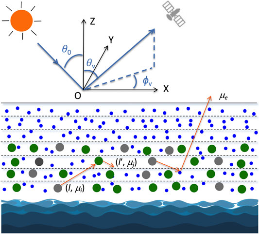
FIGURE 2. The coupled atmosphere-ocean system for RT modeling. The Sun illuminates the top of atmosphere with zenith angle θ₀ and azimuthal angle ϕ₀ (ϕ₀ is assumed to be zero here). The sensor views the atmosphere at viewing angle θ_v and azimuthal angle ϕ_v. The Markov chain model is used for computing polarized RT in the atmosphere. The ocean is assumed optically homogeneous so that the doubling method can be applied to achieve modeling efficiency. Coupling of local radiative fields from ocean and atmospheric layer is completed by using an “adding” strategy.

As the input to radiative transfer modeling, vertically resolved AOD, SSA, and phase matrices of aerosols in all layers are calculated from speciated aerosol refractive index, size distributions and spherical particle fraction. They are mixed with molecule scattering to get bulk scattering properties in all layers. Consequently, the optical thickness (Δτ_l), SSA (ω_0,l) and phase matrix (P_l) of lth layer contributed by both aerosols and Rayleigh-scattering molecules are evaluated by

$\Delta {\tau }_1=\Delta {\tau }_{a,1}+\Delta {\tau }_{R,1},(33)$

${\omega }_{0,l}=\frac{\Delta {\tau }_{R,l}+{\omega }_{0,a,l}\Delta {\tau }_{a,l}}{\Delta {\tau }_{R,l}+\Delta {\tau }_{a,l}},(34)$

${\mathbf{P}}_l\left(\Theta \right)=\frac{\Delta {\tau }_{\text{R,}l}{\mathbf{P}}_{\text{R}}\left(\Theta \right)+{\omega }_{0,\text{a,}l}\Delta {\tau }_{\text{a,}l}{\mathbf{P}}_{\text{a,}l}\left(\Theta \right)}{\Delta {\tau }_{\text{R,}l}+{\omega }_{0,\text{a,}l}\Delta {\tau }_{\text{a,}l}},(35)$

where as a function of scattering angle Θ, P_R and P_a,l are the Rayleigh and aerosol phase matrices, respectively, the aerosol SSA of lth layer (ω_0,a,l) is given by Eq. 20 and the AOD of lth layer (Δτ_a,l) is given by Eq. 22.

Knowing the layer optical depth, SSA and phase matrices for all atmospheric layers, an efficient calculation of reflection and transmission matrices of the vertically inhomogeneous atmosphere is implemented by use of the Markov chain method (Esposito and House, 1978; Esposito 1979; Xu et al., 2010; Xu et al., 2011; Xu et al., 2012). As an approximation, the ocean water constituents are assumed to be homogeneously mixed. Then the doubling method (see for example [Stokes, 1862; van de Hulst, 1963; Hansen, 1971; de Haan et al., 1987; Evans and Stephens, 1991; among others]) is applied for a fast calculation of the reflection matrices of the ocean bulk. Finally, the interaction between atmosphere and ocean through multiple reflection and transmission are coupled via an “adding” approach (Xu et al., 2016). The output of atmosphere and ocean reflection is the reflection matrix for the coupled atmosphere-ocean system, from which the radiance and polarimetric components are derived to compare to observations. The incorporation of Markov chain model and doubling methods into a hybrid RT modeling scheme capitalizes on the strength of these two methods in modeling RT in vertically inhomogeneous and homogeneous media, respectively. Moreover, it provides an efficient Jacobian calculation and an optimization-based retrieval by saving the local RT fields (reflection and transmission matrices) for each layer from forward modeling, which are then reused for subsequent Jacobian evaluations as long as the aerosol or ocean parameters remain unperturbed. In other words, only the RT in the layer with perturbed parameters requires recalculation.

Lidar Equation

The propagation of a light pulse from a single-channel lidar in the atmosphere is governed by lidar equation (e.g., (Winker et al., 1996; Vaughan, 2004; Weitkamp, 2005; Burton et al., 2018]):

$\frac{P_p\left(z\right)}{g_p}=\frac{1}{z^2}\left[{\beta }_{\mathrm{m}}\left(z\right)+{\beta }_{\mathrm{a}}\left(z\right)\right]\exp \left\{-2{\displaystyle {\int }_0^z\left[{\alpha }_{\mathrm{m}}\left(z^{\prime }\right)+{\alpha }_{\mathrm{a}}\left(z^{\prime }\right)\right]d{z}^{\prime }}\right\},(36)$

where $P_p\left(z\right)$ is the calibrated signal at the detector as a function of the range (distance, z) between the lidar and the target atmospheric volume, g_p is a gain factor which takes into account detector and receiver optical efficiencies, β_a(z) and β_m(z) are backscatter coefficients of aerosols and air molecules at range z, and ${\alpha }_{\text{a}}$ and ${\alpha }_{\text{m}}$ are the aerosol and molecular extinction coefficients respectively. The exponential term on the right-hand side of the above equation represents two-way attenuation of the lidar signal between the detector and the atmospheric volume.

The multiplication of the exponential term on the right hand side of Eq. 36 and the term “[β_a(z) + β_m(z)]” gives attenuated backscatter. The molecular scattering and extinction coefficients β_m(r) and α_m(r) can be accurately determined from measured atmospheric density or from climatology. What remain to be resolved are the aerosol extinction and backscatter coefficients. However, with these two unknowns coupled in the attenuated backscatter lidar system via Eq. 36, they cannot be separated from one measured variable on the left-hand-side of the equation. By adopting the HSRL measurement technique, however, the received backscatter is split into two channels, one with a very narrow bandwidth optical absorption filter in the molecular channel to suppress the aerosol backscatter, whereas another is a combined channel that detects the intensity contributed by both aerosol and molecules. In this case, the lidar equation for the combined signal remains the same as the above equation while for the molecular channel with narrow bandwidth optical absorption filter the lidar equation becomes [e.g., Burton et al., 2015],

$\frac{P_p\left(z\right)}{g_p}=\frac{1}{z^2}{\beta }_m\left(z\right)\exp \left\{-2{\displaystyle {\int }_0^z\left[{\alpha }_m\left(z^{\prime }\right)+{\alpha }_a\left(z^{\prime }\right)\right]d{z}^{\prime }}\right\}.(37)$

High-spectral-resolution lidars such as NASA Langley’s HSRL-1 and HSRL-2 send a linearly polarized beam into an atmosphere. The returned lidar signals are measured with linear polarization analyzers oriented both parallel (||) and perpendicular (⊥) to the emitted beam. By taking the ratio of light intensities of these two components, the depolarization ratio of the returned transmitted signal is derived as:

$\delta =\frac{I_{\perp }}{I_{\parallel }}.(38)$

Due to the anisotropy of the air molecules, the depolarization ratio of the pure molecular atmosphere is nonzero but can be pre-calculated from climatology. Moreover, the backscatter of a linearly polarized laser beam from spherical particles is totally linearly polarized so that (δ = 0). However, the presence of nonspherical aerosols causes the measured depolarization ratio to deviate from zero which provides extra constraints on retrieving non-sphericity of aerosols.

The lidar equation Eq. 37 is single scattering based. It can break into a discretized form, namely multiplication of local backscatter at range z with the sum of the contributions of extinction in all layers above z. The calculation of aerosol component of layer effective extinction (α_a), backscatter (β_a) and depolarization (δ_a) have been specified in Aerosol Single Scattering Properties for Lidar Equation Use. In addition, to combine lidar observations with polarimetric measurements: one can structure the retrieval to fit either direct lidar measurements such as total extinction, backscatter and depolarization, or its aerosol products such as particulate extinction, backscatter and depolarization ratio. The latter is adopted in the current retrieval demonstration in Retrieval Implementation and Validation.

Coupled Retrieval of Aerosols and Ocean Properties

State Vector

Our algorithm is developed to be flexible and allow for multiple (N_s) aerosol species to be retrieved from a combined use of lidar and polarimetric measurements depending on the information content of 1) the specific configuration of lidar measurement capabilities in terms of providing the whole set or a subset of extinction, backscatter/attenuated backscatter, and depolarization ratio measurements, their vertical resolutions and number of wavelengths; and 2) the number of radiometric and polarimetric view angles and spectral channels provided by a polarimeter. The state vector x that includes retrieval parameters for N_s aerosol species can be expressed as,

$\mathbf{x= }{\left[{\mathbf{x}}^{\left(1\right)};{\mathbf{x}}^{\left(2\right)};\cdots ;{\mathbf{x}}^{\left(N_s\right)};{\mathbf{x}}^{(\text{ocean})}\right]}_{N\times 1},(39)$

where N is the total number of aerosol and ocean properties to be retrieved, the subvector x^(s) contains aerosol properties for sth aerosol species. For a total of N_aer = 8 aerosol parameters per species, we have,

${\mathbf{x}}^{\left(s\right)}\mathbf{= }{\left[{\mathit{C}}_{\text{v}}^{\left(s\right)};{\mathit{m}}_{r_0}^{\left(s\right)};{\mathit{\kappa }}_{r_0}^{\left(s\right)};{\mathit{m}}_{i_0}^{\left(s\right)};{\mathit{\kappa }}_{i_0}^{\left(s\right)};{\mathit{r}}_{\text{m}}^{\left(s\right)};{\mathit{\sigma }}_{\text{m}}^{\left(s\right)};{\mathit{f}}_{\text{v}}^{\left(s\right)\text{,sphere}}\right]}_{N_{\text{aer}}\times 1},(40)$

where for sth aerosol species C_v contains layer specific column aerosol concentration (m³/m²), (m_r0, κ_r0) and (m_i0, κ_i0) are layer resolved model parameters that constrain spectrally dependent real and imaginary parts of aerosol refractive index, respectively (via Eq. 30); r_m and σ_m contain layer resolved geometric volume median radius and standard deviation of volumetric log-normal distribution; f_v^sphere contain the layer resolved volume fraction of spherical aerosols. As the last component of the state vector in Eq. 39, x^(ocean) contains parameters that contribute to ocean surface reflection. These parameters include a simplified bio-optical model parameter chlorophyll-a concentration, wind speed and the empirical terms (Lambertian) that mitigate the bio-optical modeling errors by adjusting the spectral water-leaving radiance (see Development of a Lookup Table for Aerosol Single Scattering Properties). Retrieval starts with an initial estimate of these parameters, as specified in Table 1.

TABLE 1

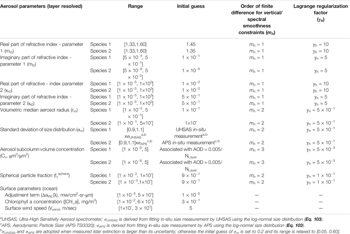
TABLE 1. Parameters in coupled aerosol and surface property retrieval, their initial estimates, and order of difference and Lagrange multipliers for imposing smoothness constraints.

Constraints

Imposition of various types of constraints is important for stabilizing the retrievals and improving accuracy. The combined lidar-polarimeter inversion approach described here uses three types of constraints: 1) direct observation signals provided by lidar and polarimetric remote sensing measurements (see formulation in Observational Constraints (i = 1)); 2) a priori constraint for the retrieval parameters (see formulation in A Priori Constraints (i = 2)); and 3) smoothness constraint over the variations of certain aerosol properties along altitude (see formulation in Smoothness Constraints (i = 3)). Incorporation of all these three types of constraints into our combined inversion approach is described in Construction of Overall Equation System.

Imposition of the above three types of constraints (M = 3) can be formulated in the framework of statistical inversion of multi-source constraints. Our objective is to solve the following system of equations (Dubovik, 2004):

${\mathbf{f}}_i^{\ast }={\mathbf{f}}_i\left(\mathbf{x}\right)+\Delta {\mathbf{f}}_i^{\ast },1\le i\le M(41)$

where ${\mathbf{f}}_i^{\ast }$ denotes the $i^{\text{th}}$ type of constraint, $\Delta {\mathbf{f}}_i^{\ast }$ is the error with this type of constraint, and x = x_state as defined in Eq. 39. Formally, the statistical independence of different sources of constraints means that the covariance matrix of joint constraint $\mathbf{f}\ast =[{\mathbf{f}}_1^{\ast };{\mathbf{f}}_2^{\ast };\cdots ;{\mathbf{f}}_M^{\ast }]$ has the following structure

${\mathbf{C}}_{f^{\ast }}=\left[\begin{array}{cccc}{\mathbf{C}}_1& \mathbf{0}& \mathbf{0}& \mathbf{0}\\ \mathbf{0}& {\mathbf{C}}_2& \mathbf{0}& \mathbf{0}\\ \cdots & \cdots & \ddots & \cdots \\ \mathbf{0}& \mathbf{0}& & {\mathbf{C}}_M\end{array}\right],(42)$

where C_i indicates the covariance matrix of the ith constraint (${\mathbf{f}}_i^{\ast }$). Following the expressions of ${\mathbf{f}}_i^{\ast }$ and ${\mathbf{C}}_{{\mathbf{f}}_i^{\ast }}$, the probability distribution function (PDF) of joint data (1 ≤ i ≤ M) can be derived by multiplying PDFs of data from all M sources of constraints, namely,

$\text{P}\left(\mathbf{f}\left(\mathbf{x}\right)\right|{\mathbf{f}}^{\ast })={\displaystyle \prod _{i=1}^M\text{P}\left({\mathbf{f}}_i\left(\mathbf{x}\right)\right|{\mathbf{f}}_i^{\ast })}\sim \exp \left\{-\frac{1}{2}{\displaystyle \sum _{i=1}^M{\left[{\mathbf{f}}_i\left(\mathbf{x}\right)-{\mathbf{f}}_i^{\ast }\right]}^{\text{T}}{\left({\mathbf{C}}_i\right)}^{-1}\left[{\mathbf{f}}_i\left(\mathbf{x}\right)-{\mathbf{f}}_i^{\ast }\right]}\right\}.(43)$

Further introducing the weight matrix (W), the objective cost function to be minimized has a quadratic form, namely,

${\Psi }_{\text{total}}\left(\mathbf{x}\right)={\displaystyle \sum _{i=1}^M{\gamma }_i{\Psi }_i\left(\mathbf{x}\right)},(44)$

where

${\Psi }_i\left(\mathbf{x}\right)=\frac{1}{2}{\left[{\mathbf{f}}_i\left(\mathbf{x}\right)-{\mathbf{f}}_i^{\ast }\right]}^{\text{T}}{\mathbf{W}}_i^{-1}\left[{\mathbf{f}}_i\left(\mathbf{x}\right)-{\mathbf{f}}_i^{\ast }\right],(45)$

with

${\mathbf{W}}_i=\frac{1}{{\epsilon }_i^2}{\mathbf{C}}_i,(46)$

${\gamma }_i=\frac{{\epsilon }_1^2}{{\epsilon }_i^2},(47)$

In the above equations, ${\epsilon }_i^2$ is the first diagonal element of C_i (i.e., ${\epsilon }_i^2={\left\{C_i\right\}}_{11}$) and the Lagrange factor ${\gamma }_i$ weights the contribution of each type of constraint with respective to the first one (${\gamma }_1=1$).

Minimization of ${\Psi }_{\text{total}}\left(\mathbf{x}\right)$ in Eq. 44 means its gradient with respect to the solution x approaches zero, such that

$\nabla {\Psi }_{\text{total}}\left(\mathbf{x}\right)={\displaystyle \sum _{i=1}^M{\gamma }_i\nabla {\Psi }_i\left(\mathbf{x}\right)}=0,(48)$

which can be ensured by enforcing the gradient of all components approach zero, namely

$\nabla {\Psi }_i\left(\mathbf{x}\right)={\mathbf{K}}_i^{\text{T}}{\mathbf{W}}_i^{-1}({\mathbf{f}}_i\left(\mathbf{x}\right)-{\mathbf{f}}_i^{\ast })=0,(49)$

where ${\mathbf{K}}_i$ is the Jacobian matrix containing the derivatives of the ith type of constraint with respect to the retrieval parameters. To approach the solution iteratively, we replace x by x − Δx in Eq. 49 and substitute

${\mathbf{f}}_i(\mathbf{x}-\Delta \mathbf{x})={\mathbf{f}}_i\left(\mathbf{x}\right)-{\mathbf{K}}_i\Delta \mathbf{x},(50)$

into it. This results in

$\nabla {\Psi }_i(\mathbf{x}-\Delta \mathbf{x})={\mathbf{K}}_i^{\text{T}}{\mathbf{W}}_i^{-1}({\mathbf{f}}_i\left(\mathbf{x}\right)-{\mathbf{K}}_i\Delta \mathbf{x}-{\mathbf{f}}_i^{\ast })=0,(51)$

or equivalently,

$({\mathbf{K}}_i^{\text{T}}{\mathbf{W}}_i^{-1}{\mathbf{K}}_i\mathbf{)}\Delta \mathbf{x}={\mathbf{K}}_i^{\text{T}}{\mathbf{W}}_i^{-1}({\mathbf{f}}_i\left(\mathbf{x}\right)-{\mathbf{f}}_i^{\ast })=\nabla {\Psi }_i\left(\mathbf{x}\right).(52)$

The Jacobian matrix ${\mathbf{K}}_i$ in Eqs 49–52 consists of the derivative of the mth observational or a priori data with respect to the nth unknown,

$K_{i,(m,n)}=\frac{\partial f_{i,m}}{\partial x_n}.(53)$

More explicit evaluation of ${\mathbf{f}}_i\left(\mathbf{x}\right)$, ${\mathbf{f}}_i^{\ast }$ and K and W matrices for all types of constraints is discussed in the following subsections.

Observational Constraints (i = 1)

Without the loss of generality, we assume a polarimeter measures multi-angular radiance (L) across multiple spectral channels. Neglecting the contribution from circular polarization, the polarimetric components Q/L and U/L can be combined into DOLP via DOLP = (Q² + U²)^1/2/L. Lidar observations include extinction (α), backscatter or attenuated backscatter (β) and depolarization ratio (δ). Arranging all types of observations into a single column vector we have

${\mathbf{f}}_{i=1}^{\ast }\left(\mathbf{x}\right)=\left({\mathbf{f}}_{1,L}^{\ast };{\mathbf{f}}_{1,\text{DOLP}}^{\ast };{\mathbf{f}}_{1,\alpha }^{\ast };{\mathbf{f}}_{1,\beta }^{\ast };{\mathbf{f}}_{1,\delta }^{\ast }\right)=[y_1;y_2;\cdots ;y_{N_{\text{f}}}],(54)$

where the total number of signals N_f = N_L + N_DOLP + N_α + N_β + N_δ, where N_x is the number of “x” type of signals.

The aerosol and ocean properties in the state vector are adjusted so that the model prediction of these types of signals ${\mathbf{f}}_1\left(\mathbf{x}\right)=[{\mathbf{f}}_{1\text{, L}};{\mathbf{f}}_{1\text{, DOLP}};{\mathbf{f}}_{1,\alpha };{\mathbf{f}}_{1,\beta };{\mathbf{f}}_{1,\delta }]$ fit the observational constraints ${\mathbf{f}}_1^{\ast }\left(\mathbf{x}\right)$. The calculation of ${\mathbf{f}}_1\left(\mathbf{x}\right)$ is introduced in Forward Model for Light Propagation in a Coupled Atmosphere-Ocean System. The Jacobian matrix K₁ consists of first order partial derivatives with respect to all elements in the state vector x, namely,

${\mathbf{K}}_1={\left[\begin{array}{ccccc}{\mathbf{K}}_{\text{L}}& {\mathbf{K}}_{\text{DOLP}}& {\mathbf{K}}_{\alpha }& {\mathbf{K}}_{\beta }& {\mathbf{K}}_{\delta }\end{array}\right]}^{\text{T}},(55)$

where K_L, K_DOLP, K_α, K_β, and K_δ are the Jacobian matrices containing derivatives of L, DOLP, α, β and δ with respect to aerosol parameters x_j (1 ≤ j ≤ N), respectively. Accounting for all N parameters in the state vector (see Eq. 39), K_L can be expanded into the following matrix form:

${\mathbf{K}}_{\text{L}}=\left[\begin{array}{cccc}\frac{\partial L_1}{\partial x_1}& \frac{\partial L_1}{\partial x_2}& \cdots & \frac{\partial L_1}{\partial x_N}\\ \frac{\partial L_2}{\partial x_1}& \frac{\partial L_2}{\partial x_2}& \cdots & \frac{\partial L_2}{\partial x_N}\\ \cdots & \cdots & \ddots & \cdots \\ \frac{\partial L_{N_L}}{\partial x_1}& \frac{\partial L_{N_L}}{\partial x_2}& \cdots & \frac{\partial L_{N_L}}{\partial x_N}\end{array}\right],(56)$

where N_L depends on the number of views angles (N_view) and the number of channels (N_{λ, L}) of a polarimeter. Assuming the same number of view angles for all spectral bands, then we have N_L = N_λ,L × N_view. Replacing “L” in the above equation by DOLP gives the Jacobian matrix K_DOLP and in this case the total number of DOLP signals depends on the number of polarimetric bands (N_λ,DOLP) so that N_DOLP = N_λ,DOLP × N_view. Calculation of the derivatives in Eq. 56 can proceed numerically by use of finite difference method, or analytically (and more efficiently) if the RT model is linearized.

The Jacobian matrix for extinction coefficient equals to

${\mathbf{K}}_{\alpha }=\left[\begin{array}{ccccc}{\mathbf{K}}_{\alpha ,l=1}& \mathbf{0}& \cdots & \mathbf{0}& \mathbf{0}\\ \mathbf{0}& {\mathbf{K}}_{\alpha ,l=2}& \cdots & \mathbf{0}& \mathbf{0}\\ ⋮& ⋮& \ddots & ⋮& ⋮\\ \mathbf{0}& \mathbf{0}& \cdots & {\mathbf{K}}_{\alpha ,l=N_{\text{Layer}}}& \mathbf{0}\\ \mathbf{0}& \mathbf{0}& \cdots & \mathbf{0}& {\mathbf{0}}_{\text{Ocean}}\end{array}\right],(57)$

where N_Layer is the number of layers in which lidar signals are resolved. Assuming extinction α is provided at M_α wavelengths, the layer resolved Jacobian matrix (${\mathbf{K}}_{\alpha ,l}$) for extinction coefficient equals to,

${\mathbf{K}}_{\alpha ,l}=\left[\begin{array}{cccc}\frac{\partial {\alpha }_l\left({\lambda }_1\right)}{\partial x_{l,1}}& \frac{\partial {\alpha }_l\left({\lambda }_1\right)}{\partial x_{l,2}}& \cdots & \frac{\partial {\alpha }_l\left({\lambda }_1\right)}{\partial x_{l,N}}\\ \frac{\partial {\alpha }_l\left({\lambda }_2\right)}{\partial x_{l,1}}& \frac{\partial {\alpha }_l\left({\lambda }_2\right)}{\partial x_{l,2}}& \cdots & \frac{\partial {\alpha }_l\left({\lambda }_2\right)}{\partial x_{l,N}}\\ \cdots & \cdots & \ddots & \cdots \\ \frac{\partial {\alpha }_l\left({\lambda }_{M_{\alpha }}\right)}{\partial x_{l,1}}& \frac{\partial {\alpha }_l\left({\lambda }_{M_{\alpha }}\right)}{\partial x_{l,2}}& \cdots & \frac{\partial {\alpha }_l\left({\lambda }_{M_{\alpha }}\right)}{\partial x_{l,N}}\end{array}\right],(58)$

The Jacobian matrix for backscatter coefficient and attenuated backscatter coefficients is evaluated by,

${\mathbf{K}}_{\beta }=\left[\begin{array}{cccc}{\mathbf{K}}_{\beta ,l=1}& \mathbf{0}& \cdots & \mathbf{0}\\ \mathbf{0}& {\mathbf{K}}_{\beta ,l=2}& \cdots & \mathbf{0}\\ \cdots & \cdots & \ddots & \cdots \\ \mathbf{0}& \mathbf{0}& \cdots & {\mathbf{K}}_{\beta ,l=N_{\text{Layer}}}\end{array}\right],(59)$

and

${\mathbf{K}}_{\beta }=\left[\begin{array}{cccc}{\mathbf{K}}_{\beta ,l=1}& \mathbf{0}& \cdots & \mathbf{0}\\ {\mathbf{K}}_{\beta ,l=1}& {\mathbf{K}}_{\beta ,l=2}& \cdots & \mathbf{0}\\ \cdots & \cdots & \ddots & \cdots \\ {\mathbf{K}}_{\beta ,l=1}& {\mathbf{K}}_{\beta ,l=2}& \cdots & {\mathbf{K}}_{\beta ,l=N_{\text{Layer}}}\end{array}\right],(60)$

respectively. Assuming β is provided at M_β wavelengths, the layer resolved Jacobian matrix for backscatter coefficient (${\mathbf{K}}_{\beta ,l}$) can be expanded into the following specific form,

${\mathbf{K}}_{\beta ,l}=\left[\begin{array}{cccc}\frac{\partial {\beta }_l\left({\lambda }_1\right)}{\partial x_{l,1}}& \frac{\partial {\beta }_l\left({\lambda }_1\right)}{\partial x_{l,2}}& \cdots & \frac{\partial {\beta }_l\left({\lambda }_1\right)}{\partial x_{l,N}}\\ \frac{\partial {\beta }_l\left({\lambda }_2\right)}{\partial x_{l,1}}& \frac{\partial {\beta }_l\left({\lambda }_2\right)}{\partial x_{l,2}}& \cdots & \frac{\partial {\beta }_l\left({\lambda }_2\right)}{\partial x_{l,N}}\\ \cdots & \cdots & \ddots & \cdots \\ \frac{\partial {\beta }_l\left({\lambda }_{M_{\beta }}\right)}{\partial x_{l,1}}& \frac{\partial {\beta }_l\left({\lambda }_{M_{\beta }}\right)}{\partial x_{l,2}}& \cdots & \frac{\partial {\beta }_l\left({\lambda }_{M_{\beta }}\right)}{\partial x_{l,N}}\end{array}\right],(61)$

where β = β_l,a if we use the derived product of particulate backscatter for the lth layer from lidar measurement, and β = β_l,att if we used direct measured attenuated backscatter signals, where β_l,att is the product of the backscatter (contributed by both molecules and aerosols) and the two-way transmission of the atmospheric volume between the lidar and the backscatter volume in question (see Eq. 36).

The Jacobian matrix for depolarization ratio (δ) equals to

${\mathbf{K}}_{\delta }=\left[\begin{array}{cccc}{\mathbf{K}}_{\delta ,l=1}& \mathbf{0}& \cdots & \mathbf{0}\\ \mathbf{0}& {\mathbf{K}}_{\delta ,l=2}& \cdots & \mathbf{0}\\ \cdots & \cdots & \ddots & \cdots \\ \mathbf{0}& \mathbf{0}& \cdots & {\mathbf{K}}_{\delta ,l=N_{\text{Layer}}}\end{array}\right].(62)$

Assuming extinction δ is provided at M_δ wavelengths, the layer resolved Jacobian matrix for depolarization ratio (${\mathbf{K}}_{\delta ,l}$) equals to

${\mathbf{K}}_{\delta ,l}=\left[\begin{array}{cccc}\frac{\partial {\delta }_l\left({\lambda }_1\right)}{\partial x_{l,1}}& \frac{\partial {\delta }_l\left({\lambda }_1\right)}{\partial x_{l,2}}& \cdots & \frac{\partial {\delta }_l\left({\lambda }_1\right)}{\partial x_{l,N}}\\ \frac{\partial {\delta }_l\left({\lambda }_2\right)}{\partial x_{l,1}}& \frac{\partial {\delta }_l\left({\lambda }_2\right)}{\partial x_{l,2}}& \cdots & \frac{\partial {\delta }_l\left({\lambda }_2\right)}{\partial x_{l,N}}\\ \cdots & \cdots & \ddots & \cdots \\ \frac{\partial {\delta }_l\left({\lambda }_{M_{\delta }}\right)}{\partial x_{l,1}}& \frac{\partial {\delta }_l\left({\lambda }_{M_{\delta }}\right)}{\partial x_{l,2}}& \cdots & \frac{\partial {\delta }_l\left({\lambda }_{M_{\delta }}\right)}{\partial x_{l,N}}\end{array}\right].(63)$

where δ_l is contributed by both molecules and aerosols in lth layer and is equal to particulate depolarization ratio (δ = δ_l,a) if the derived aerosol depolarization ratio is used directly.

The overall covariance matrix incorporates the submatrices from all types of signals, namely,

${\mathbf{W}}_1=\left[\begin{array}{ccccc}{\mathbf{W}}_{\text{L}}& \mathbf{0}& \mathbf{0}& \mathbf{0}& \mathbf{0}\\ \mathbf{0}& {\mathbf{W}}_{\text{DOLP}}& \mathbf{0}& \mathbf{0}& \mathbf{0}\\ \mathbf{0}& \mathbf{0}& {\mathbf{W}}_{\alpha }& \mathbf{0}& \mathbf{0}\\ \mathbf{0}& \mathbf{0}& \mathbf{0}& {\mathbf{W}}_{\beta }& \mathbf{0}\\ \mathbf{0}& \mathbf{0}& \mathbf{0}& \mathbf{0}& {\mathbf{W}}_{\delta }\end{array}\right],(64)$

If absolute measurement uncertainty is used and correlation among signals are neglected, then W_x is a diagonal matrix. Taking jth signal (x_j) with relative uncertainty σ_j as an example, we have W_{x, jj} = ${\sigma }_j^2$. If relative uncertainty (ε_j) is used, then we have W_{x, jj} = ${\epsilon }_j^2{x}_j^2$. Under certain circumstances signals may differ in magnitude. To balance their contributions to the cost function which reflects the quality of fitting, observations are often transferred to logarithmic space for fitting. In this case, we have W_{x, jj} = ${\epsilon }_j^2$.

A Priori Constraints (i = 2)

Starting from Eq. 41, the a priori constraint can be explicitly expressed as (Dubovik, 2004),

${\mathbf{f}}_{i=2}^{\ast }={\mathbf{x}}^{apriori}=\mathbf{x}+\Delta {\mathbf{x}}^{apriori}.(65)$

Moreover, ${\mathbf{K}}_{i=2}$ = I (identity matrix) and ${\mathbf{W}}_{i=2}=\left(1/{\epsilon }_{a_{11}^{\ast }}^2\right){\mathbf{C}}_{a\ast }$ in Eqs 49–52. In explicit form, ${\mathbf{W}}_{i=2}$ is constructed from estimated range of each parameter relative to the first one (Dubovik and King, 2000),

${\mathbf{W}}_{i=2}={\mathbf{W}}_a=\left[\begin{array}{cccc}1& 0& \cdots & 0\\ 0& \frac{{(x_{2,\max }-x_{2,\min })}^2}{{(x_{1,\max }-x_{1,\min })}^2}& \cdots & 0\\ \cdots & \cdots & \ddots & \cdots \\ 0& 0& \cdots & \frac{{(x_{N,\max }-x_{N,\min })}^2}{{(x_{1,\max }-x_{1,\min })}^2}\end{array}\right].(66)$

where [x_i,min, x_i,max] are the lower and upper bounds of ith retrieval parameters, respectively. For retrieving combined RSP and HSRL-2 observations, their estimates are specified in Table 1.

Smoothness Constraints (i = 3)

The third type of constraint reflects the smooth variation of a certain type of parameter as a function of altitude. we have

${\mathbf{f}}_3^{\ast }={\mathbf{0}}^{\ast }={\mathbf{S}}_{i=3,m}\mathbf{x }+{\Delta }_g^{\ast },(67)$

where S_i=3,m is the differentiation matrix of mth order for third type of constraint and the delta term ${\Delta }_g^{\ast }$ accounts for the uncertainties associated with the assumption of smooth variation of an aerosol parameter to the mth order. The error of such an assumption is accounted via the cost function component given in Eq. 75 later.

When a retrieval parameter varies smoothly as a function of some variable (e.g., altitude) z, it is assumed to be locally approximated by a smooth function g(z), such as a constant, a line, a parabola, etc. With a polynomial form, the mth derivative approaches zero (Dubovik et al., 2011), such that,

$\{S_{i,m}\left(z\right)z=\frac{{\text{d}}^{m}g\left(z\right)}{\text{d}{z}^m}=0\Rightarrow \{\begin{array}{l}{g}_{m\mathrm{=1}}\left(z\right)=\text{const}\\ g_{m\mathrm{=2}}\left(z\right)=Az+B\\ g_{m\mathrm{=3}}\left(z\right)=A{z}^2+Bz+C\end{array}.(68)$

For a discretized grid of the variable z, the explicit form of S_i,mz, is,

$S_{i,m}\left(z_j\right)z_j=\{\begin{array}{l}\frac{\text{d}g}{\text{d}z}\approx \frac{{\Delta }^{1}g}{{\Delta }_1\left(z\right)}=\frac{g\left(z_{j+1}\right)-g\left(z_j\right)}{{\Delta }_1\left(z_j\right)},\text{ for }m=1\\ \frac{{\text{d}}^{m}g}{\text{d}{z}^m}\approx \frac{{\Delta }^{m}g}{{\Delta }_m\left(z\right)}=\frac{{\Delta }^{m-1}g\left(z_{j+1}\right)/{\Delta }_{m-1}\left(z_{j+1}\right)-{\Delta }^{m-1}g\left(z_j\right)/{\Delta }_{m-1}\left(z_j\right)}{[{\Delta }_{m-1}\left(z_j\right)+{\Delta }_{m-1}\left(z_{j+1}\right)]/2},\text{ for }m\ge 2\end{array}.(69)$

Taking the orders of difference m = 1 and 2 as examples, we have

$\{\begin{array}{l}{\Delta }_{m=1}\left(z_j\right)=z_{j+1}-z_j\\ {\Delta }_{m=2}\left(z_j\right)=[{\Delta }_1\left(z_j\right)+{\Delta }_1\left(z_{j+1}\right)]/2\end{array}.(70)$

Application of the above equation to L discretized grids r_j (namely, 1 ≤ j ≤ L) leads to

${\mathbf{f}}_i\left(\mathbf{x}\right)={\mathbf{S}}_{i,m}\mathbf{x},(71)$

so that by invoking Eq. 53,

${\mathbf{K}}_i={\mathbf{S}}_{i,m},(72)$

where the matrix S_i,m is evaluated by,

${\mathbf{S}}_{i,m=1}=\left[\begin{array}{ccccc}\frac{1}{{\Delta }_1\left(1\right)}& -\frac{1}{{\Delta }_1\left(1\right)}& 0& \cdots & 0\\ 0& \frac{1}{{\Delta }_1\left(2\right)}& -\frac{1}{{\Delta }_1\left(2\right)}& \cdots & 0\\ 0& 0& \cdots & \ddots & 0\\ 0& 0& \cdots & \frac{1}{{\Delta }_1(L-1)}& -\frac{1}{{\Delta }_1(L-1)}\end{array}\right],(73)$

and

$\mathbf{S}i,m=2=\left[\begin{array}{ccccccc}\frac{2}{{\Delta }_1\left(1\right)[{\Delta }_1\left(1\right)+{\Delta }_1\left(2\right)]}& \frac{-2}{{\Delta }_1\left(1\right){\Delta }_1\left(2\right)}& \frac{2}{{\Delta }_1\left(2\right)[{\Delta }_1\left(1\right)+{\Delta }_1\left(2\right)]}& 0& 0& \cdots & 0\\ 0& \frac{2}{{\Delta }_1\left(2\right)[{\Delta }_1\left(2\right)+{\Delta }_1\left(3\right)]}& \frac{-2}{{\Delta }_1\left(2\right){\Delta }_1\left(3\right)}& \frac{2}{{\Delta }_1\left(3\right)[{\Delta }_1\left(2\right)+{\Delta }_1\left(3\right)]}& \cdots & 0\\ \cdots & \cdots & \cdots & \cdots & \cdots & \ddots & \cdots \\ 0& 0& \cdots & \frac{2}{{\Delta }_1(L-1)[{\Delta }_1(L-1)+{\Delta }_1\left(L\right)]}& \frac{-2}{{\Delta }_1(L-1){\Delta }_1\left(L\right)}& \cdots & \frac{2}{{\Delta }_1\left(L\right)[{\Delta }_1(L-1)+{\Delta }_1\left(L\right)]}\end{array}\right](74)$

The same principle applied to higher orders of difference (m > 2) ensures a smooth curve with $d^{m}g\left(z\right)/d{z}^m=0$. Substitution of Eqs 71 and 72 and ${\mathbf{f}}_i^{\ast }=\mathbf{0}\ast$ into Eq. 45 gives,

${\Psi }_i\left(\mathbf{x}\right)=\frac{1}{2}{\mathbf{x}}^{\text{T}}{\mathbf{S}}_{i,m}^{\text{T}}{\mathbf{W}}_{i,m}^{-1}{\mathbf{S}}_{i,m}\mathbf{x},(75)$

where the weighting matrix W has the following diagonal terms,

${\left\{{\mathbf{W}}_{i,m}\right\}}_{jj}=\frac{1}{{\Delta }_m\left(z_j\right)},(76)$

and ${\Delta }_m\left(z_j\right)$ is specified in Eq. 70 for m = 1 and 2, and can be generalized to an arbitrary higher order.

Substitution of Eqs 71 and 72 and ${\mathbf{f}}_i^{\ast }={\mathbf{0}}^{\ast }$ into Eq. 52 gives

$({\mathbf{S}}_{i,m}^{\text{T}}{\mathbf{W}}_{i,m}^{-1}{\mathbf{S}}_{i,m}\mathbf{)}\Delta \mathbf{x}={\mathbf{S}}_{i,m}^{\text{T}}{\mathbf{W}}_{i.m}^{-1}\left({\mathbf{S}}_{i,m}\mathbf{x}\right).(77)$

Further defining

${\mathbf{\Omega }}_i={\mathbf{S}}_{i,m}^{\text{T}}{\mathbf{W}}_{i,m}^{-1}{\mathbf{S}}_{i,m},(78)$

we have

${\mathbf{\Omega }}_i\Delta \mathbf{x}={\mathbf{\Omega }}_i\mathbf{x}.(79)$

Construction of Overall Equation System

Accounting for the above three types of constraints, the solution to the non-linear minimization of Eq. 44 can be approached iteratively. At iteration q, the solution is updated as,

${\mathbf{x}}_{q+1}={\mathbf{x}}_q-\Delta {\mathbf{x}}_q,(80)$

where Δx_q is obtained by accounting for all three types of constraints derived in Observational Constraints (i = 1), A Priori Constraints (i = 2), and Smoothness Constraints (i = 3),

${\mathbf{A}}_q\times \Delta {\mathbf{x}}_q=\nabla {\mathrm{\Psi }}_{\text{total}}\left({\mathbf{x}}_q\right).(81)$

As the explicit form, we have

${\mathbf{A}}_q={\mathbf{K}}_{1,q}^{\text{T}}{\mathbf{W}}_1^{-1}{\mathbf{K}}_{1,q}+\gamma \mathbf{\Omega }+{\gamma }_{\text{a}}{\mathbf{W}}_{\text{a}}^{-1},(82)$

$\nabla {\Psi }_{\mathrm{t}\mathrm{o}\mathrm{t}\mathrm{a}\mathrm{l}}\left({\mathbf{x}}_q\right)={\mathbf{K}}_{1,q}^{\mathrm{T}}{\mathbf{W}}_1^{-1}\left[{\mathbf{f}}_1\left({\mathbf{x}}_q\right)-{\mathbf{f}}_1^{\ast }\right]+\gamma \mathbf{\Omega }{\mathbf{x}}_q+{\gamma }_a{\mathbf{W}}_a^{-1}({\mathbf{x}}_q-{\mathbf{x}}^{\mathrm{a}\mathrm{p}\mathrm{r}\mathrm{i}\mathrm{o}\mathrm{r}\mathrm{i}}),(83)$

where “$\gamma \mathbf{\Omega }$” incorporates vertical and spectral smoothness constraints, namely,

$\gamma \mathbf{\Omega }=\left[\begin{array}{cc}{\gamma }_h{\mathbf{\Omega }}_h& 0\\ 0& {\mathbf{0}}_{\mathrm{o}\mathrm{c}\mathrm{e}\mathrm{a}\mathrm{n}}\end{array}\right],(84)$

where the smoothness matrix ${\gamma }_h{\mathbf{\Omega }}_h$ acts on the vertical variations of aerosol parameters; and the multipliers γ_h control the strength of the constraints. The explicit forms of ${\gamma }_h{\mathbf{\Omega }}_h$ are given by.

${\gamma }_h{\mathbf{\Omega }}_h=\left(\begin{array}{cccc}{\gamma }_{h,n=1}{\mathbf{\Omega }}_{n=1}& \mathbf{0}& \cdots & \mathbf{0}\\ \mathbf{0}& {\gamma }_{h,n=2}{\mathbf{\Omega }}_{n=2}& \cdots & \mathbf{0}\\ \cdots & \cdots & \ddots & \cdots \\ \mathbf{0}& \mathbf{0}& \cdots & {\gamma }_{h,N_{\text{aer}}}{\mathbf{\Omega }}_{N_{\text{aer}}}\end{array}\right),(85)$

where the diagonal terms correspond to the constraints imposed on the N_aer aerosol parameters.

Convergence Criteria

Ideally, a retrieval is deemed successful when the minimization of the cost function is achieved in such a way that ensures

${\mathrm{\Psi }}_{\text{total}}\le (N_{\text{f}}+N_{\text{c}}+N_{\text{a*}}-N_{\text{a}}){\epsilon }_{\text{f}}^2,(86)$

where N_f is the number of observations, N_c is the number of constraints imposed on retrieval (including vertical smoothness constraints), N_a is the number of retrieval parameters, and N_a* is the number of a priori estimates of parameters; ${\epsilon }_{\text{f}}^2$ is the expected variance due to measurement errors. In practice, forward RT modeling error and other unmodeled effects can impede the cost function being satisfied by the form of Eq. 86. Taking such a practical situation into account, the retrieval is also terminated when the relative difference of fitting residuals with solutions from two successive iterations drops below a user-specified threshold value, ${\epsilon }_{\text{c}}^2$, namely,

$\frac{|{\mathrm{\Psi }}_{\text{total}}\left({\mathbf{x}}_{q+1}\right)-{\mathrm{\Psi }}_{\text{total}}\left({\mathbf{x}}_q\right)|}{{\mathrm{\Psi }}_{\text{total}}\left({\mathbf{x}}_q\right)}\le {\epsilon }_{\text{c}}^2.(87)$

Determination of Lagrange Multipliers

The Lagrange multipliers reflect the strength of smoothness constraints for a given parameter to be retrieved. Each multiplier is defined as,

${\gamma }_i={\epsilon }_{i=1}^2/{\epsilon }_i^2,(88)$

where ${\epsilon }_i^2$ are the first diagonal elements of the covariance matrices corresponding to ith type of constraints. To estimate ${\epsilon }_i^2$ for a given parameter to be retrieved (f = x) which is a function of z, the most unsmooth known solution $f^{\mathit{us}}\left(z\right)$ over the target domain is used as suggested by Dubovik and King (2000) namely,

${\epsilon }^2={{\displaystyle {\int }_{z_{\min }}^{z_{\max }}\left(\frac{d^m\left[f^{us}\left(z\right)\right]}{d^{m}z}\right)}}^{2}dz,(89)$

where z_min and z_max specify the lower and upper bound of z. For γ_i=3 is evaluated using most unsmooth known solution of parameter x over the target domain. In the current study, the vertical variations of extinction and backscatter from lidar measurements are referred to initialize the Lagrange multipliers for profiled aerosol properties.

Indeed, the Lagrange multipliers for practical implementation has to be modified to account for possible redundancy of the measured and a priori data and to reduce the weight of a priori constraints during an optimization process (Xu et al., 2019):

${\gamma }_i^{\mathrm{F}\mathrm{i}\mathrm{n}\mathrm{a}\mathrm{l}}=\frac{N_f}{N_i}\frac{{\tilde{\epsilon }}_f^2}{{\epsilon }_f^2}{\gamma }_i,(90)$

where

${\tilde{\epsilon }}_f^2\left({\mathbf{x}}_q\right)\approx \frac{{\Psi }_{\mathrm{t}\mathrm{o}\mathrm{t}\mathrm{a}\mathrm{l}}\left({\mathbf{x}}_q\right)}{(N_f+N_c+N_{a\ast }-N_a){\epsilon }_f^2}.(91)$

For retrieving a combined set of RSP and HSRL-2 observations, first estimates of Lagrange parameters γ_i are specified in Table 1 and then scaled by the ratio of the cost functions associated with the updated and the previous iterative solutions during optimization. Typically, retrieval takes 8-10 iterations to meet the convergence criteria specified Convergence Criteria.

Retrieval Error Estimate

Random errors ($\Delta {\mathbf{y}}_{\text{rand}}^{\text{obs}}$) and systematic errors ($\Delta {\mathbf{y}}_{\text{syst}}$) are two major error types. The former is contributed by measurements while the latter is contributed by both measurement ($\Delta {\mathbf{y}}_{\text{syst}}^{\text{obs}}$) and forward model ($\Delta {\mathbf{y}}^{\text{model}}$). Following Dubovik’s error estimate methodology [2004], we also consider a priori smoothness constraints regarding the vertical distribution of aerosol parameters, and a priori estimate of the solution in retrieval error estimate. The overall covariance matrix for error estimate for combined lidar-polarimeter inversion is expressed as,

${\mathbf{C}}_{\Delta \mathbf{x}\mathrm{,syst}}=\Delta {\mathbf{x}}_{\mathrm{syst}}{\left(\Delta {\mathbf{x}}_{\mathrm{syst}}\right)}^{\text{T}}+{\mathbf{C}}_{\Delta \mathbf{x}\text{, rand}},(92)$

where Δx_syst is approximated by

$\Delta {\mathbf{x}}_{\text{syst}}={\mathbf{A}}^{-1}\nabla \mathrm{\Psi ,}(93)$

and covariance matrix of the retrieval solution contributed by the random error is evaluated by

${\mathbf{C}}_{\Delta \mathbf{x}\text{, rand}}={\mathbf{A}}^{-1}{\epsilon }_{\text{rand}}^2,(94)$

where ε_rand is the random noise, A is computed at the retrieved solution x via Eq. 82 and $\nabla \mathrm{\Psi }$ is given by

$\nabla \mathrm{\Psi }={\mathbf{J}}^{\text{T}}{\mathbf{W}}_{\text{f}}^{-1}\Delta {\mathbf{y}}_{\text{syst}}+\gamma \mathbf{\Omega }{\mathbf{x}}^{\text{true}}+{\gamma }_{\text{a}}{\mathbf{W}}_{\text{a}}^{-1}({\mathbf{x}}^{\text{true}}-{\mathbf{x}}^{\ast }),(95)$

where the total systematic error is expressed as

${\left(\Delta {\mathbf{y}}_{\text{syst}}\right)}^2={\left(\Delta {\mathbf{y}}_{\text{syst}}^{\text{obs}}\right)}^2+{\left(\Delta {\mathbf{y}}^{\text{model}}\right)}^2.(96)$

By performing the above error analysis, it is assumed that the modeling error and the systematic errors of an instrument in Eq. 28 are well characterized. Indeed, their quantification is rather difficult due to the complexity of error analysis for a sensor that consists of multiple optical units as well as the under-characterization of multiple sources of modeling errors.

For practicality, Δx_syst is calculated by assuming

$\Delta {\mathbf{y}}_{\text{syst}}={\mathbf{f}}_1\left({\mathbf{x}}^{\text{retrieved}}\right)-{\mathbf{f}}_1^{\text{*}}.(97)$

so that Eq. 93 becomes

$\Delta {\mathbf{x}}_{\text{syst}}={\mathbf{A}}^{-1}[{\mathbf{K}}_1^{\text{T}}{\mathbf{W}}_1^{-1}[{\mathbf{f}}_1\left({\mathbf{x}}^{\text{retrieved}}\right)-{\mathbf{f}}_1^{\text{*}}]+\gamma \mathbf{\Omega }{\mathbf{x}}^{\text{true}}+{\gamma }_{\text{a}}{\mathbf{W}}_{\text{a}}^{-1}({\mathbf{x}}^{\text{true}}-{\mathbf{x}}^{\mathrm{a}\mathrm{p}\mathrm{r}\mathrm{i}\mathrm{o}\mathrm{r}\mathrm{i}})].(98)$

As the retrieved solution is the closest estimate of the “true” solution x^true, we assume x^true = x^retrieved. When a priori x^{a priori} is unavailable, we further assume x^{a priori} = x^true. Under these assumptions, the last term on the right-hand-side of Eq. 95 disappears (namely ${\gamma }_{\text{a}}{\mathbf{W}}_{\text{a}}^{-1}({\mathbf{x}}^{\text{true}}-{\mathbf{x}}^{\mathrm{a}\mathrm{p}\mathrm{r}\mathrm{i}\mathrm{o}\mathrm{r}\mathrm{i}})=0$). Note that Eq. 94 treats measurement errors as random. Indeed, these errors are already contained in the observation ${\mathbf{f}}_1^{\text{*}}$ used by Eq. 98. Therefore, by implementing Eqs 92, 94 and 98, it is possible that errors are double-counted in the case that they bias the solution in the same direction as the modeling errors, resulting in a conservative error estimate.

To estimate errors for functions of the retrieved parameters (namely y = f(x), and y can be vertical layer resolved SSA and AOD, vertical layer resolved extinction and scattering coefficients, accumulated AOD from the TOA, effective radius, etc.), the chain rule is applied so that we have the following matrix form,

$\Delta y=\sqrt{{\mathbf{K}}_y^{\text{T}}{\mathbf{C}}_{\Delta \mathbf{x}}{\mathbf{K}}_y},(99)$

where K_y denotes the Jacobian array containing derivatives of y with respect to all retrieved parameters x that are relevant to the calculation of y.

Summing over the contribution by both systematic and random errors, the overall error is estimated by taking the diagonal term of the retrieval error covariance matrix, namely

$\Delta x_j=\sqrt{{\left({\mathbf{C}}_{\Delta \mathbf{x}}\right)}_{jj}},(100)$

where C_Δx is given in Eq. 92.

Our error estimates involve the use of Jacobians and assume 1) the retrieved solution is representative of the solution space; and 2) retrieval errors are linearly proportional to the measurement errors. These assumptions can be problematic in situations where the model and/or observation errors are large. Moreover, the observation covariance matrix assumes no correlations among errors of observational signals so that its off-diagonal terms are zero in Eq. 57. In practice, however, observation errors can highly correlated between neighboring spectral bands and/or angular measurements. In addition, the a priori covariance matrix also assumes no error dependency between state vector elements so that its off-diagonal terms in Eq. 66 are zero. These are potential error sources of our error estimate model.

Retrieval Implementation and Validation

Observations From HSRL-2 and RSP

Following the algorithm formulation in the previous sections, the retrieval approach is applied to combined sets of polarimetric and lidar observations acquired by RSP and HSRL-2 on September 12, 2016 during the ORACLES field campaign. The polarimeter signals include radiance and DOLP and the lidar signals include particulate extinction coefficient, backscatter, and depolarization ratio.

During the ORACLES mission, RSP and HSRL-2 were aboard NASA’s ER-2 aircraft flying at an altitude of 20 km. NASA’s P-3 Orion aircraft flew underneath the ER-2 at up to 6 km in altitude. It carried a set of instrumentation, including the Hawaii Group for Environmental Aerosol Research (HiGEAR, (McNaughton et al., 2009)) aerosol in situ sampling instruments and NASA Ames Spectrometer for Sky-Scanning, Sun-Tracking Atmospheric Research (4-STAR, (Dunagan et al., 2013)) that combines airborne Sun tracking and sky scanning with grating spectroscopy to improve knowledge of atmospheric constituents. HiGEAR’s suite of in situ sampling instruments measure absorption and scattering coefficients under dry conditions, which can be used to derive aerosol SSA. 4-STAR measures accumulated AOD.

We selected the scenes that met the following criteria: 1) collocated measurements by RSP and HSRL-2 onboard NASA’s ER-2 high altitude aircraft are available; 2) collocated AOD, SSA, and aerosol size distribution data for retrieval validation provided by 4-STAR and HiGEAR are available; and 3) the measurements were made at cloud-free condition, as identified from HSRL-2’s backscatter measurements. Figure 3 provides a curtain of HSRL-2 aerosol backscatter at 532 nm along the ER-2 flight on September 12, 2016. This is the typical aerosol scene from the ORACLES campaign over the southeast Atlantic Ocean. A layer of elevated smoke aerosol was originated from biomass burning and transported to the ocean. After mixing with marine sea salt aerosol (dark red in the lidar curtain) from the top of the boundary layer, the mixture complexity provides us an ideal scene to test our algorithm. As indicated by the white line in the upper right part of the figure, the lidar and polarimeter data meeting these criteria were acquired from 14:25 to 14:34 UTC. During this timeframe, the solar zenith angle is around 52°, and the ER-2 aircraft flew a distance about 100 km from (-18.73°N, 8.72°E) to (-19.39°N, 9.39°E). A total of 50 sets of observations with collocated measurements by HSRL-2 and RSP data were collected to test the combined retrieval. Moreover, 4-STAR measurements of accumulated AODs at different altitudes under 6 km (as traversed by the P-3) and SSA derived from HiGEAR products of absorption and scattering coefficients, and number weighted aerosol size distribution are available in this time frame, as indicated in Figure 4. They are used for retrieval validation.

FIGURE 3

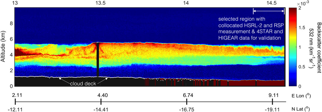
FIGURE 3. HSRL-2 aerosol backscatter at 532 nm along ER-2 flight on September 12, 2016. The white piece of line marks the temporal window from 14:25 to 14:34UTC when the HSRL-2 and RSP collocated measurements were made. The ER-2 aircraft flew a distance ∼100 km from (−18.73°N, 8.72°E) to (−19.39°N, 9.39°E) within this temporal window. A total of 50 sets of observations are identified to test the combined retrieval with a simultaneous use of RSP and HSRL-2 data.

FIGURE 4

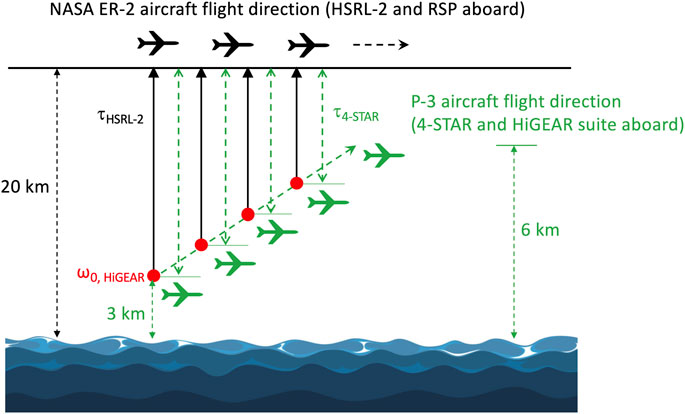
FIGURE 4. Collocation of HSRL-2, 4-STAR, and the HiGEAR suite of instrumentation in taking measurements. The column aerosol optical depth accumulated from the position of the ER-2 aircraft to the location of P-3 aircraft calculated from HSRL-2 is used to validate the retrieval and to compare to the 4-STAR reference data. The aerosol SSA derived from extinction and scattering coefficients measured by HiGEAR suite of instrumentation is used to validate the retrieved SSA. HiGEAR also provides fine and coarse mode aerosol size distributions measured by UHSAS and APS instruments at dry condition, which are compared to the retrieved size distributions at ambient condition. Approximately at the altitude from 3 to 6 km, P-3 followed the trajectory of ER-2.

The RSP instrument measures the radiance and polarimetric components Q and U in nine wavelength bands from UV (410 nm) to short-wave infrared (2,250 nm) (Cairns et al., 1999). If RSP's measurements are collocated with HSRL-2's (lat, lon) within 1 km horizontal distance, then its angular data are used for combined retrieval. For the 50 sets of observations under test, a total of 152 view angles from –39° to 25° around nadir in the wavelengths 410, 470, 550, 670, and 865 nm are used. Note that due to the yaw of the ER-2 aircraft and high altitude, RSP's view angular range is reduced to [−39°, 25°] around nadir. These measurements are within ±35° around the principal plane. The relative uncertainty is 2% for intensity and the absolute uncertainty 0.002 for DOLP. HSRL-2 is the second generation NASA Langley airborne High Spectral Resolution Lidar (Hair et al., 2008). It uses the HSRL technique (Shipley et al., 1983) to independently measure aerosol backscatter and extinction at 355 and 532 nm. While HSRL-2 products of particulate extinction, backscatter, depolarization ratio are reported at 15 m vertical resolution, the true resolution is 315 m for extinction (α_a) and 15 m for backscatter (β_a) and depolarization (δ_a) in the ORACLES campaign (Burton et al., 2018). The lidar signals that we used in this study include aerosol extinction, backscatter, and depolarization ratio. In the HSRL-2 product, the aerosol extinction at 355 and 532 nm wavelengths are under the name “355_ext” and “532_ext”, respectively. To preserve the independence of extinction data used for retrieval, we access α_a at 315 m resolution. The aerosol backscatter data at 355, 532, and 1,064 nm wavelength are under the name “355_bsc_Sa”, “532_bsc_Sa”, and “1,064_bsc_Sa”, respectively in the HSRL-2 product. Their reported values are averaged at the same resolution as extinction for lidar ratio (“S_a”) calculation. The depolarization ratios at the three lidar wavelengths are under the name “355_aer_dep”, “532_aer_dep”, and “1,064_aer_dep” for the three wavelengths in the product. In computing the error covariance matrix, an uncertainty of 17 Mm⁻¹, 5%, and 10% are assumed for α_a, β_a, and δ_a, respectively. Within the 315 m layer, optical homogeneity is assumed. Such a layer is further divided into sublayers to ensure the radiative transfer modeling accuracy.

As the assumption, two aerosol species are retrieved from the combined use of HSRL-2 and RSP observations. Each species is characterized by an independent and layer resolved set of refractive index, log-normal volumetric size distribution, and spherical particle fraction. These quantities are initialized with values in Table 1 before retrieval starts. As informed by the range of the imaginary part of the refractive index in Table 1, weakly to strongly absorbing fine mode aerosols, and non-absorbing to moderately absorbing coarse mode aerosols are assumed in retrieval. Moreover, the initial guess of the standard deviation of fine and coarse aerosol size distribution are informed by UHSAS measurements.

Retrieval Validation Against 4-STAR and HiGEAR Measurements

As the first check, a retrieval is performed using RSP and HSRL-2 collocated measurement at 14:25:10 UTC, namely the first case among the total 50 sets of collocated observations. Figure 5 displays the whole set of retrieved aerosol geophysical parameters as a function of altitude. These parameters include aerosol refractive index, volume concentration, geometric volume mean radius and logarithmic standard deviation of aerosol size distributions, and spherical particle fraction. These quantities are displayed in different panels. From the ranges of the retrieved real and imaginary parts of refractive index, the two aerosol species pre-assumed in our retrieval can be distinguished as smoke and sea salt particles.

FIGURE 5

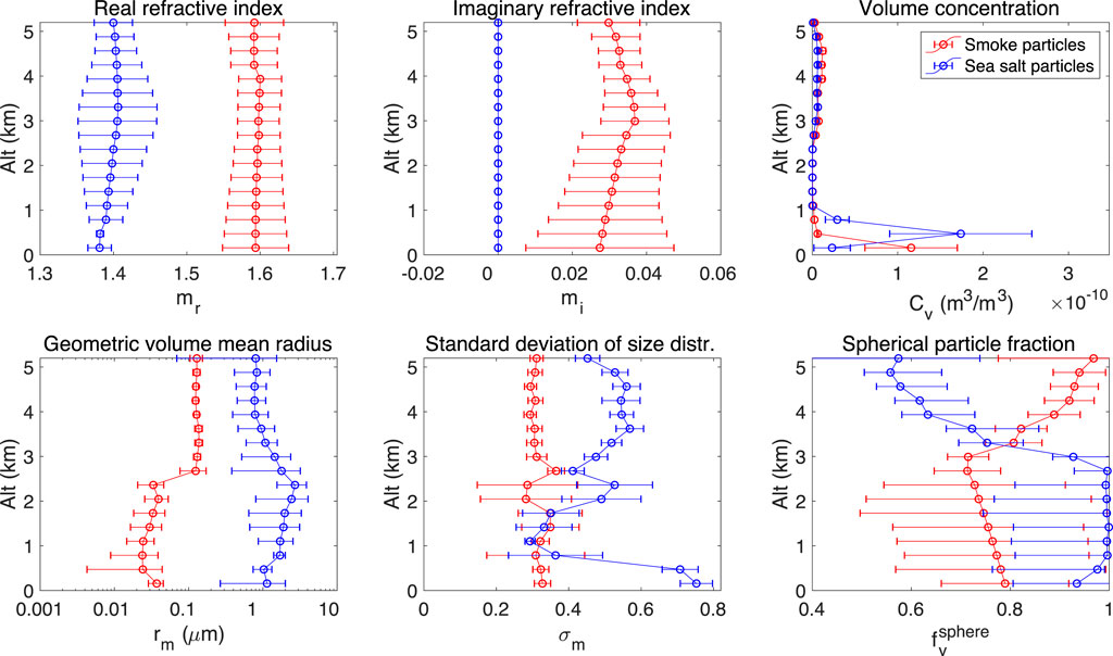
FIGURE 5. Demonstration of aerosol geophysical property retrieval using a combined set of lidar (HSRL-2) and polarimeter (RSP) observations acquired at 14:25:10UTC on September 12, 2016 during the ORACLES field campaign. Upper left panel: real part of aerosol refractive index; Upper middle panel: imaginary part of aerosol refractive index; Upper middle right panel: volume concentration (unit: m³/m³); Bottom left panel: geometric volume mean radius (unit: μm) as a function of altitude; Bottom middle panel: logarithmic standard deviation of aerosol size distribution; Bottom right panel: spherical particle fraction. The horizontal bars in all panels indicate the retrieval errors. To estimate the retrieval uncertainties, we use the relative uncertainty 2% for RSP’s intensity measurement and the absolute uncertainty 0.002 for DOLP measurement, and use the uncertainties 17 Mm⁻¹, 5%, and 10% for HSRL-2’s particulate extinction, backscatter and depolarization, respectively.

Following the transportation of biomass burning smoke particles for a long distance (e.g., >800 km) from the continent, the volumetric concentration plot shows the co-existence of smoke and sea salt particles in two regions, namely from 0 to 1 km and from 2.5 to 5.2 km. Moreover, the sea salt particles present a larger size than that of smoke particles. The spherical particle fraction for smoke and sea salt particles are ∼0.8 and >0.9, respectively, at the altitude close to the sea surface (with an retrieval uncertainty between 0.1 and 0.2). Increased nonspherical particle fraction for the sea salt particles is observed at a higher altitude from 2.5 to 5.2 km. This could be caused by crystallization as temperature, and relative humidity decreases at higher altitude. We have also noticed that the geometric mean radius of smoke particles is slightly lower in the boundary layer than in the free troposphere. In the context of the ORACLES campaign, the smoke particles in and above the boundary layer can be different in terms of their ages, transport, and microphysical properties. The smoke particles may be entrained into the PBL via large-scale re-circulation (Redemann et al., 2021) instead of directly sinking into PBL through subsidence as previously thought. Thus, the smoke aerosol properties in the PBL may be affected by their interactions with clouds or new particle formation processes. This is a likely cause of observing smaller smoke particles in the PBL than at high altitudes from the case study in Figure 5.

Calculated from the speciated aerosol abundance and intrinsic quantities displayed in Figures 5 and 6A displays the retrieved profiles of accumulated AOD (left panel) and SSA (right panel) at 532 nm (black curves), with comparison to the collocated HiGEAR measurement (red dot) at the altitude around 3 km. The retrieved AOD in the left panel of Figure 6A is accumulated AOD from TOA to different altitudes with 315 m resolution. Fairly consistent agreement between retrieved values and reference data derived from 4-STAR and HiGEAR measurements can be observed. The difference is within the estimated retrieval error for SSA and accumulated AOD. In Figure 6B, the retrieved fine mode (left panel) and coarse mode (right) aerosol size distributions (black curves) are compared to the in-situ HiGEAR measurement averaged within a vertical bin of 315 m (red curves). To compare to the number weighted aerosol size distribution measured by UHSAS and APS, the retrieved volumetric size distribution Eq. 2 needs a conversion. Specifically, the retrieved $r_m^{\left(s\right)}$ and ${\sigma }_m^{\left(s\right)}$ are converted to the geometric number mean radius $r_g^{\left(s\right)}$ and the standard deviation for sth aerosol species ${\sigma }_g^{\left(s\right)}$ by use of the following relationship (Grainger, 2017):

$r_{\text{g}}^{\left(s\right)}=r_m^{\left(s\right)}{\mathrm{e}}^{-3{\left[{\sigma }_m^{\left(s\right)}\right]}^2},(101)$

${\sigma }_g^{\left(s\right)}={\sigma }_m^{\left(s\right)}.(102)$

On such a basis, the retrieved number weighted size distribution is calculated as

$\frac{\text{d}{n}^{\left(s\right)}\left(r\right)}{\text{d}\ln r}=\frac{1}{\sqrt{2\pi }{\sigma }_g^{\left(s\right)}}\text{exp}\left[-\frac{{(\ln r-\ln r_g^{\left(s\right)})}^2}{2{\left({\sigma }_g^{\left(s\right)}\right)}^2}\right].(103)$

While UHSAS reports number concentrations of aerosols at their geometric diameters, APS reports the concentration at aerodynamic diameters of aerosols. Therefore, the APS aerodynamic particle diameter (d_ae) needs to be converted to the geometric diameter d. This is done via d = d_ae×(χ/ρ_p)^0.5, where ρ_p is aerosol density and χ is the dynamic shape parameter. Assuming all aerosols measured by APS are sea salt particles, we adopt χ = 1.08 and ρ_p = 1.8 g/cm⁻³ (Froyd et al., 2019). Then the conversion is determined as d = d_ae/1.29. By performing such a conversion, we neglect the impact of highly irregular particles on χ and assume equivalent spherical diameter for “d” which may cause bias to the estimate of χ (Reid et al., 2003). In addition, UHSAS and APS measure the number concentrations of fine and coarse mode particles in the ranges of geometric radius [0.03, 0.5] and aerodynamic radius [0.22, 8.1] μm, respectively. Apparently, the two instruments have an overlapped measurement range of geometric radius from 0.2 to 0.5 μm. Nevertheless, this range is accounted in determining $r_{\text{g}}^{\left(s\right)}$ and ${\sigma }_{\text{g}}^{\left(s\right)}$ for both fine and coarse aerosols. With these preconditions and conversions, Figure 6B compared the retrieved particle size distribution to HiGEAR’s in-situ measurement. While the difference is basically within the retrieval error estimated using the methodology described in Retrieval Error Estimate, the coarse mode aerosol size distribution is subjected to larger retrieval errors than the fine mode aerosol size distribution.

FIGURE 6

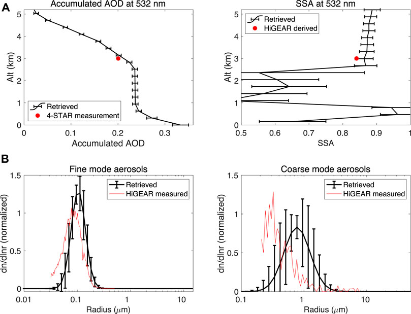
FIGURE 6. (A) Retrieved profiles of AOD (left panel) and SSA (right panel) at 532 nm (black curves), with comparison to the collocated HiGEAR measurement (red dot); (B): retrieved fine mode (left panel) and coarse mode (right panel) aerosol size distributions (black curves), with comparison to the in-situ HiGEAR measurements via UHSAS and APS (red curves). The retrieved AOD, SSA and size distribution are derived from the speciated aerosol abundance and intrinsic quantities displayed in Figure 5. Moreover, the retrieved AOD in the left panel of Figure 6A is accumulated AOD from TOA to different altitudes with 315 m resolution. The horizontal bars in all panels indicate the retrieval errors. Collocation of HiGEAR and RSP/HSRL-2 measurements was demonstrated in Figure 4. To estimate the retrieval uncertainties, the measurement uncertainties are same as those used in Figure 5.

Along with the results demonstrated in Figures 5, 6, and 7A demonstrates the retrieval fit to HSRL-2’s measurements of vertical extinction coefficient, scattering coefficients, and depolarization ratio of aerosols. The vertical mean of absolute fitting error of particulate extinction coefficient is found to be 7.6 and 8.9 Mm⁻¹ for 355 and 532 nm, respectively, for altitudes below 5.2 km, and the vertical mean of absolute fitting error of particulate backscatter is 0.16, 0.07 and 0.14 Mm⁻¹Sr⁻¹ for 355, 532 and 1,064 nm, respectively. Noticeably, the fit to the particulate backscatter of 1,064 nm at ∼1.4 km altitude has a relatively larger error. Indeed, to derive vertically resolved backscatter at 1,064 nm one needs to know the extinction at the same wavelength. Since HSRL-2 does not measure extinction at 1,064 nm directly, it is estimated from an assumed relationship with the measured lidar ratio at 532 nm. Though provided as a best guess, such an estimate may cause extra uncertainty to the 1,064 nm backscatter, which is beyond our 5% error estimate for particulate backscatter at all wavelengths. The comparison of the depolarization ratio fit to the measurements was demonstrated in the bottom panels of Figure 7A. In the altitude range from 2.5 to 5.2 km, the fitting at the 532 nm wavelength is noticeable to be beyond the measurement error. Considering that the depolarization is highly relevant to aerosol non-sphericities, such a deviation may be caused by the modeling errors with the pre-assumed aspect ratio distribution of spheroidal particles (Legrand et al., 2014). In Figure 7B, we compare the fit of aerosol lidar ratio (S_a = α_a/β_a) to the measurements. Plotted as the horizontal error bars, the measurement uncertainty with aerosol lidar ratio (ΔS_a) is derived from the uncertainties of extinction (${\sigma }_{{\alpha }_{\text{a}}}=17$ Mm⁻¹) and backscatter coefficients (${\epsilon }_{{\beta }_{\text{a}}}=5\%$) via error propagation $\Delta S_a={\alpha }_a/{\beta }_a\sqrt{{\left({\sigma }_{{\alpha }_a}/{\alpha }_a\right)}^2+{\left({\epsilon }_{{\beta }_a}\right)}^2}$. In the altitude ranges from 0 to 1 km and from 2.5 to 5.2 km where most aerosols are distributed, the fitting errors are observed to be less than 20 Sr, or less than 20% in relative sense viewing the measured lidar ratio is larger than 100 in 355 and 532 nm. Such a difference is within the measurement uncertainties of the lidar ratio indicated by the horizontal error bars.

FIGURE 7

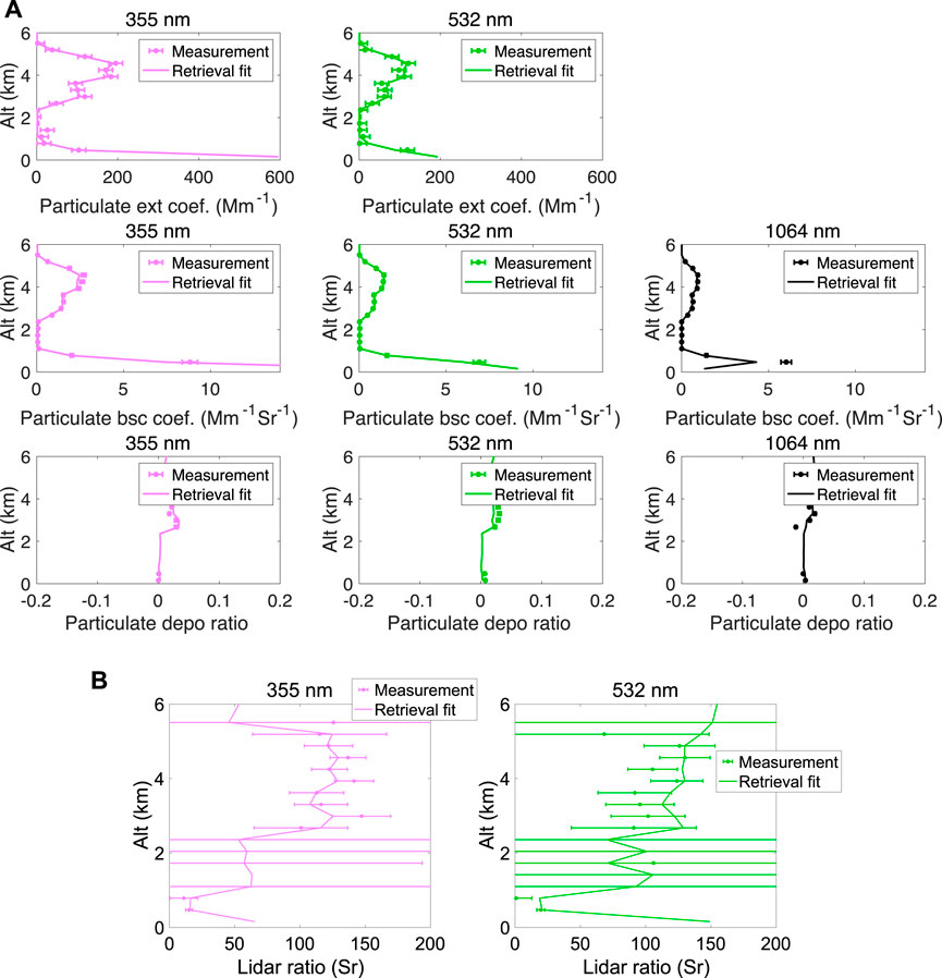
FIGURE 7. Comparison of HSRL-2 measurements with model fit using the retrieved aerosol properties displayed in Figure 6. Consistent with Figures 5 and 6, the observations were acquired at 14:25:10 UTC on September 12, 2016 during ORACLES campaign. (A) Upper panels: extinction coefficients at 355 nm (left) and 532 nm (right) as a function of altitude; Middle panels: backscatter coefficient at 355 nm (left), 532 nm (middle), and 1,064 nm (right) as a function of altitude. Bottom panels: depolarization ratio at 355 nm (left), 532 nm (middle), and 1,064 nm (right) as a function of altitude. (B) Lidar ratio at 355 nm (left) and 532 nm (right). The horizontal bars in all panels indicate the measurement uncertainties. The measurement uncertainties are same as those used in Figure 5.

The retrieved BRF and DOLP are compared to the measured data by RSP in Figure 8. The spectral mean of fitting error for BRF and DOLP is less than ∼2% and 0.003 respectively in the four bands centered at 410, 470, 670, and 865 nm. By contrast, the fitting error at 550 nm is relatively larger (∼4.5% for BRF and ∼0.007 for DOLP), which could be caused by the approximation in estimating the ozone absorption to be ∼0.03 in optical depth at 550 nm for radiance calculation, and/or due to the residue error of instrument calibration. Moreover, the fitting errors have certain angular dependence: relatively larger fitting errors can be observed when the polarimeter’s view angle gets more and more off nadir. This could be caused by the inhomogeneity in the spatial distribution of aerosols in the measurement zone, as seen from the lidar curtain in Figure 3.

FIGURE 8

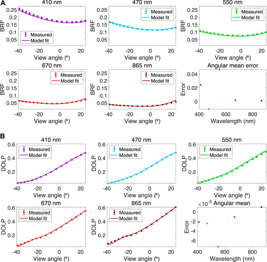
FIGURE 8. (A) Comparison of RSP radiance measurements (in BRF unit) with model fit using the retrieved aerosol properties displayed in Figure 5. Consistent with Figures 5 and 6, the observations were acquired at 14:25:10UTC on September 12, 2016 during ORACLES campaign. Comparison is made for five wavelengths from near UV (410 nm) to near-infrared (865 nm) in different panels. (B) Comparison of RSP DOLP measurements with model fits using the retrieved aerosol properties displayed in Figure 5. The vertical bars in all panels indicate the measurement uncertainties.

Following the case study demonstrated through Figures 5–8, Figure 9 gives a systematic comparison of AOD and SSA at 532 nm from all 50 sets of retrievals to the measurements by 4-STAR and HiGEAR instruments. Starting from the maximum flight altitude (6 km) of P-3 aircraft, which carries 4-STAR and HiGEAR, the accumulated AOD measured by 4-STAR is sampled at a resolution of 315 m. Plotted in red dots, comparison of retrieval to 4-STAR reference data shows the MAD to be around 0.006, which is within the AOD retrieval errors for all cases. The determinant of regression is about 0.99. As another measure of the quality of retrieved resolution in fitting observation, we also compare retrieved AOD to HSRL-2 AOD calculated from its extinction measurements. As indicated with the blue squares, most data fall very close to the 1:1 line - indicating a high quality of the agreement. Also, at the vertical resolution of 315 m, the right panel of Figure 9 shows the MAD of SSA retrievals is 0.028. Overall, the retrieved SSAs are slightly larger than HiGEAR reference data derived from its measurement of absorption and scattering coefficients. This could be due to the retrieved aerosol properties from RSP and HSRL-2’s observations are under ambient conditions, while the in-situ measurements of absorption and scattering coefficients are under dry conditions. However, seeking an exact explanation for such a difference is hard since it is within the estimated retrieval errors of SSA. Indeed, gaining an SSA retrieval accuracy of 0.028 is largely due to the constraints provided by RSP’s multiangle polarimetry, by HSRL’s direct measurement of extinction, as well as by the smoothness constraints imposed on the variation of refractive index and size distribution. The benefits of using polarimetry to constrain the retrieval of aerosol SSA has been demonstrated by multiple airborne polarimeters such as RSP (Wu et al., 2015), AirMSPI (Xu et al., 2017), AirSPEX (Hasekamp et al., 2019) and AirHARP (Puthukkudy et al., 2020). Generally, retrieval error is within ∼0.02–0.04 when the absolute error with DOLP measurement is less than ∼0.005. However, in this work, we are retrieving vertically dependent aerosol properties. Therefore, the parameter space is significantly expanded, and the polarimeter’s capability may spread increasingly thin as the number of vertical layers for retrieval to resolve increases. To mitigate this issue, extra a priori constraints regarding smooth variations of some aerosol properties are imposed, and they play a significant role in retrieval accuracy enhancement. Similar to the comparison of AOD in the left panel of Figure 9, the left and right panels of Figure 10 give a comparison of the accumulated AODs against the product of 4-STAR at 355 and 1,064 nm, respectively. The MADs of AOD at these two wavelengths are found to be 0.010 and 0.004, respectively. As a retrieval quality check, the comparison was also made to AOD calculated from HSRL-2’s extinction measurement in 355 nm. Compared to the agreement of retrieval AOD and HSRL-2 AOD in 532 nm, the agreement of the two AODs in 355 nm slightly reduces. For AOD at 1,064 nm, the difference in the retrieval and 4-STAR AODs falls beyond the range of retrieval error bars at some points. To fill the gap, we may need to further account for the uncertainties in 4-STAR AOD measurements (e.g., ∼0.01 for above-cloud AOD sampled at 500 nm and 1,020 nm according to LeBlanc et al., (2020)).

FIGURE 9

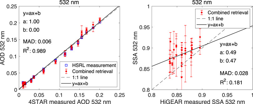
FIGURE 9. Systematic comparison of accumulated partial-column AOD and layer-effective SSA from retrieval using 50 combined sets of HSRL-2 and RSP observations to the reference measurement by 4-STAR and HiGEAR. Left panel: comparison of accumulated AOD at 532 nm against 4-STAR and HSRL-2 measurements; Right panel: comparison of SSA at 532 nm against HiGEAR reference data. Collocation of these measurements was demonstrated in Figure 4. For SSA comparison, less than 50 retrieval data points are plotted due to the screening of data for altitude above 5.2 km (too low aerosol loading). The vertical bars in all panels indicate the retrieval errors.

FIGURE 10

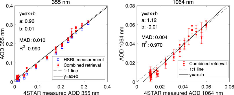
FIGURE 10. Same as the left panel of Figure 9 but the comparison against 4-STAR and HSRL-2 reference data for AOD at 355 nm, and against 4-STAR reference data for AOD at 1,064 nm. Left panel: comparison of AOD at 355 nm; Right panel: comparison of AOD at 1,064 nm. The vertical bars in all panels indicate the retrieval errors.

Figures 11 and 12 compare the effective radius and effective variance of fine and coarse mode aerosols against the reference data derived from in-situ measurements by use of the UHSAS and APS instruments aboard P-3 aircraft. We filtered out the results above 5.2 km where aerosols loading is very low so that the retrieved aerosol microphysical properties are subjected to relatively larger retrieval errors. Moreover, the UHSAS/APS measured the size-resolved number concentration are fit with the number weighted log-normal size distribution expressed in Eq. 103. Following the derivation of $r_g^{\left(s\right)}$ and ${\sigma }_g^{\left(s\right)}$ from fitting in-situ measurements, the effective radius and variance is calculated via

$r_{\text{eff}}^{\left(s\right)}=r_g^{\left(s\right)}{\mathrm{e}}^{\frac{5}{2}{\left[{\sigma }_g^{\left(s\right)}\right]}^2},(104)$

$v_{\text{eff}}^{\left(s\right)}={\mathrm{e}}^{{\left[{\sigma }_g^{\left(s\right)}\right]}^2}-1.(105)$

Comparison of fine and coarse mode aerosol effective radii and variance in the left panel of Figures 11 and 12 indicates the retrieved values are larger than their counterparts as measured by UHSAS and APS. The MADs of effective radii are around 0.012 and 0.377 μm for fine and coarse aerosols, respectively. Such a difference is basically within the estimated range of retrieval errors. MADs of effective variance are around 0.132 and 0.257 for fine and coarse aerosols, respectively. Such a deviation is beyond the range of estimated retrieval errors. However, the in-situ aerosol size measurement by HiGEAR suite of instruments has 5% (Uin 2016) and 10% (Pfeifer et al., 2016) uncertainty for fine and coarse mode aerosols, respectively. Moreover, HiGEAR measurement was carried out under dry conditions while the retrieved aerosol properties from RSP and HSRL-2’s observations were under ambient conditions. These are potential sources that can cause the difference in the estimated geometric number mean radius and standard deviation from HiGEAR measurements, which further impacts the comparison of aerosol effective radius and variance.

FIGURE 11

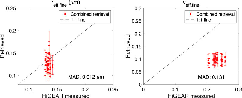
FIGURE 11. Comparison of effective radius (left panel) and variance (right panel) of fine mode aerosol size distribution. The vertical bars in all panels indicate the retrieval errors.

FIGURE 12

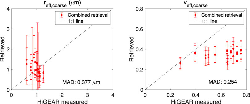
FIGURE 12. Same as Figure 11 but for coarse mode aerosol size distribution.

Summary

An optimization approach is developed to combine the use of lidar and polarimetric observations to retrieve the vertical profiles of speciated aerosol abundance and properties over the ocean. These aerosol properties include aerosol refractive index, size distribution, and spherical particle fractions. Acquired during 2016 ORACLES field campaign, the HSRL-2 measurements of extinction, backscatter and depolarization in combination with RSP measurements of radiance and DOLP are used to test the retrieval. Comparison to the accumulated AODs from TOA to different altitudes measured by 4-STAR aboard the P-3 at different altitudes (up to 6 km) shows an MAD of 0.010, 0.006, and 0.004 for 355, 532 and 1,064 nm, respectively. At the vertical resolution of 315 m, validation of SSA against the in-situ measurement by HiGEAR shows an accuracy of 0.028 for 532 nm. Comparing the retrieved effective radii of fine and coarse mode aerosols to the reference data from in-situ measurements by UHSAS and APS, we found the MADs to be around 0.012 and 0.377 μm for fine and coarse mode aerosols, respectively.

While most comparisons indicate that the differences are within the estimated retrieval errors or within measurement uncertainties of relevant quantities, it is noteworthy that we assume 1) a plane-parallel atmosphere-surface system for computing polarized radiative transfer and 2) sphere and spheroid model for computing aerosol single-scattering properties. These assumptions are subjected to errors. One error source that is particularly relevant to lidar-polarimeter combined retrieval under the context of high spatial resolution is the difference in the atmosphere viewed along nadir direction by lidar and the atmosphere viewed along oblique angles of a polarimeter. In a strict sense, combined retrieval should only use nadir polarimetric measurements, or all angular measurements but with a 3D forward RT model that accurately accounts for the spatial inhomogeneity with the atmosphere. However, the former option will reduce the benefits of multi-angular benefits in constraining while the latter option will reduce the modeling efficiency. As a trade-off between retrieval accuracy and efficiency, we use all angular measurements and retain the simplicity of assuming a plane-parallel atmosphere-surface system to perform the retrieval. Then the modeling errors are factored into the error estimates (see Retrieval Error Estimate). Nevertheless, seeking an effective way to further mitigate modeling errors while retaining the modeling efficiency is a worthwhile topic to pursue in the next stage.

Data Availability Statement

Publicly available datasets were analyzed in this study. This data can be found here: https://espoarchive.nasa.gov/archive/browse/oracles.

Author Contributions

FX formulated the inversion approach and developed the prototype codes for retrieval use. LG interfaced the retrieval with OU Supercomputing Center for Education and Research, implemented the retrieval test, and provided inputs on interpreting the results. JR, CF, WE, AS, SS, SB, XL, RF, BC and OD provided insightful discussions on the algorithm development and proper use of HSRL-2 and RSP data for retrieval test, and made editorial changes.

Conflict of Interest

The authors declare that the research was conducted in the absence of any commercial or financial relationships that could be construed as a potential conflict of interest.

Acknowledgments

The authors acknowledge support from National Aeronautics and Space Administration (NASA) for conducting the study presented in this paper. O. Dubovik acknowledges the support of the Labex CaPPA project, which is funded by the French National Research Agency under contract ANR-11-LABX-0005-01. F. Xu thanks Dr. Yongxiang Hu and Dr. Xiaomei Lu from NASA Langley Research Center for providing helpful discussions on lidar remote sensing algorithm development. The authors are grateful to the reviewers for their constructive comments on the early version of this manuscript. A majority of the computation for this project was performed at University of Oklahoma’s Supercomputing Center for Education and Research (OSCER).

References

Burton, S. P., Hair, J. W., Kahnert, M., Ferrare, R. A., Hostetler, C. A., Cook, A. L., et al. (2015). Observations of the spectral dependence of linear particle depolarization ratio of aerosols using NASA Langley airborne high spectral resolution lidar. Atmos. Chem. Phys. 15, 13453–13473. doi:10.5194/acp-15-13453-2015

CrossRef Full Text | Google Scholar

Burton, S. P., Hostetler, C. A., Cook, A. L., Hair, J. W., Seaman, S. T., Scola, S., et al. (2018). Calibration of a high spectral resolution lidar using a Michelson interferometer, with data examples from ORACLES. Appl. Optic. 57, 6061–6075. doi:10.1364/AO.57.006061

CrossRef Full Text | Google Scholar

Burton, S. P., Stamnes, S., Liu, X., Dawson, K., Chemyakin, E., Ferrare, R., et al. (2019). High spectral resolution lidar for aerosol characterization and combined lidar + polarimeter retrieval. Available at: https://www.giss.nasa.gov/staff/mmishchenko/APOLO-2/Abstracts/Burton.pdf.

Google Scholar

Cairns, B., Russell, E. E., and Travis, L. D. (1999). The research scanning polarimeter: calibration and ground-based measurements. PROC SPIE. 3754, 186. doi:10.1117/12.366329

CrossRef Full Text | Google Scholar

Chaikovsky, A., Dubovik, O., Holben, B., Bril, A., Goloub, P., Tanré, D., et al. (2016). Lidar-Radiometer Inversion Code (LIRIC) for the retrieval of vertical aerosol properties from combined lidar/radiometer data: development and distribution in EARLINET. Atmos. Meas. Tech. 9, 1181–1205. doi:10.5194/amt-9-1181-2016

CrossRef Full Text | Google Scholar

Chowdhary, J., Cairns, B., Waquet, F., Knobelspiesse, K., Ottaviani, M., Redemann, J., et al. (2012). Sensitivity of multiangle, multispectral polarimetric remote sensing over open oceans to water-leaving radiance: analyses of RSP data acquired during the MILAGRO campaign. Remote Sens. Environ. 118, 284–308. doi:10.1016/j.rse.2011.11.003

CrossRef Full Text | Google Scholar

Cox, C., and Munk, W. (1954a). Measurement of the roughness of the sea surface from photographs of the sun’s glitter. J. Opt. Soc. Am. 44, 838–850.

CrossRef Full Text | Google Scholar

Cox, C., and Munk, W. (1954b). Statistics of sea surface derived from sun glitter. J. Mar. Res. 13, l98–227.

Google Scholar

de Haan, J. F., Bosma, P. B., and Hovenier, J. W. (1987). The adding method for multiple scattering calculations of polarized light. Astron. Astrophys. 181, 371–391.

Google Scholar

Dubovik, O., Herman, M., Holdak, A., Lapyonok, T., Tanré, D., Deuzé, J. L., et al. (2011). Statistically optimized inversion algorithm for enhanced retrieval of aerosol properties from spectral multi-angle polarimetric satellite observations. Atmos. Meas. Tech. 4, 975–1018. doi:10.5194/amt-4-975-2011

CrossRef Full Text | Google Scholar

Dubovik, O., and King, M. D. (2000). A flexible inversion algorithm for retrieval of aerosol optical properties from Sun and sky radiance measurements. J. Geophys. Res. 105, 673–696. doi:10.1029/2000JD900282

CrossRef Full Text | Google Scholar

Dubovik, O., Lapyonok, T., Litvinov, P., Herman, M., Fuertes, D., Ducos, F., et al. (2014). GRASP: a versatile algorithm for characterizing the atmosphere. SPIE Newsroom 2014.

CrossRef Full Text | Google Scholar

Dubovik, O., Li, Z., Mishchenko, M. I., Tanré, D., Karol, Y., Bojkov, B., et al. (2019). Polarimetric remote sensing of atmospheric aerosols: instruments, methodologies, results, and perspectives. J. Quant. Spectrosc. Radiat. Transfer. 224, 474–511. doi:10.1016/j.jqsrt.2018.11.024

CrossRef Full Text | Google Scholar

Dubovik, O. (2004). “Optimization of numerical inversion in photopolarimetric remote sensing,” in Photopolarimetry in remote sensing. Editors G. Videen, Y. Yatskiv, and M. I. Mishchenko (Dordrecht, The Netherlands: Kluwer Academic Publishers), 65–106.

Google Scholar

Dubovik, O., Sinyuk, A., Lapyonok, T., Holben, B. N., Mishchenko, M. I., Yang, P., et al. (2006). Application of spheroid models to account for aerosol particle nonsphericity in remote sensing of desert dust. J. Geophys. Res. 111, D11208. doi:10.1029/2005JD006619

CrossRef Full Text | Google Scholar

Dunagan, S. E., Johnson, R., Zavaleta, J., Russell, P. B., Schmid, B., Flynn, C., et al. (2013). Spectrometer for sky-scanning sun-tracking atmospheric research (4STAR): instrument technology. Rem. Sens. 5, 3872–3895. doi:10.3390/rs5083872

CrossRef Full Text | Google Scholar

Espinosa, W. R., Castellanos, P., Sayer, A., Colarco, P., Kemppien, O., Nowottnick, E., et al. (2019). An exploration of joint LIDAR and multiangle polarimeter aerosol retrieval capabilities using the GRASP algorithm and OSSE data derived from the GEOS model. Available at: https://www.giss.nasa.gov/staff/mmishchenko/APOLO-2/Abstracts/Espinosa.pdf.

Google Scholar

Esposito, L. W. (1979). An “adding” algorithm for the Markov chain formalism for radiation transfer. Astrophys. J. 233, 661–663.

CrossRef Full Text | Google Scholar

Esposito, L. W., and House, L. L. (1978). Radiative transfer calculated from a Markov chain formalism. Astrophys. J. 219, 1058–1067.

CrossRef Full Text | Google Scholar

Evans, K. F., and Stephens, G. L. (1991). A new polarized atmospheric radiative transfer model. J. Quant. Spectrosc. Radiat. Transfer. 46, 413–423. doi:10.1016/0022-4073(91)90043-P

CrossRef Full Text | Google Scholar

Froyd, K. D., Murphy, D. M., Brock, C. A., Campuzano-Jost, P., Dibb, J. E., Jimenez, J.-L., et al. (2019). A new method to quantify mineral dust and other aerosol species from aircraft platforms using single-particle mass spectrometry. Atmos. Meas. Tech. 12, 6209–6239. doi:10.5194/amt-12-6209-2019

CrossRef Full Text | Google Scholar

Gao, M., Zhai, P-W., Franz, B., Hu, Y., Knobelspiesse, K., Werdell, P. J., et al. (2018). Retrieval of aerosol properties and water leaving reflectance from multi-angular polarimetric measurements over coastal waters. Optic Express. 26, 8968–8989. doi:10.1364/OE.26.008968

CrossRef Full Text | Google Scholar

GCOS (2011). Systematic observation requirements for satellite-based data products for climate; 2011 update, supplemental details to the satellite-based component of the “implementation plan for the global observing system for climate in support of the UNFCCC (2010 update). Geneva, Switzerland: WMO.

Google Scholar

Grainger, R. G. (2017). Some useful formulae for aerosol size distributions and optical properties. Available at: http://eodg.atm.ox.ac.uk/user/grainger/research/aerosols.pdf.

Google Scholar

Hair, J. W., Caldwell, L. M., Krueger, D. A., and She, C.-Y. (2001). High-spectral-resolution lidar with iodine-vapor filters: measurement of atmospheric-state and aerosol profiles. Appl. Optic. 40, 5280–5294. doi:10.1364/AO.40.005280

CrossRef Full Text | Google Scholar

Hair, J. W., Hostetler, C. A., Cook, A. L., Harper, D. B., Ferrare, R. A., Mack, T. L., et al. (2008). Airborne high spectral resolution Lidar for profiling aerosol optical properties. Appl. Optic. 47, 6734–6752. doi:10.1364/AO.47.006734

CrossRef Full Text | Google Scholar

Hansen, J. E. (1971). Multiple scattering of polarized light in planetary atmospheres. Part II. Sunlight reflected by terrestrial water clouds. J. Atmos. Sci. 28, 1400–1426. doi:10.1175/1520-0469(1971)028<1400:MSOPLI>2.0.CO;2

CrossRef Full Text | Google Scholar

Hasekamp, O., Litvinov, P., and Butz, A. (2011). Aerosol properties over the ocean from PARASOL multi-angle photopolarimetric measurements. J. Geophys. Res. 116, D14204. doi:10.1029/2010JD015469

CrossRef Full Text | Google Scholar

Hasekamp, O. P., Fu, G., Rusli, S. P., Wu, L., Noia, A. D., aan de Brugh, J., et al. (2019). Aerosol measurements by SPEXone on the NASA PACE mission: expected retrieval capabilities. J. Quant. Spectrosc. Radiat. Rransfer. 227, 170–184. doi:10.1016/j.jqsrt.2019.02.006

CrossRef Full Text | Google Scholar

Knobelspiesse, K., Cairns, B., Mishchenko, M., Chowdhary, J., Tsigaridis, K., van Diedenhoven, B., et al. (2012). Analysis of fine-mode aerosol retrieval capabilities by different passive remote sensing instrument designs. Optic Express. 20, 21457–21484. doi:10.1364/OE.20.021457

CrossRef Full Text | Google Scholar

Knobelspiesse, K., Cairns, B., Ottaviani, M., Ferrare, R., Hair, J., Hostetler, C., et al. (2011). Combined retrievals of boreal forest fire aerosol properties with a polarimeter and lidar. Atmos. Chem. Phys. 11, 7045–7067. doi:10.5194/acp-11-7045-2011

CrossRef Full Text | Google Scholar

Koepke, P. (1984). Effective reflectance of oceanic whitecaps. Appl. Optic. 23, 1816–1824.

CrossRef Full Text | Google Scholar

LeBlanc, S. E., Redemann, J., Flynn, C., Pistone, K., Kacenelenbogen, M., Segal-Rosenheimer, M., et al. (2020). Above-cloud aerosol optical depth from airborne observations in the southeast Atlantic. Atmos. Chem. Phys. 20, 1565–1590. doi:10.5194/acp-20-1565-2020

CrossRef Full Text | Google Scholar

Lee, Z. P., Hu, C., Shang, S. L., Du, K. P., Lewis, M., Arnone, R., et al. (2013). Penetration of UV-Visible solar light in the global oceans: insights from ocean color remote sensing. J. Geophys. Res. 118, 4241–4255. doi:10.1002/jgrc.20308

CrossRef Full Text | Google Scholar

Legrand, M., Dubovik, O., Lapyonok, T., and Derimian, Y. (2014). Accounting for particle non-sphericity in modeling mineral dust radiative properties in the thermal infrared. J. Quant. Spectrosc. Radiat. Transfer. 149, 219–240. doi:10.1016/j.jqsrt.2014.07.014

CrossRef Full Text | Google Scholar

Liu, X, Stamnes, S., Ferrare, R. A., Hostetler, C., Burton, S., Chemyakin, E., et al. (2016). Development of a combined lidar–polarimeter inversion algorithm for retrieving aerosol. Abstract A54E-06, AGU.

Google Scholar

Lopatin, A., Dubovik, O., Chaikovsky, A., Goloub, P., Lapyonok, T., Tanré, D., et al. (2013). Enhancement of aerosol characterization using synergy of lidar and sun-photometer coincident observations: the GARRLiC algorithm. Atmos. Meas. Tech. 6, 2065–2088. doi:10.5194/amt-6-2065-2013

CrossRef Full Text | Google Scholar

McNaughton, C. S., Clarke, A. D., Kapustin, V., Shinozuka, Y., Howell, S. G., Anderson, B. E., et al. (2009). Observations of heterogeneous reactions between Asian pollution and mineral dust over the Eastern North Pacific during INTEX-B. Atmos. Chem. Phys. 9, 8283–8308. doi:10.5194/acp-9-8283-2009

CrossRef Full Text | Google Scholar

Mishchenko, M. I., Yatskiv, Y. S., Rosenbush, V. K., and Videen, G. (2011). Polarimetric detection, characterization, and remote sensing. Cham, Switzerland: Springer.

Google Scholar

Pfeifer, S., Müller, T., Weinhold, K., Zikova, N., Martins dos Santos, S., Marinoni, A., et al. (2016). Intercomparison of 15 aerodynamic particle size spectrometers (APS 3321): uncertainties in particle sizing and number size distribution. Atmos. Meas. Tech. 9, 1545–1551. doi:10.5194/amt-9-1545-2016

CrossRef Full Text | Google Scholar

Puthukkudy, A., Martins, J. V., Remer, L. A., Xu, X., Dubovik, O., Litvinov, P., et al. (2020). Retrieval of aerosol properties from airborne hyper-angular rainbow polarimeter (AirHARP) observations during ACEPOL 2017. Atmos. Meas. Tech. 13, 5207–5236. doi:10.5194/amt-13-5207-2020

CrossRef Full Text | Google Scholar

Redemann, J., Wood, R., Zuidema, P., Doherty, S. J., Luna, B., LeBlanc, S. E., et al. (2021). An overview of the ORACLES (observations of aerosols above clouds and their interactions) project: aerosol-cloud-radiation interactions in the Southeast Atlantic basin. Atmos. Chem. Phys. 21, 1507–1563. doi:10.5194/acp-2020-449

CrossRef Full Text | Google Scholar

Reid, J. S., Jonsson, H. H., Maring, H. B., Smirnov, A., Savoie, D. L., Cliff, S. S., et al. (2003). Comparison of size and morphological measurements of coarse mode dust particles from Africa. J. Geophys. Res. 108 (D19), 8593. doi:10.1029/2002JD002485

CrossRef Full Text | Google Scholar

Remer, L. A., Knobelspiesse, K. D., Zhai, P.-W., Xu, F., Kalashnikova, O., Chowdhary, J., et al. (2019). Retrieving aerosol characteristics from the PACE mission, Part 2: multi-angle and polarimetry. Front. Environ. Sci. 7, 94. doi:10.3389/fenvs.2019.00094

CrossRef Full Text | Google Scholar

Rogers, R. R., Hair, J. W., Hostetler, C. A., Ferrare, R. A., Obland, M. D., Cook, A. L., et al. (2009). NASA LaRC airborne high spectral resolution lidar aerosol measurements during MILAGRO: observations and validation. Atmos. Chem. Phys. 9, 4811–4826. doi:10.5194/acp-9-4811-2009

CrossRef Full Text | Google Scholar

Shipley, S. T., Tracy, D. H., Eloranta, E. W., Trauger, J. T., Sroga, J. T., Roesler, F. L., et al. (1983). High spectral resolution lidar to measure optical-scattering properties of atmospheric aerosols .1. theory and Instrumentation. Appl. Optic. 22, 3716–3724. doi:10.1364/AO.22.003716

CrossRef Full Text | Google Scholar

Stamnes, S., Hostetler, C., Ferrare, R., Burton, S., Liu, X., Hair, J., et al. (2018). Simultaneous polarimeter retrievals of microphysical aerosol and ocean color parameters from the “MAPP” algorithm with comparison to high-spectral-resolution lidar aerosol and ocean products. Appl. Optic. 57, 2394–2413. doi:10.1364/AO.57.002394

CrossRef Full Text | Google Scholar

Stokes, G. G. (1862). On the intensity of the light reflected from or transmitted through a pile of plates. Proc. Roy. Soc. Lond. 11, 545–556.

Google Scholar

IPCC (2013). Climate change 2013: the physical science basis. Contribution of working group I to the fifth assessment report of the intergovernmental panel on climate change. New York, NY: Cambridge.

Google Scholar

Uin, J. (2016). Ultra-high sensitivity aerosol spectrometer (UHSAS) instrument handbook. ARM Tech. Rep. DOE/SC-ARM-TR-163, 17.

Google Scholar

van de Hulst, H. C. (1963). A new look at multiple scattering. Goddard Institute for Space Studies. Tech. Rep.NASA TM-I03044.

Google Scholar

van de Hulst, H. C. (1981). Light scattering by small particles. New York, NY: Dover.

Google Scholar

Vaughan, M. (2004). Algorithm for retrieving lidar ratios at 1064 nm fromspace-based lidar backscatter data. Proc. SPIE. 5240, 104–115. doi:10.1117/12.510770

CrossRef Full Text | Google Scholar

Weitkamp, C. (2005). LIDAR: range-resolved optical remote sensing of the atmosphere. New York, NY: Springer.

Google Scholar

Winker, D. M., Couch, R. H., and McCormick, P. (1996). An overview of LITE: NASA’s lidar in-space technology experiment. Proc. IEEE. 84, 164–180.

CrossRef Full Text | Google Scholar

Winker, D. M., Hunt, W. H., and McGill, M. J. (2007). Initial performance assessment of CALIOP. Geophys. Res. Lett. 34, L19803. doi:10.1029/2007GL030135

CrossRef Full Text | Google Scholar

Wu, L., Hasekamp, O., van Diedenhoven, B., and Cairns, B. (2015). Aerosol retrieval from multiangle, multispectral photopolarimetric measurements: importance of spectral range and angular resolution. Atmos. Meas. Tech. 8, 2625–2638. doi:10.5194/amt-8-2625-2015

CrossRef Full Text | Google Scholar

Xu, F., Davis, A. B., and Diner, D. J. (2016). Markov chain formalism for generalized radiative transfer in a plane-parallel medium, accounting for polarization. J. Quant. Spectrosc. Radiat. Transfer. 184, 14–26. doi:10.1016/j.jqsrt.2016.06.004

CrossRef Full Text | Google Scholar

Xu, F., Davis, A. B., Suniti, S. V., Martonchik, J. V., and Diner, D. J. (2012). Linearization of Markov chain formalism for vector radiative transfer in a plane-parallel atmosphere/surface system. Appl. Optic. 51, 3491–3507. doi:10.1364/AO.51.003491

CrossRef Full Text | Google Scholar

Xu, F., Davis, A. B., West, R. A., and Esposito, L. W. (2010). Markov chain formalism for polarized light transfer in plane-parallel atmospheres, with numerical comparison to the Monte Carlo method. Optic Express. 19, 946–967. doi:10.1364/OE.19.000946

CrossRef Full Text | Google Scholar

Xu, F., Davis, A. B., West, R. A., Martonchik, J. V., and Diner, D. J. (2011). Markov chain formalism for vector radiative transfer in a plane-parallel atmosphere overlying a polarizing surface. Opt. Lett. 36, 2083–2085. doi:10.1364/OL.36.002083

PubMed Abstract | CrossRef Full Text | Google Scholar

Xu, F., Diner, D. J., Dubovik, O., and Schechner, Y. (2019). A correlated multi-pixel inversion approach for aerosol remote sensing. Rem. Sens. 11, 746. doi:10.3390/rs11070746

CrossRef Full Text | Google Scholar

Xu, F., van Harten, G., Diner, D. J., Kalashnikova, O. V., Seidel, F. C., Bruegge, C. J., et al. (2017). Coupled retrieval of aerosol properties and land surface reflection using the Airborne Multiangle SpectroPolarimetric Imager. J. Geophys. Res. Atmos. 122, 7004–7026. doi:10.1002/2017JD026776

CrossRef Full Text | Google Scholar