A Comprehensive Description of Multi-Term LSM for Applying Multiple a Priori Constraints in Problems of Atmospheric Remote Sensing: GRASP Algorithm, Concept, and Applications

We describe an approach called the Multi-term Least Square Method (LSM) that has been used to develop complex aerosol inversion algorithms for a number of years and applied to retrievals of laboratory and ground-based measurements. Theoretically, it was shown how to unite the advantages of a variety of approaches and to provide transparency and flexibility in development of practically efficient retrievals. From a practical viewpoint, this approach provides a methodology for using multiple a priori constraints to atmospheric problems where rather different groups of parameters should be retrieved simultaneously. For example, Dubovik and King (J. Geophys. Res., 2000, 105, 673–696) used multi-term LSM for designing the algorithm that retrieves aerosol size distribution and spectrally dependent complex index of refraction from Sun/sky-radiometer ground-based observations. Furthermore, the significant potential of the multi-term LSM approach was demonstrated with the development of the GRASP (Generalized Retrieval of Aerosol and Surface Properties) algorithm. The GRASP algorithm is based on several generalization principles with the idea to develop a scientifically rigorous and versatile algorithm. It has significantly extended capabilities and areas of applicability and can be applied to diverse remote sensing observations. This paper also illustrates the practical applicability of GRASP and, therefore the multi-term LSM, in diverse situations.

GRASP has two main independent modules. The first module is a numerical inversion that includes general mathematical operations not related to a particular physical nature of the inverted data. Numerical inversion is implemented as a statistically optimized fitting of observations following the multi-term LSM strategy. The presentation of the GRASP numerical inversion provides a profound description of the main methodological aspects used for establishing a multi-term LSM approach that is aimed at applying multiple a priori constraints in the retrieval. The foundation of this approach uses the fundamental frameworks of the Method of Maximum Likelihood (MML) and LSM statistical estimation concepts. We discuss the asymptotical optimal properties of MML and LSM estimates in order to emphasize the importance of statistical estimation methods in remote sensing.

We also compare the multi-term LSM with other established statistical optimization approaches of numerical inversion that are constrained by a priori information, such as Bayesian concepts and the Optimal Estimation approach (Rodgers, Inverse Methods for Atmospheric Sounding: Theory and Practice, 2000). In addition, we discuss several other methodological inversion optimization aspects, including accounting for non-negativity of measured and retrieved characteristics, optimizing inversion in non-linear cases, accounting for measurement redundancy, estimating contributions of random measurement and systematic errors on the retrieval uncertainties, etc. All of these aspects are complimentary to multi-term LSM that need to be fully addressed in the development of practically efficient inversion algorithms. These methodological developments have already been applied to several remote sensing algorithms, such as the algorithm by Dubovik and King (J. Geophys. Res., 2000, 105, 673–696) that has been employed for more than two decades for operational processing of observations from AERONET ground-based Sun-sky radiometers, and the algorithm by Dubovik et al. (J. Geophys. Res., 2006, 111, D11208) developed for retrieval of aerosol particle refractive index together with size and shape distributions from full phase matrix measurements.

The second main module of GRASP is the forward model. Similarly to the numerical inversion module, it has been developed in a universal way for simulating various atmospheric remote sensing observations with high accuracy. As a result, GRASP is a highly versatile algorithm that can be applied to diverse passive and active satellite and ground-based atmospheric observations and is inherently designed for synergetic retrievals when different observations are inverted simultaneously. Depending on the input data, GRASP can retrieve detailed columnar and vertical aerosol properties and surface reflectance. Diverse approaches for modeling aerosol and surface properties together with different a priori constraints can be used in GRASP retrievals.

Thus, the GRASP package can be considered as a platform for developing, testing, and refining novel retrieval concepts and their utilization in operational processing environment. In addition, GRASP is designed as a practically efficient, transparent, and accessible community open source algorithm that can be used as an advanced tool for verifying different retrieval concepts and realizing those concepts in high-performance operational software. At present, GRASP is being adapted to reprocess the observations provided by several satellite instruments, ground-based networks, single instruments, aircraft and for various synergetic data sets that combine coordinated passive and active remote sensing observations. For example, GRASP has been adapted for operational reprocessing of observations from POLDER-1, -2, -3, MERIS, and AATSR/Envisat satellite missions. There are developments of operational retrievals of aerosol and surface properties from OLCI/Sentinel-3, Sentinel-5P, 3MI/Metop-SG, and Sentinel-4 geostationary observations. GRASP has also been used for synergetic aerosol retrievals by inverting a combination of ground-based lidar and radiometer data. GRASP has also been used for interpretation of airborne and laboratory nephelometer measurements, and it has been used for developing new approaches to derive diverse aerosol properties from ground-based direct sun and diffuse sky radiation measurements by radiometers and sky cameras.

GRASP algorithm and software organization are described in detail, and an overview of GRASP applications and data products is provided.

1 Introduction

The multi-term LSM (Least Square Method) strategy has been proposed and advocated for more than two decades in series of studies (Dubovik et al., 1995; Dubovik and King, 2000; Dubovik 2004; Dubovik et al., 2006; Dubovik et al., 2008; Dubovik et al., 2011; King and Dubovik, 2013, etc.). These realized algorithmic developments showed the multi-term LSM as fruitful methodology both for understanding the advantages of well-known approaches of constrained inversion and for constructing new practically efficient retrieval methods relying elaborated a priori constraints. The above algorithmic studies and implementations have also advanced many complimentary aspects addressing various issues and needs of successful implementation of the proposed retrieval methodology in practical applications. Specifically, the questions of implementing multi-term LSM strategy in both linear and non-linear cases, accounting for non-negativity nature of measured and retrieved characteristics, dealing with redundancy of observations, assuring consistency of multiple constraints, estimating retrieval errors, similarities and differences with other methodologies, etc. were discussed and analyzed in depth. It was shown that most of standard approaches for constraining inversion solution could be derived and optimized in the frame of multi-term LSM strategy. Moreover, this strategy is not limited to any particular application and advocated as quite universal concept for designing new practical procedures for advanced constrained inversion techniques. As a practical result of these multi-year methodological efforts a highly versatile algorithm GRASP (Generalized Retrieval of Aerosol and Surface Properties) for atmospheric remote sensing has been proposed and implemented. The description of GRASP algorithm structure and details of implementations will be used in this paper for illustrating the practical utilization of multi-term LSM approach. The GRASP development was pursuing the idea for creating the algorithm that works with diverse remote sensing applications, is convenient for application to diverse synergetic processing of the complimentary observations and well adapted for continuing evolution once used by the community. Figure 1 illustrates the concept of the algorithm. The algorithm is a useful practical tool for interpretation of actual remote sensing data and illustrates the usefulness of utilizing the multi-term LSM in diverse applications.

FIGURE 1

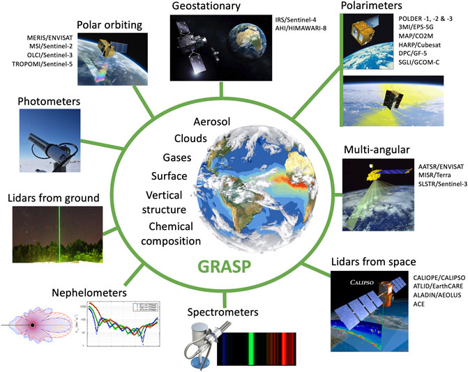
FIGURE 1. Illustration of the GRASP algorithm concept. Acknowledgment: the figure uses several images adapted from the website of NASA and ESA, from Reed et al. (2019) and also from https://www.maxpixel.net/ distributed under Creative Commons license originally authored by C. Jenkinson, B. Koenig, and R. Kokich.

The GRASP development was initiated by Dubovik et al. (2011) in the frame of the efforts on designing satellite algorithm of new generation for improving aerosol retrieval from POLDER-3/PARASOL imager over land surfaces where the high surface reflectance dwarfs the signal from aerosols. It derives simultaneously a large number of parameters characterizing aerosol and surface properties. GRASP also relies on the heritage of earlier efforts on developments for retrieving aerosol properties from the ground-based observations by AERONET network radiometers (Dubovik et al., 2000; Dubovik and King, 2000; Dubovik, 2004; King and Dubovik, 2013) and from laboratory measurements of aerosol phase matrices (Dubovik et al., 1995; Dubovik et al., 2006, etc.). All above algorithms had significant similarities and even common blocks used for mathematical inversion and observation modeling. Therefore, it has become quite logical and appealing from diverse considerations to merge these different retrievals in one single algorithm based on unified principles. Having such strategy is helpful for benefiting from historical positive experience in new retrieval developments and for developing successive strategy for evaluating and improving these unified principles and therefore for advancing the retrieval strategy in general. The overall idea of such algorithm and many specific features are aimed to address the existing challenges of modern remote sensing data interpretation (Dubovik et al., 2021). Thus, GRASP unified algorithm and software was developed as a tool applicable to many different observations that is alternative to development of several retrieval codes dedicated to interpretation of different remote sensing observations. GRASP has been developed as freely assessable software from a platform for GRASP open source code (https://www.grasp-open.com/), introductory video is available at (http://www.youtube.com/watch?v=PcDeqwDF15A). Moreover, recently GRASP-CLOUD services have been offered to remote sensing community described in details by Aspetsberger et al. (2019).

GRASP is based on several generalization principles with the idea to develop scientifically rigorous, versatile, practically efficient, transparent and accessible algorithm. Two main modules of GRASP numerical inversion and forward model are independent, can be changed separately and even fully replaced if needed for a particular application. Indeed, numerical inversion includes general mathematical operations and forward model module is developed for simulating various atmospheric remote sensing observations. Both modules are described below in details. As it will be shown many specific features in both modules can be adapted to a particular application. Following the multi-term LSM strategy the numerical inversion was implemented as a statistically optimized fitting of observations that unites the advantages of a variety of known approaches (Dubovik, 2004). For example, in aerosol retrievals, different smoothness constraints were applied simultaneously on aerosol size distributions and spectral dependencies of aerosol refractive index (see Dubovik and King, 2000; King and Dubovik, 2013). In addition, the multi-term LSM has been used for formulation of multi-pixel retrieval that implements simultaneous optimized inversion of a large group of independent observation (see Dubovik et al., 2011). This inversion scheme improves retrieval consistency by using known limitations on spatial and/or temporal variability of retrieved parameters. For example, in satellite retrieval, the horizontal pixel-to-pixel variations of aerosol and day-to-day variations of surface reflectance are enforced to be smooth by an additional set of a priori constraints. This concept is also promising for developing synergetic retrievals using observations that are not fully coincident in time or/and space as illustrated below in the paper.

The forward model simulates atmospheric radiation resulting from interaction of incident light with atmosphere and underlying surface. The aerosol model is assumed to be a mixture of several aerosol components with particles possibly having different compositions and shapes. A number of different concepts for parameterizing particle size distributions, refractive indices dependencies and shape mixtures can be used. A BRDM (Bi-directional Reflectance Distribution Matrix) that includes Bidirectional Reflectance Distribution Function (BRDF) and Bidirectional Polarization Distribution Function (BPDF) are used to account for the effects of surface reflectance, respectively (see GRASP Forward Model). The algorithm fully accounts for multiple interactions of scattered solar light with aerosol, gas and surface by means of solving radiative transfer equation. As one of the specific characteristics of GRASP retrieval, all calculations are done on-line without searching a pre-calculated look-up table. At the same timе, several different strategies based on trade-offs by increasing retrieval speed by the price of reducing completeness of retrieval have been realized for adapting GRASP for processing large amount of observations in timely manner for example as required from Near-Real-Time (NRT) processing of satellite observations. Thus, the structure of the algorithm is convenient for adapting and testing alternative routines for handling aerosol, surface, gas or multiple scattering contributions. This flexibility is convenient for adapting the forward modeling strategy to a completeness of the input information and time performance requirements. This makes GRASP uniquely adaptable both to ground-based observations, where information content is high and a very complex retrieval can be realized, and to single-view satellites, where the amount of input information is limited, and the forward modeling needs to be simplified.

GRASP is a versatile algorithm that can be applied to various passive and active remote sensing observations made from satellites, ground, aircraft or in laboratory and also to diverse combinations of those measurements. Depending on the input data, GRASP can be configured to retrieve columnar and vertical aerosol properties and surface reflectance. Specifically, GRASP is being adapted for reprocessing complex POLDER observations (Dubovik et al., 2011; Dubovik et al., 2019; Li et al., 2019). Chen et al. (2020) provide detailed description and discussion of currently available PODLER-3/GRASP aerosol products. Some demonstration of POLDER-3/GRASP retrievals are also documented in several other papers (Bovchaliuk, et al., 2013, Milinevsky et al., 2014, Kokhanovsky et al., 2015, Popp et al., 2016; Neukermans et al., 2018, Chen et al., 2018; Chen et al., 2019; Frouin et al., 2019, Remer et al., 2019, Sogacheva et al., 2020, Wei et al., 2020; Wei et al., 2021, etc.). It has been shown that using these advanced multi-angular polarimetric measurements GRASP can derive detailed aerosol information including aerosol absorption – a property that is very difficult to derive from satellite observations. This concept now has been adapted for research NRT retrieval from future 3MI/Metop-SG mission. At the same time, the application of GRASP was shown to be useful for deriving aerosol properties from single- and dual-view polar MERIS and AATSR/Envisat, OLCI/Sentinel-3, Sentinel 5P and geostationary Sentinel-4 observations, etc. Obviously, these observations contain less information and the number of parameters retrieved by GRASP is significantly lower than from polarimetric observation. Nonetheless, the base generalized approach of GRASP retrieval remains the same, i.e., from practical application point of view GRASP satellite retrievals are formally implemented in the same way for all observations:

1) The same assumptions are used everywhere, i.e., there are no location specific assumptions.

2) The same set of a priori constraints is applied globally.

3) The retrieval uses the same initial guess globally (e.g. for aerosol parameters);

4) Minimal or no post-processing used for the obtained results.

The outcome of such strategy will be discussed and illustrated below using the real results and; their validation.

GRASP can be equally applied to various ground-based observations. Since overall it inherits inversion strategy and many specific elements from the algorithm developed by (Dubovik and King, 2000; Dubovik et al., 2006, etc.) for inverting AERONET data (Holben et al., 1998) it can be naturally applied to the observations of ground-based sun/sky-radiometers. It should give very close results to AERONET operational code if applied in identical way as done in the network processing. At the same time, GRASP includes some additional features that can be of interest for obtaining some new results from ground-based radiometers. For example, GRASP can be applied to aerosol size information from direct Sun observations only (Torres et al., 2017), or it can implement simultaneous inversion of sequence of Sun and/or Sun/sky radiometric observations under a priori constraints on aerosol variability using multi-pixel approach. This will be demonstrated below. Schuster et al. (2019) used the code with Polarized Imaging Nephelometer measurements to mimic the AERONET retrieval algorithm and validated the results with simultaneous laboratory measurements of scattering, absorption, and particle size. Moreover, the GARRLiC (Generalized Aerosol Retrieval from Radiometer and Lidar Combined data) as a branch of GRASP was developed for inversion of coincident multi-spectral lidar and radiometer observations by Lopatin et al. (2013). Using this synergy, GARRLiC/GRASP retrieves improved aerosol columnar properties together with details about vertical aerosol variability including profiles of fine and coarse aerosol mode concentrations and vertical profiles of ${\omega }_{\text{0}}\left(\lambda \right)$, as will be illustrated below. GARRLiC/GRASP has been used in a number of studies and employed in routine processing within Aerosol, Clouds and Trace Gases Research Infrastructure (ACTRIS) (Tsekeri, et al., 2013; Bovchaliuk, et al., 2016; Benavent-Oltra et al., 2017; Tsekeri, et al., 2017; Román et al., 2018; Benavent-Oltra et al., 2019; Hu et al., 2019; Herreras et al., 2019; Titos et al., 2019; Konsta, et al., 2021). The evolution of the GARRLiC/GRASP branch, its applications to more complex lidar systems and more complex synergy processing is discussed by Lopatin et al. (2021). There are ongoing developments for utilization of the GRASP for processing other ground-based observations as those by sun and lunar sky cameras (Román, et al., 2017; 2021). In addition, GRASP has been adapted and extensively used for obtaining the aerosol observations from airplane and laboratory measurements by polar-nephelometer (Espinosa et al., 2017; Espinosa W. R. et al., 2019; Schuster et al., 2019). Such measurements by polar-nephelometer of angular distribution of intensity and polarization, as well as, total aerosol scattering and absorption, that are not affected by multiple scattering effects, are very useful for validating used aerosol model and overall verification of the concept of aerosol retrieval from remote sensing.

It should be noted that the main potential and advantage of unified GRASP software is that there are many different options for implementing retrieval and for generating and displaying the outputs that are developed in core software and can be used in different applications. Specifically, different approaches for modeling atmospheric radiation can be used in retrieval. For example, modeling of scattering by aerosol polydispersions can be realized using different models for parameterizing aerosol size distributions. Also, the aerosol retrieval can be set to derive optical properties of aerosol particles such as complex refractive index along with the size information as was realized by Dubovik and King (2000). Alternatively, the aerosol can be modeled as an internal or external mixture of different chemical aerosol components and the retrieval could be aimed for deriving aerosol chemical composition from the remote sensing observations. Such approach has been integrated in GRASP for both satellite and ground-based measurements, as discussed by Li et al. (2019). Similarly, different surface reflectance models can be used in GRASP retrievals. Also, different possibilities for using a priori constraints are available. Namely, the retrievals can be constrained by direct a priori estimated of unknowns, by using a priori smoothness assumptions on variability of any retrieved functions (e.g., size distributions, spectral dependencies, etc.) or by using a priori smoothness assumptions on variability of retrieved parameters in time or in space if multi-pixel approach is used, or by using all or several of these constraints simultaneously. For all the retrieved parameters and functions derived from them GRASP can provide the error estimation by calculating the elements of the covariance matrix. Also, GRASP is designed to provide the values of broadband fluxes and radiative forcing using retrieved parameters (see Derimian et al., 2016). In addition, for some situations the possibilities of estimating aerosol type, air quality (PM 2.5) and other characteristics of high practical and scientific interest have been introduced into GRASP.

The details of using different options in the retrieval and forward modeling, scientific and methodological concepts of setting up and utilization of GRASP in diverse applications are discussed the following sections in detail.

2 Theory of Multi-Term LSM Inversion

The inversion module is one the key parts of the GRASP algorithm and software. It is implemented based on rather general principles that are not directly related with any specific application. This is why, this module can be used with diverse forward models that make the GRASP concept fundamentally generalizable. It is important to note that the inversion module is based on a rather extensive and positive heritage of inversion algorithm developments for atmospheric remote sensing (Dubovik et al., 1995; Dubovik et al., 2000; Dubovik and King, 2000; Dubovik, 2004; Dubovik et al., 2006; Dubovik et al., 2008; Dubovik et al., 2011, etc.). As a result, the GRASP inversion strategy and software module has a generalized character and, at the same time, it is well tuned for interpretation of ground-based and satellite observations.

The inversion is implemented as a statistically optimized fitting of observations following the Multi-term LSM strategy that unites the advantages of a variety of approaches; it provides transparency and flexibility in algorithm development inverting passive and/or active observations and deriving several groups of unknown parameters (e.g., Dubovik, 2004, etc.). This methodology is designed to use the underlying LSM concept for building statistically optimum solution for practical situations when different observations and a priori data should be processed and interpreted together. Overall, the approach is based on the fundamental Method of Maximum Likelihood (MML). If there is a vector f^∗ composed by the measurements of physical characteristics f_j(a) depending on the vector of parameters a and this vector contains random measurement errors Δf^∗, i.e.,

${\mathit{f}}^{\ast }=\mathit{f}\left(\mathit{a}\right)+\Delta {\mathit{f}}^{\ast },$(2.0.1)

then the vector of unknowns a derived from Eq. 2.0.1 will inevitably contain some errors Δa. Here and everywhere below in the text, the vectors are denoted by lowercase italic letters in bold, while the matrices are denoted by the upper-case letters in bold. According to MML the solution â^best should result in modeled errors $\Delta f_j\ast =f_j\ast -f_j\left(\widehat{\mathit{a}}\right)$, corresponding to the most probable error realization, i.e., to the maximum of Probability Density Function (PDF):

$P\left(\Delta {\widehat{\mathit{f}}}^{\ast }\right)=P\left(\mathit{f}\left(\mathit{a}\right)-{\mathit{f}}^{\ast }\right)=P\left(\mathit{f}\left(\mathit{a}\right)|{\mathit{f}}^{\ast }\right)=\mathit{max}$(2.0.2)

where $\mathit{P}\left(\mathit{f}\left(\mathit{â}\right)\text{|}{\mathit{f}}^{\mathit{\ast }}\right)$ is the PDF of unknown parameters a conditioned on the measurements f^∗ and called the Likelihood Function. The MML is one of the strategic principles of statistical estimation that provides statistically the best solution in many senses (Edie et al., 1971). For example, under few rather general conditions (the derivatives of PDF should exist and be limited in the entire parameter space, etc.) the asymptotical error distribution (for infinite number of Δf^∗ realizations) of MML estimates â have the smallest possible variances of Δâ_i. Most of statistical properties of the MML solution remain optimum for a limited number of observations (Edie et al., 1971). Under the assumptions of a normal PDF, i.e.,

$P\left(\mathit{f}\left(\mathit{a}\right)|{\mathit{f}}^{\ast }\right)=\sim \exp \left(-\frac{1}{2}{\left(\mathit{f}\left(\mathit{a}\right)-{\mathit{f}}^{\ast }\right)}^{\mathrm{T}}{{\mathbf{C}}_f}^{-1}\left(\mathit{f}\left(\mathit{a}\right)-{\mathit{f}}^{\ast }\right)\right),$(2.0.3)

where ${\mathbf{C}}_f$ is the covariance matrix of errors Δf^∗. Based on MML, the maximum of PDF corresponds to the minimum of exponent of Eq. 2.0.3, i.e., the solution should satisfy to the so-called LSM condition:

$2\widehat{\Psi }\left(\mathit{a}\right)={\left(\mathit{f}\left(\mathit{a}\right)-{\mathit{f}}^{\ast }\right)}^{\mathrm{T}}{{\mathbf{C}}_f}^{-1}\left(\mathit{f}\left(\mathit{a}\right)-{\mathit{f}}^{\ast }\right)=\mathit{min}.$(2.0.4)

The minimum of the multi-term quadratic form $\widehat{\Psi }\left(\mathit{a}\right)$ corresponds to its extremum, i.e., to a point with zero gradient $\nabla \widehat{\Psi }\left(\mathit{a}\right)$:

$\nabla \widehat{\Psi }\left(\mathit{a}\right)=\mathit{0}.$(2.0.5)

For the general case of non-linear functions f_k(a) the solution can be found iteratively:

${\mathit{a}}^{\mathrm{p}+1}={\mathit{a}}^{\mathrm{p}}-\Delta {\mathit{a}}^{\mathrm{p}},$(2.0.6)

where Δa^p is the solution that can be found by solving the system of so-called normal equations, i.e.:

$\left({\mathbf{K}}_p^T{{\mathbf{C}}_f}^{-1}{\mathbf{K}}_p\right)\Delta {\mathit{a}}^p={\mathbf{K}}_p^T{{\mathbf{C}}_f}^{-1}\Delta {\mathit{f}}^p,$(2.0.7)

where $\Delta {\mathit{f}}^p=\mathit{f}\left({\mathit{a}}^p\right)-{\mathit{f}}^{\ast }$, and K_p is Jacobian matrix with the elements ${\left\{{\mathbf{K}}_p\right\}}_{ji}={\frac{\partial f_j\left(\mathit{a}\right)}{\partial {\mathit{a}}_{\mathit{i}}}|}_{\mathit{a}={\mathit{a}}^p}$. Then, the minimized quadratic form given by Eq. 2.0.4 has approaches a ${\chi }^2$ distribution with known the asymptotic limit (e.g., Fourgeaut and Fuchs 1967; Edie et al., 1971):

$2\Psi \left(\mathit{a}\right)=\mathit{min}\to \left(N_{\mathrm{f}}-N_{\mathrm{a}}\right),$(2.0.8)

where N_f - number of measurements and N_a - number of unknowns, i.e. numbers of elements in the vectors f^∗ and a.

2.1 Multi-Term LSM Approach for Inverting Multi-Source Data

The multi-term LSM concept is adapted in GRASP for combining information from different data sources. This approach has been formulated for implementing the flexible constrained inversion as a statistically optimized inversion of multi-source data. The concept follows the developments of Dubovik et al. (1995), Dubovik and King (2000), Dubovik et al. (2000), Dubovik (2004), Dubovik et al. (2008), and Dubovik et al. (2011). Such an approach is naturally derived from Eq 2.0.7 and allows generalizing various inversion formulas into a single formalism. The approach considers the situation when measurement vector f^∗ in Eq. 2.0.1 is obtained from different and independent “sources”, i.e., f^∗ and its covariance matrix has the following array structure:

${\mathit{f}}^{\ast }=\left(\begin{array}{c}{\mathit{f}}_1^{\ast }\\ {\mathit{f}}_2^{\ast }\\ \cdot \cdot \cdot \\ {\mathit{f}}_K^{\ast }\end{array}\right)\text{and}{\mathbf{C}}_f=\left(\begin{array}{cccc}{\mathbf{C}}_1& \mathbf{0}& \mathbf{0}& \mathbf{0}\\ \mathbf{0}& {\mathbf{C}}_2& \mathbf{0}& \mathbf{0}\\ \cdot \cdot \cdot & \cdot \cdot \cdot & \cdot \cdot \cdot & \cdot \cdot \cdot \\ \mathbf{0}& \mathbf{0}& \mathbf{0}& {\mathbf{C}}_K\end{array}\right)$(2.1.1)

where ${\left({\mathit{f}}^{\ast }\right)}^{\mathrm{T}}={\left({\mathit{f}}_1^{\ast },{\mathit{f}}_2^{\ast },\dots {\mathit{f}}_K^{\ast }\right)}^{\mathrm{T}}$ is a column vector, C_k is the covariance matrix of the k-th data set f_k^∗ and index k denotes different data sets or “sources”. This assumes that the data from the same source have similar error structures that are independent of errors in the data from other sources. For example, direct Sun and diffuse sky radiances have different magnitudes and are measured by sensors with different sensitivities, i.e., their errors should be independent (due to the different sensors) and likely have different magnitudes. In this situation, it is convenient to consider Eq. 2.0.1 as a joint system:

${\mathit{f}}_k^{\ast }={\mathit{f}}_k\left(\mathbf{a}\right)+\Delta {\mathit{f}}_k^{\ast },\left(k=\mathrm{1,2},\dots ,K\right),$(2.1.2)

where the index k denotes different data sets. It should be noted here that from the formal viewpoint, the only difference between Eq. 2.1.2 and Eq. 2.0.1 is that Eq. 2.1.2 explicitly outlines an expectation of an array structure for the covariance matrix C_f*. Such explicit demarcation of the input data makes the retrieval more transparent because the statistical optimization of the retrieval is driven by a covariance matrix of random errors. It should, be noted that Eq. 2.1.2 does not assume any relations between the different forward models f_k(a), i.e. forward models f_k(a) can be the same or different.

Thus, the joint PDF of independent data sets f₁^∗, f₂^∗, …, f_K^∗ can be obtained by the simple multiplication of the PDFs of data from all K sources:

$\mathit{P}\left(\mathit{f}\left(\mathit{a}\right)|{\mathit{f}}^{\ast }\right)=\mathit{P}\left({\mathit{f}}_1\left(\mathit{a}\right),\dots ,{\mathit{f}}_K\left(\mathit{a}\right)|{\mathit{f}}_1^{\ast },\dots ,{\mathit{f}}_K^{\ast }\right)={\displaystyle \prod _{k=1}^K\mathit{P}\left({\mathit{f}}_K\left(\mathit{a}\right)|{\mathit{f}}_k^{\ast }\right)}.$(2.1.3)

Then, under the assumptions of a normal PDF, one can write

$\mathit{P}\left(\mathit{f}\left(\mathit{a}\right)|{\mathit{f}}^{\ast }\right)={\displaystyle \prod _{k=1}^K\mathit{P}\left({\mathit{f}}_k\left(\mathit{a}\right)|{\mathit{f}}_k^{\ast }\right)}\sim \exp \left(-\frac{1}{2}{\displaystyle \sum _{k=1}^K{\left({\mathit{f}}_k\left(\mathit{a}\right)-{\mathit{f}}_k^{\ast }\right)}^{\mathrm{T}}{{\mathbf{C}}_k}^{-1}\left({\mathit{f}}_k\left(\mathit{a}\right)-{\mathit{f}}_k^{\ast }\right)}\right).$(2.1.4)

Thus, for multi-source data, the solution should correspond to minimum of K quadratic forms:

$2\widehat{\Psi }\left(\mathit{a}\right)=2{\displaystyle \sum _{k=1}^K{\widehat{\Psi }}_k\left(\mathit{a}\right)}={\displaystyle \sum _{k=1}^{{\rm K}}{\left({\mathit{f}}_k\left(\mathit{a}\right)-{\mathit{f}}_k^{\ast }\right)}^{\mathrm{T}}{{\mathbf{C}}_k}^{-1}}\left({\mathit{f}}_k\left(\mathit{a}\right)-{\mathit{f}}_k^{\ast }\right)=\mathit{min},$(2.1.5)

and for the non-linear functions f_k(a) the solution can be found iteratively as shown by Eq 2.0.6, 2.0.7, while the left and right parts of normal system of Eq. 2.0.7 can be written as a sum of terms:

$\left({\displaystyle \sum _{k=1}^K{\mathbf{K}}_{k,p}^T}{{\mathbf{C}}_k}^{–1}{\mathbf{K}}_{k,p}\right)\Delta {\mathit{a}}^p={\displaystyle \sum _{k=1}^K{\mathbf{K}}_{k,p}^T}{{\mathbf{C}}_k}^{–1}\Delta {\mathit{f}}_k^p.$(2.1.6)

where К_k,p are Jacobian matrices at p-th iteration of the functions f_k(a) in the vicinity of a^p. This is conventional LSM solution that can be easily derived for the linear f_k(a) and can also be used for the case when f_k(a) is non-linear (see, e.g., Dubovik, 2004 and discussion in Section 1.3.2 below). Similarly, the asymptotic limit of the minimized quadratic form, for most applications, can be written as:

$2\Psi \left(\mathit{a}\right)=\mathit{min}\to {\displaystyle \sum _{k=1}^K{N}_k–\mathit{n}},$(2.1.7)

where $N_K$ is a number of measurements (inputs) in the k-th data set and n is the number of retrieved unknowns (parameters). Similarly, the a priori data sets are included in the K data sets. They are statistically independent of the measurements, i.e. they have errors with a different level of accuracy uncorrelated with the remote-sensing errors.

It should be noted that in practical application it is often convenient to use weighting matrices W_k instead of covariance matrices C_k (e.g., Linnik 1962; Twomey 1977). When several data sets inverted together the use of weighting matrices add convenient transparency into approach because it makes it evident the relative contribution of the data from different data sources (e.g., Dubovik et al., 1995; Dubovik and King, 2000; Dubovik 2004, etc.). Specifically, using the weighting matrices Eq. 2.1.6 can be written as

$\left({\displaystyle \sum _{k=1}^K{\gamma }_k}{\mathbf{K}}_{k,p}^T{{\mathbf{W}}_k}^{–1}{\mathbf{K}}_{k,p}\right)\Delta {\mathit{a}}^p={\displaystyle \sum _{k=1}^K{\gamma }_k}{\mathbf{K}}_{k,p}^T{{\mathbf{W}}_k}^{–1}\Delta {\mathit{f}}_k^p.$(2.1.8)

Here the contribution of different terms in Eq. 2.1.1 are scaled by the corresponding Lagrange multipliers γ_i, defined as:

${\mathbf{W}}_i=\frac{1}{{\epsilon }_i^2}{\mathbf{C}}_i\text{and}{\gamma }_i=\frac{{\epsilon }_1^2}{{\epsilon }_i^2},$(2.1.9)

where ${\epsilon }_i^2$ is the first diagonal element of C_i, i.e., ${\epsilon }_i^2$ = {C_i}₁₁. Evidently, γ₁ = 1. As discussed by Dubovik and King (2000), Dubovik (2004), and Dubovik et al. (2011), etc., such renormalization is also convenient, because with the definition of the minimized quadratic function (or “residual”) given by Eq. 2.1.8, the measurement error ${\epsilon }_1^2$ can be estimated from the residual of the fit. Indeed, once the weighting matrices used in the solution provided by Eq. 2.1.8 minimizes quadratic with the limit depending on ${\epsilon }_1^2$:

$2{\Psi }^{\prime }\left(\mathit{a}\right)=2{\epsilon }_1^2\Psi \left(\mathit{a}\right)=\mathit{min}\to {\epsilon }_1^2\left({\displaystyle \sum _{k=1}^K{N}_k–n}\right)\text{and}$(2.1.10)

${\widehat{\epsilon }}_1^2\approx \frac{2{\Psi }^{\prime }\left({\mathit{a}}^{\mathrm{p}}\right)}{{\displaystyle {\sum }_{k=1,\dots ,K}{\mathit{N}}_{\mathit{k}}-N_{\mathbf{a}}}}.$(2.1.11)

2.1.1 A Priori Constraints in Multi-Term LSM Approach

In many practical situations, the information from measurement is not sufficient. In such situation a solution of Eq. 2.0.7 can be non-unique and inclusion of additional a priori information (constraints) becomes necessary. Multi-term LSM concept has been proposed for the integration of different types of a priori constraints in remote sensing applications (Dubovik et al., 1995; Dubovik and King 2000; Dubovik et al., 2000; Dubovik 2004; Dubovik et al., 2008; Dubovik et al., 2011). In this approach a priori estimates are considered to be “equivalent” to the measurements in the sense that the a priori data are characterized by their PDF and could be treated equivalently to the actual measurements. In this regards Eq 2.1.6–Eq 2.1.9 do not show any formal distinction between different ${\mathit{f}}_{\mathit{k}}\left(\mathbf{a}\right)$. In practice there are always two different types of data sets: direct measurements and quantified a priori knowledge about unknowns a. Therefore, the vector of the measurement ${\left({\mathit{f}}^{\ast }\right)}^{\mathrm{T}}={\left({\mathit{f}}_{\mathrm{1}}^{\ast },{\mathit{f}}_{\mathrm{2}}^{\ast },\dots {\mathit{f}}_{\mathrm{k}}^{\ast }\right)}^{\mathrm{T}}$ can be formally written as:

${\left({\mathit{f}}^{\ast }\right)}^{\mathrm{T}}={\left({\mathit{f}}_1^{\ast },{\mathit{f}}_2^{\ast },\dots ,{\mathit{f}}_k^{\ast },{\mathit{f}}_1^a,{\mathit{f}}_2^a,\dots {\mathit{f}}_n^a,\right)}^{\mathrm{T}},$(2.1.12)

where ${\mathit{f}}_i^{\ast }={\mathit{f}}_i^{\ast }\left(\mathit{a}\right)$ represent directly measured characteristics and ${\mathit{f}}_i^a={\mathit{f}}_i^a\left(\mathit{a}\right)$ represent a priori known characteristics of unknowns a. Correspondingly the right side of Eq. 2.1.3 can be formally split in two groups:

$P\left(\mathit{f}\left(\mathit{a}\right)|{\mathit{f}}^{\ast }\right)=\prod _{k=1}^{K}P\left({\mathit{f}}_k\left(\mathit{a}\right)|{\mathit{f}}_k^{\ast }\right)\prod _{n=1}^{N}P\left({\mathit{f}}_n^a\left(\mathit{a}\right)|{\mathit{f}}_n^{a,\ast }\right),$(2.1.13)

where the first group represents K sets of data obtained from actual measurements, the second group represent N sets of data ${\mathit{f}}_n^{a,\mathrm{\ast }}$ obtained from a priori knowledge.

Correspondingly, the resulting Eq. 2.1.6 can also be formally arranged to identify the contribution of measurements and a priori terms.

$\left({\displaystyle \sum _{k=1}^K{\mathbf{K}}_{k,p}^T{{\mathbf{C}}_k}^{–1}{\mathbf{K}}_{k,p}+}{\displaystyle \sum _{n=1}^N{\mathbf{K}}_{a,n,p}^T}{{\mathbf{C}}_{a,n}}^{–1}{\mathrm{K}}_{a,n,p}\right)\Delta {\mathit{a}}^p={\displaystyle \sum _{k=1}^K{\mathbf{K}}_{k,p}^T{{\mathbf{C}}_k}^{–1}\Delta {\mathit{f}}_k^{\ast ,p}}+{\displaystyle \sum _{n=1}^N{\mathbf{K}}_{a,n,p}^T{{\mathbf{C}}_{a,n}}^{–1}\Delta {\mathit{f}}_n^{a^{\ast },p}},$(2.1.14)

where two groups of the terms in left and right parts of the equation represent contributions of the set of K measured characteristics f_k(a) and the set of N a priori f_n^a(a) characteristics.

Thus, the above Multi-term approach is a simple rearranging of the base LSM formulation. At the same time, it provides the solid basis for unifying many known formulas of constrained inversion in a single formalism, as discussed by Dubovik (2004). In addition, it was shown to be practically convenient and efficient approach for developing remote sensing algorithms using diverse complimentary observations and a priori constraints. Specifically, the Multi-term approach has been successfully used in previous inversion algorithms for laboratory (Dubovik et al., 2006), ground-based (Dubovik and King, 2000; Dubovik et al., 2000; Dubovik et al., 2002), airborne (Gatebe et al., 2010), satellite observations (Dubovik et al., 2011) and in inverse modeling (Dubovik et al., 2008). All remote sensing development have been integrated into a versatile GRASP algorithm (Dubovik et al., 2014). Many of the technical details adapted in the GRASP have been previously shown and discussed. Therefore, the Sections below outline only newly introduced elements and are focused on conceptual elements of inversion as well as on user-oriented explanations of the GRASP algorithm and software utilization.

2.1.2 A Priori Constraints Used in GRASP Algorithm

The multi-term LSM concept allows flexible utilizations of nearly arbitrary a priori constraints, i.e., knowledge about any a priori known function ${\mathit{f}}_n^a\left(\mathit{a}\right)$ of unknowns a. However, only a limited number of the most popular and physically transparent a priori constraints are presently used in GRASP. At the same time, the utilization of other a priori constraints that are not included in the proposed options can also be realized upon a request.

The base configuration of GRASP proposes two types of a priori limitations: “single-pixel” and “multi-pixel” constraints. The utilization the word “pixel” in this terminology originated from interpretation of satellite images that are composed of separate pixels. Correspondingly, “single-pixel” relates to the constraints on parameters within each pixel independently, while “multi-pixel” relates to the constraints on inter-pixel spatial or temporal variability of the retrieved parameters. This classification (with the introduction of “multi-pixel” constraints) is convenient not only for the interpretation of satellite images, but it is also convenient for many other applications (laboratory and ground-based measurements) where input data can be related in time or space.

2.1.2.1 “Single-Pixel” Constraints—A Priori Constraints for Coincident and Collocated Observations

This type of constraint includes a priori information about each retrieved parameter (or characteristic in each set of measurements) that can be used absolutely independently on the measurements or as a priori knowledge in other data sets. The most common example of this type of constraint is the application of direct a priori estimates of unknowns ${\mathit{a}}^{\mathrm{\ast }}$, i.e.,

${\mathit{f}}_1^{a,\ast }={\mathit{f}}_1^{a,\ast }\left(\mathit{a}\right)+\Delta {\mathit{f}}_1^{a,\ast }\to {\mathit{a}}^{\ast }=\mathit{a}+\Delta \mathit{a},$(2.1.15)

where $\Delta \mathit{a}$ are the uncertainties of the estimates ${\mathit{a}}^{\mathrm{\ast }}$ and are generally considered to be unbiased random errors within the covariance matrix C_a∗. These constraints can be easily included in Eq. 2.1.14 by defining: ${\mathbf{K}}_{a,p}=\mathbf{1}$ - unity matrix; i.e., ${\mathbf{K}}_{a,p}^T{\mathbf{C}}_a^{–1}{\mathbf{K}}_{a,p}={\mathbf{C}}_a^{–1}$ and ${\mathbf{K}}_{a,p}^T{\mathbf{C}}_a^{\mathrm{–}1}{\mathit{f}}_{\mathrm{1}}^{\mathrm{a,\ast }}\mathrm{=}{\mathbf{C}}_a^{\mathrm{–}1}{\mathit{a}}^{\mathrm{\ast }}$. Utilization of a priori estimates ${\mathit{a}}^{\mathrm{\ast }}$ was introduced in the pioneering studies by Twomey (1963) and later evolved and discussed in detail in the Rodgers (2000) textbook on inversion.

Another common type of a priori constraint are smoothness constraints that limit the variability of retrieved functions by using a priori knowledge about limitations on derivatives of those functions. For example, a priori knowledge limits high frequency variations of continuous functions v(x), such as the aerosol size distribution, spectral dependence of the refractive index, parameters of surface reflectance, etc. From a formal point of view, the smoothness constraints are related by limited values of the derivatives, i.e., with deviations of their m-th derivative deviations from zero:

$\frac{{\partial }^{m}v\left(x\right)}{\partial x^m}\approx \mathit{0}.$(2.1.16)

For the vector of unknowns $\mathit{a=}{\left(a_1,a_2,\dots a_n\right)}^{\mathrm{T}}$ that contains the elements describing these continuous functions v(x), the knowledge on the smoothness of the retrieved function can be defined using a vector-matrix linear system (e.g., see Dubovik 2004; Dubovik et al., 2011):

${\mathit{f}}_2^{a,\ast }={\mathit{f}}_2^{a,\ast }\left(\mathit{a}\right)+\Delta {\mathit{f}}_2^{a,\ast }\to {\mathit{0}}^{\ast }={\mathbf{G}}_m\mathit{a}+{\Delta }_{\mathbf{g}}^{\ast },$(2.1.17)

where G_m is the Jacobian matrix of the matrix of the m-th derivatives, ${\mathit{0}}^{\mathrm{\ast }}$ is zero vector representing the fact that the a priori estimates of the corresponding derivatives equal to zeros. In practice, these are often approximated by matrices of the m-th finite difference estimated in point a. The errors ∆_g^∗ reflect the uncertainty in the knowledge of the deviations of y(x) from the assumed constant (m = 1), straight line (m = 2), parabola (m = 3), and so on.

Under the assumption that the ∆_g^∗ in Eq. 2.1.15 have a normal distribution with the unbiased covariance matrix ${\mathbf{C}}_{\Delta m}$, these constraints can be easily included in Eq. 2.1.14 by defining: ${\mathbf{K}}_{a,2,p}={\mathbf{G}}_m$, where ${\mathbf{G}}_m$ is Jacobian of m-th derivatives, and ${\mathit{f}}_{\mathrm{2}}^{\mathit{a}\mathrm{,\ast }}\mathrm{=}{\mathit{0}}^{\mathrm{\ast }}$. Correspondingly, the following can be written ${\mathbf{K}}_{a,2,p}^T{\mathbf{C}}_{a,2}^{-1}{\mathbf{K}}_{a,2,p}={\mathbf{G}}_m^T{\mathbf{C}}_{\Delta m}^{-1}{\mathbf{G}}_m$ and ${\mathbf{K}}_{2,p}^T{\mathbf{C}}_2^{-1}\Delta {\mathit{f}}_2^{\mathrm{a,}\ast }={\mathbf{G}}_m^T{\mathbf{C}}_{\Delta m}^{-1}\left({\mathbf{a}}^p-{\mathit{0}}^{\ast }\right)={\mathbf{G}}_m^T{\mathbf{C}}_{\Delta m}^{-1}{\mathit{a}}^p$. Utilization of such smoothness constraints was suggested by one of the first formulations of constrained inversion by Phillips (1962) and was also considered in article by Tikhonov (1963) and Tikhonov’s later studies.

Thus, for a case where only a direct a priori estimates and smoothness constraints are used, Eq. 2.1.14 can be explicitly written via weighting matrices as:

$\left({\displaystyle \sum _{k=1}^K{\gamma }_k{\mathbf{K}}_{k,p}^T{{\mathbf{W}}_k}^{–1}{\mathbf{K}}_{k,p}+{\gamma }_a{\mathbf{W}}_a^{–1}}+{\displaystyle \sum _{n=1}^N{\gamma }_n{\mathbf{\Omega }}_n}\right)\Delta {\mathit{a}}^p={\displaystyle \sum _{k=1}^{K_1}{\gamma }_k{\mathbf{K}}_{k,p}^T{{\mathbf{W}}_k}^{–1}\Delta {\mathit{f}}_k^P+{\gamma }_a{\mathbf{W}}_a^{–1}\left({\mathit{a}}^p–{\mathit{a}}^{\ast }\right)}+{\displaystyle \sum _{n=1}^N{\gamma }_n{\mathbf{\Omega }}_n{\mathit{a}}^p},$(2.1.18a)

where ${\Omega }_n$ denotes the smoothness matrices defined as

${\mathbf{G}}_m^T{\mathbf{W}}_{2,m_n}^{-1}{\mathbf{G}}_m={\mathbf{\Omega }}_{2,m_n}={\mathbf{\Omega }}_n$(2.1.18b)

Equation 2.1.18 include several smoothness constraints so that several physically independent functions can be retrieved simultaneously under different a priori smoothness constraints. For example, Dubovik and King (2000) retrieve aerosol size distribution and spectral dependence of refractive index.

Thus, Eq 2.1.18 generalize the commonly used equations of constrained inversion by Phillips (1962), Tikhonov (1963), Twomey (1975), Rodgers (1976), Twomey (1977), Rodgers (1990), and Rodgers (2000) and allows for significantly extended flexibility in practical use (Dubovik and King, 2000; Dubovik 2004, etc.)

The values of uncertainties in a priori constraints are considered to be directly comparable to uncertainties in the actual measurements and even defined in the GRASP software relatively to the measurement errors.

The definition of measurement uncertainty in GRASP code is the following:

1) Type of measurement errors:

- for each measurement data set ${\mathit{f}}_k^{\ast }$ two types of errors Δf_k^∗ can be set: relative or absolute;

2) The magnitude of the errors:

- for each data set the magnitude of the errors is defined by the standard deviation ${\epsilon }_i$ and a weighting matrix ${\mathbf{W}}_i$ (assumed as the unity matrix by default). The standard deviation is used inside of the code to calculate corresponding Lagrange multipliers ${\gamma }_i$.

Correspondingly the magnitudes of uncertainties in a priori estimates are defined in the same way as measurements. Specifically, the following “single–pixel” a priori constraints can be set in GRASP code.

“Single-pixel” a priori constraints:

1)Direct a priori estimates of unknown parameters $\mathit{a=}{\left(a_1,a_2,\dots a_n\right)}^{\mathrm{T}}$:

- for each parameter a_i an a priori value a_i^∗ can be provided with the corresponding Lagrange multipliers ${\gamma }_{a_i}$;

- it is also possible to assume a vector a^∗ of a priori estimates for all the retrieved parameters or for selected groups (e.g. parameters describing size distribution) with common Lagrange multipliers ${\gamma }_a$ and weighting matrix ${\mathbf{W}}_a$.

2) The vector a of unknows includes groups of parameters describing specific retrieved characteristics $\mathit{a=}{\left({\mathit{a}}_{sd},{\mathit{a}}_n,{\mathit{a}}_{brdf},{\mathit{a}}_h\dots \right)}^{\mathrm{T}}$, where a_sd, a_n, a_k, a_brdf, a_h are vectors containing only the parameters of size distribution, real and imaginary refractive indices and surface BRDF and aerosol vertical profile correspondingly. For each such group of parameters a_sd, a_n, a_k, a_brdf, a_h, etc. that describing describes a continuous function (e.g., a_sd) in the retrieved vector $\mathit{a=}{\left({\mathit{a}}_{sd},{\mathit{a}}_n,{\mathit{a}}_{brdf},{\mathit{a}}_h\dots \right)}^{\mathrm{T}}$ the smoothness constraints can be set by defining:

- the order m of limited derivatives (m = 0 – constant; m = 1– straight line; m = 2– parabola, etc.)

- the strength of the applied a priori smoothness constraints is defined by Lagrange multipliers ${\gamma }_n$.

The effect on the solution of applying smoothness constraints using the limitations on the derivatives can be easily illustrated. Namely, in Eq. 2.1.18 one can use only the linear system representing the a priori constraints given by Eq. 2.1.17, i.e., ${\mathit{0}}^{\ast }={\mathbf{G}}_{\text{m}}\mathit{a}+{\Delta }_{\mathbf{g}}^{\ast }$. Correspondingly, the solution of such system is provided by iterations shown by Eq. 2.1.18, where only one term is used; i.e., Eq 2.1.18 is reduced to ${\mathbf{\Omega }}_n\Delta {\mathit{a}}^p={\mathbf{\Omega }}_n{\mathit{a}}^p$. Evidently, the solution of such system is non-unique because the matrix ${\mathbf{G}}_{\text{m}}$ has a smaller number of rows (n-m – number of finite differences that approximate the corresponding derivatives) than columns (n – number of unknowns) and therefore it is evident that the matrix ${\mathbf{\Omega }}_n$ has zero determinant and the solution is non-unique, i.e., many ${\mathit{a}}^p$ could provide the equality. Correspondingly, the result strongly depends on the initial guess, i.e., iterative solutions initialized with different initial guesses would converge to different solutions. At the same time, all the solutions should satisfy the smoothness equations, i.e., each solution should be a constant for m = 1, a straight line for m = 2 and a parabola for m = 3, while the exact placement of constant, straight line or parabola depends on the initial guess. Figure 2 illustrates this consideration by showing the solutions chosen by the iterative retrieval from the same initial guess using different a priori smoothness constraints.

FIGURE 2

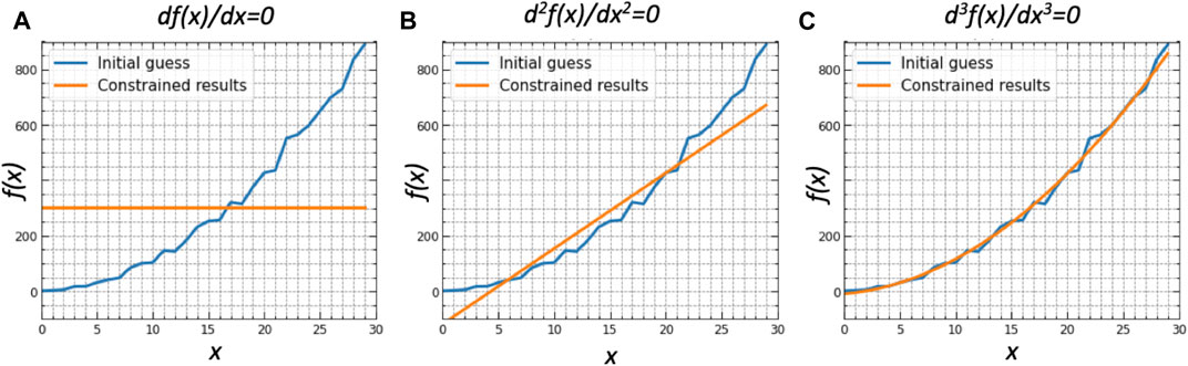
FIGURE 2. Illustration of the effect of smoothness constraints limiting derivatives of different order on the solution. The illustrations show the solutions chosen for Eq. 2.1.17 alone (no other data inverted simultaneously) by the iterative retrieval from the same initial guess under different a priori smoothness constraint. The first, second and third derivatives are a priori limited in the (A), (B), (C) correspondingly.

It should be noted, that all above “single-pixel” and “multi-pixel” (discussed in the next sections) a priori constraints implemented in the software were already actively used in practical applications and, therefore should be considered as recommended. For example, in case of “single-pixel” a priori constraints, the use of a priori estimate is often useful for the parameters or characteristics when their absolute values known from climatology or other ancillary information and the retrieved values do not expect deviate from these values and overall sensitivity of observation is not very high to these parameters. For example, such constraints are used for complex refractive index in GRASP-AOD applications (see Ground-Based Passive Observations). In satellite retrievals discussed in Satellite and Airborne Passive Observations, climatological values are often used as direct a priori estimates for some parameters of land surface reflectance. “Single-Pixel” smoothness constraints are often used for retrieval continuous function, such as aerosol size distribution, spectral dependence of complex refractive index, spectral dependence of the parameters of land surface reflectance. At the same time, the strength of a priori constraints varies significantly for different parameters. For example, smoothness constraints are much stronger for such parameters as spectral dependence of aerosol complex refractive index, then for size distribution (e.g., see Dubovik and King, 2000). Similarly the first parameter in the models of BRDF land surface reflectance is expected to have strong variation while other parameters (second, third …) describing land surface reflectance anisotropy are nearly spectrally constant (see Dubovik et al., 2011).

Finally, the practical libraries of GRASP-OPEN software provide large number of the examples of GRASP settings files that are useful examples showing how the a priori constraints in other users in realized applications.

2.1.2.2 “Multi-Pixel” Constraints—A Priori Constraints (2-D Case) for Coordinated but Non Coincident or/and Non-Collocated Observations

The GRASP “multi-pixel” fit is statistically optimized inversion that is implemented for several independent observations simultaneously (Dubovik et al., 2011), e.g., for a group of multiple satellite image pixels. Such simultaneous retrieval can be easily designed using Multi-term LSM concept defined in Eq 2.1.1–Eq 2.1.14, as described in details in paper by Dubovik et al. (2011). In “multi-pixel” fitting the state vector is composed of the state vectors from several (n) pixels:

$\mathit{a}={\left({\mathit{a}}_1,{\mathit{a}}_2,\dots ,{\mathit{a}}_{\mathrm{n}}\right)}^{\text{T}},$(2.1.19)

where each component a_i represents a state vector for a set of observations (or a “pixel” for satellite images). The observations and a priori constraints for each “pixel” are defined in exactly the same way as the “single pixel” retrieval described in Section 2.1.2.1. At the same time, implementing “multi-pixel” fitting of the data allows one to additionally use inter-pixel constraints. In fact, a priori constraints about known limited inter-pixel variability of retrieved parameters can be realized by using a priori knowledge about limitations on derivatives on time or spatial variability of parameters retrieved from observations in different pixels. Indeed, observations of different pixels provide important information about the temporal and spatial characteristics of the retrieved parameters. For example, a satellite can observe the same pixel in time and several neighboring pixels simultaneously. In principle, the variability of each physical parameter a_i can be considered as a value of a continuous function $a_i=a_j\left(x,y,z,\dots ,t\right)$. Therefore, the limitation on the variability of every parameter in time and space that can be used as additional constraints. Similar to Eq. 2.1.16, inter-pixel variability constraints are related with limited values of the derivatives, i.e., with their m-th derivative deviations from zero. At present, the time- and spatial-variation of each parameter in GRASP can be limited using the following a priori assumptions:

$\frac{{\partial }^m{a}_i\left(x,y,z,t\dots \right)}{\partial x^m}\approx 0,\frac{{\partial }^m{a}_i\left(x,y,z,t\dots \right)}{\partial y^m}\approx 0,\frac{{\partial }^m{a}_i\left(x,y,z,t\dots \right)}{\partial z^m}\approx 0,\text{and}\frac{{\partial }^m{a}_i\left(x,y,z,t\dots \right)}{\partial t^m}\approx 0,$(2.1.20)

and can be presented in matrix as similar to Eq. 2.1.17 written for a single-pixel case as:

$\{\begin{array}{c}{\mathit{f}}_2^{a,\ast }={\mathit{f}}_2^{a,\ast }\left(\mathit{a}\right)+\Delta {\mathit{f}}_2^{a,\ast }\\ {\mathit{f}}_3^{a,\ast }={\mathit{f}}_3^{a,\ast }\left(\mathit{a}\right)+\Delta {\mathit{f}}_3^{a,\ast }\\ {\mathit{f}}_4^{a,\ast }={\mathit{f}}_4^{a,\ast }\left(\mathit{a}\right)+\Delta {\mathit{f}}_4^{a,\ast }\\ {\mathit{f}}_5^{a,\ast }={\mathit{f}}_5^{a,\ast }\left(\mathit{a}\right)+\Delta {\mathit{f}}_5^{a,\ast }\end{array}\to \{\begin{array}{c}{\mathit{0}}_x^{\ast }={\mathbf{G}}_{x,m_x}\mathit{a}+{\Delta }_x^{\ast }\\ {\mathit{0}}_y^{\ast }={\mathbf{G}}_{y,m_y}\mathit{a}+{\Delta }_y^{\ast }\\ {\mathit{0}}_z^{\ast }={\mathbf{G}}_{z,m_z}\mathit{a}+{\Delta }_z^{\ast }\\ {\mathit{0}}_t^{\ast }={\mathbf{G}}_{t,m_t}\mathit{a}+{\Delta }_t^{\ast }\end{array},$(2.1.21)

where m_x, m_y, m_z and m_t are the orders of the derivatives used for limiting the time (t) and spatial (x, y, z) variation of retrieved parameters. These orders can be different for each dimension x, y, z and t.

Then, the solution for the multi-pixel fitting equivalent of Eq. 2.1.18 (written for a single-pixel case) can be presented as:

$\left(\begin{array}{cccc}{\mathbf{A}}_{1,p}& \mathbf{0}& \dots & \mathbf{0}\\ \mathbf{0}& {\mathbf{A}}_{2,p}& \dots & \mathbf{0}\\ \dots & \dots & \dots & \dots \\ \mathbf{0}& \mathbf{0}& \dots & {\mathbf{A}}_{N,p}\end{array}+{\mathbf{\Omega }}_{\text{inter}}\right)\Delta {\mathit{a}}^P=\left(\begin{array}{c}\nabla {\Psi }_1\left({\mathit{a}}_1^P\right)\\ \nabla {\Psi }_2\left({\mathit{a}}_2^P\right)\\ \dots \\ \nabla {\Psi }_N\left({\mathit{a}}_N^P\right)\end{array}\right)+{\mathbf{\Omega }}_{\text{inter}}{\mathit{a}}^P,$(2.1.22)

where ${\mathbf{A}}_{i,p}$ and $\nabla {\Psi }_i\left({\mathbf{a}}_i^P\right)$ refer to the left and right parts of Eq. 2.1.8 defined for i-th single pixel, so that Eq. 2.1.8 can be denoted compactly as ${\mathbf{A}}_{i,p}\Delta {\mathit{a}}_i^P\mathrm{=}\nabla {\Psi }_i\left({\mathit{a}}_i^P\right)$. The matrix ${\mathbf{\Omega }}_{\text{inter}}$ of multi-pixel constraints is defined via smoothness matrices for the spatial and temporal variability of each retrieved parameter as:

${\mathbf{\Omega }}_{\text{inter}}={\gamma }_x{\mathbf{\Omega }}_{x,m_x}+{\gamma }_y{\mathbf{\Omega }}_{y,m_y}+{\gamma }_z{\mathbf{\Omega }}_{z,m_z}+{\gamma }_t{\mathbf{\Omega }}_{t,m_t}.$(2.1.23)

The detailed description of multi-pixel constraints and their application is provided in the paper by Dubovik et al. (2011). Specifically, Dubovik et al. (2011) provide explicit expressions for ${\mathbf{\Omega }}_{x,m_x}$, ${\mathbf{\Omega }}_{y,m_y}$and ${\mathbf{\Omega }}_{t,m_t}$, as well as corresponding Lagrange multipliers ${\gamma }_x$, ${\gamma }_y$ and ${\gamma }_t$. The equations are fully implemented in the GRASP code. The vertical multi-pixel constraints defined by ${\mathbf{\Omega }}_{z,m_z}$ and ${\gamma }_z$ that appear logically in general Eq 2.1.20–Eq 2.1.23 are not yet implemented in a similar way as is done for horizontal and temporal constraints, because in practice there are almost no fully independent vertical observations. Instead, as was discussed in a previous Section, the a priori limitations on vertical variability are included as a part of single-pixel a priori constraints that seem to address most needs in practical applications (Lopatin et al., 2013; Lopatin et al., 2021). The illustrations of a priori constraint on vertical variability are discussed in Multi-Term LSM: Retrieval Practice Using GRASP. It should be noted that the rather complex and explicit expressions provided by Dubovik et al. (2011) are of primary interest for methodological analysis. At the same, the implementation of vertical or any other multi-pixel constraints in practical algorithms can be efficiently realized in computer routines using conceptual Eq 2.1.20–Eq 2.1.23 without using explicit visualization of the final equations.

Thus, the following “multi-pixel” a priori constraints can be set in GRASP code.

“Multi-pixel” a priori constraints:

1) For each single parameter a_i, variability along coordinate x can be limited by applying a priori constraints on the derivatives of a_i = a_i(x). For example, in satellite retrievals, the coordinate x relates with latitudinal variability. The smoothness constraints on a_i = a_i(x) can be set by defining:

- order m of limited derivatives [m = 0 – a_i = a_i(x) is close to a constant; m = 1– a_i = a_i(x) is close to a straight line; m = 2– a_i = a_i(x) is close to a parabola, etc.]

- the strength of applied a priori smoothness constraints is defined by Lagrange multipliers ${\gamma }_{x,i}$.

2) For each single parameter a_i a priori constraints on variability along coordinate y, i.e., a_i = a_i(y) can be limited. For example, in satellite retrievals, the coordinate y relates with longitudinal variability. The smoothness constraints on a_i = a_i(y) can be set by defining:

- order m of limited derivatives [m = 0 – a_i = a_i(y) is close to a constant; m = 1– a_i = a_i(y) is close to a straight line; m = 2– a_i = a_i(y) is close to a parabola, etc.]

- the strength of applied a priori smoothness constraints is defined by Lagrange multipliers ${\gamma }_{y,i}$.

3) For each single parameter a_i a priori constraints on time variability, i.e., a_i = a_i(t) can be limited. The smoothness constraints on a_i = a_i(t) can be set by defining:

- order m of limited derivatives [m = 0 – a_i = a_i(t) is close to a constant; m = 1– a_i = a_i(t) is close to a straight line; m = 2– a_i = a_i(y) is close to a parabola, etc.]

- the strength of applied a priori smoothness constraints is defined by Lagrange multipliers ${\gamma }_{t,i}$.

For the parameters with multi-dimensional variability a_i = a_i(x,y,t) the above constraints can be applied simultaneously.

For example, aerosol concentrations, values of refractive index, non-spherical fraction and any parameter used for the description of surface reflectance BRDF and BPDF can be considered as characteristics a_i = a_i(x,y,t) that change horizontally and in time. In case of applying multi-pixel constraints on the retrieved multi-dimensional function a_i = a_i(x,y,t), the smoothness constraints would force the projection of the solution at each coordinates x, y or t to take a from close to a constant, a straight line or a parabola depending which of corresponding partial derivatives $\frac{{\partial }^m{\mathit{a}}_i\left(x,y,t\right)}{\partial x^m}$, $\frac{{\partial }^m{\mathit{a}}_i\left(x,y,t\right)}{\partial y^m}$ or $\frac{{\partial }^m{\mathit{a}}_i\left(x,y,t\right)}{\partial t^m}$ with respect to x, y or t are assumed to be close to zero. Therefore limiting several different partial derivatives will force a_i(x,y,t) to the corresponding 3D surface.

Figure 3 illustrates the application of multi-pixel constraints in 2D. Similarly to the single-pixel case shown in Figure 2, one can use only reduced linear system Eq. 2.1.22 using terms representing multi-pixel a priori constraints. Evidently, the solution of such system is non-unique because the matrix in the left part of Eq. 2.1.22 is degenerated (it has smaller number of rows than columns), and the results will strongly depend on the initial guess, i.e., iterative solutions initialized with different initial guesses would converge to different solutions. Situations with a priori constraints limiting different partial derivatives are shown in Figure 3. One can see that the resulting solutions are always converge to smooth surfaces with projection on the axis x or y represented a constant, a straight line or a parabola depending which of corresponding partial derivatives in respect to coordinate x or y are limited.

FIGURE 3

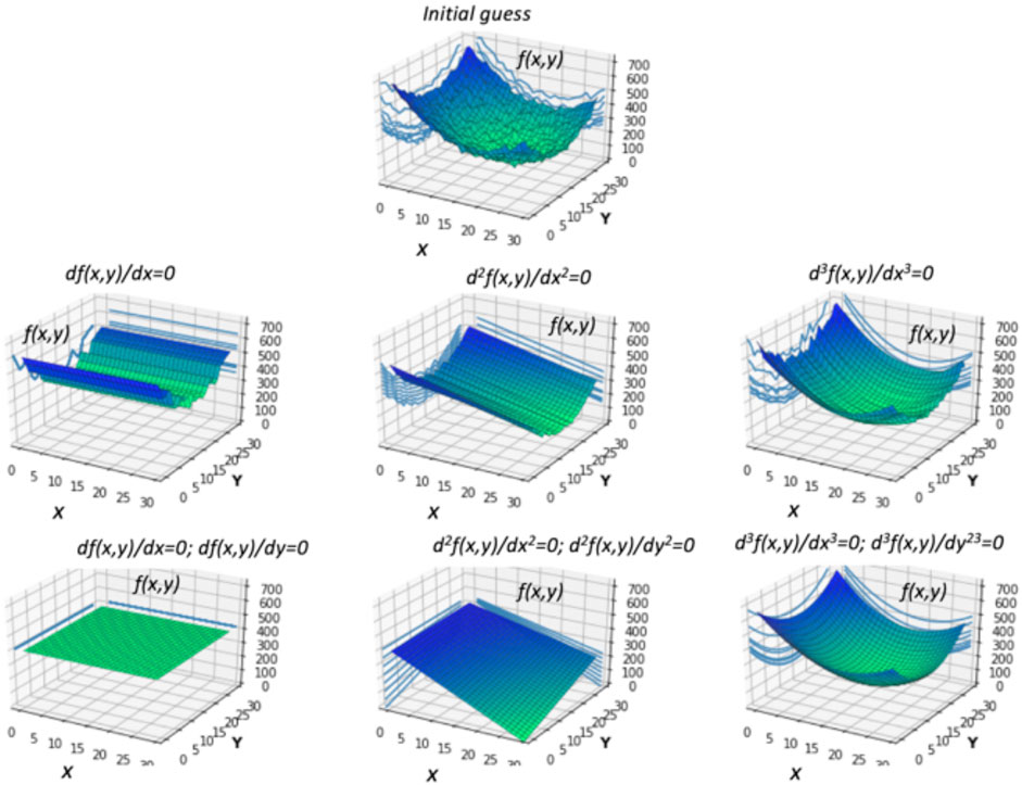
FIGURE 3. Illustration of the effect from multi-pixel smoothness constraints (2-D case). The illustrations show the solutions chosen for Eq. 2.1.2 alone (no other data inverted simultaneously) by the iterative retrieval from the same initial guess under different a priori smoothness constraint. Each panel corresponds to different set of a priori limited derivatives that shown by equation on the top of each panel.

In practical applications “multi-pixel” constraints were introduce and proven to be efficient in satellite applications. Specifically, in GRASP simultaneous retrievals of land surface and aerosol form satellite observations (see Satellite and Airborne Passive Observations, the “multi-pixel” smoothness constraints were applied to limit temporal variability for retrieved values of land reflectance and spatial variability for retrieved values of aerosol parameters (see Dubovik et al., 2011). Utilization of temporal “multi-pixel” constraints is also was shown for diverse synergy application (see discussion in Ground-Based Active Observation and Synergy With Passive Observations and Synergetic Retrievals and Other Diverse GRASP Applications). For example, Lopatin et al. (2021) used the “multi-pixel” smoothness constraints on temporal variability of aerosol parameters in simultaneous inversion of the different ground-based observations, that were obtained in the same place but not at the same time. In such approach, the “multi-pixel” smoothness constraints helped to significantly enrich the aerosol characterization.

It should be noted that, in principle, the choice of possible multi-pixel constraints is not limited to the set of constraint possibilities listed above or already realized in the software. For example, the a priori limitations can be expected for higher order or mixed partial derivatives:

$\frac{{\partial }^{\left(k_1+k_2+k_1+k_2\right)}{a}_i\left(x,y,z,t\right)}{\partial x^{k_1}\partial y^{k_2}\partial z^{k_3}\partial t^{k_4}}\approx 0.$(2.1.24)

Also, the derivatives may also have non-zero average trends which could also be useful practical constraints. Explicit derivation of the matrices ${\mathbf{\Omega }}_{\text{inter}}$, as well as understanding and visual interpretation of a priori constraints on the partial derivatives shown by Eq. 2.1.24 can be quite challenging for mixed partial derivatives of high order in N-D cases. At the same time, handling these cases using computer routines in inversion algorithms is rather straightforward. In addition, as emphasized by Dubovik et al. (2011), the matrices ${\mathbf{\Omega }}_{\text{inter}}$ are very sparse, therefore solving an apparently large matrix system of Eq. 2.1.22 can be efficiently achieved using standard numerical solvers developed for sparse systems.

In addition, Xu et al. (2019) proposed to integrate some elements of Principal Component (PC) analysis into the multi-pixel formalism. In this approach the vector of unknowns is represented via expansion using PC basis and the actual PC components and the coefficients are sought as a part of the solution. This approach allows reduction of the solution of dimensionality, decrease of calculation time and other potentially interesting solution optimizations.

All above features are considered for integration in the future evolution of GRASP.

2.1.3 Comparison With Bayesian Strategy and Optimal Estimation Approach

As discussed above, in a contrast with original approaches of constrained inversion originated by Phillips (1962), Tikhonov (1963), Twomey (1975), and Twomey (1977) the Multi-term LSM is fully based on statistical estimation methodology that suggests use of MML and LSM as the most practically efficient approach. In this regard, Multi-term LSM approach is fundamentally similar to conventional Bayesian approach used in Optimal Estimation (OE) algorithms (Rodgers 2000). At the same time, Multi-term LSM has some distinct and practically useful differences with OE approach that will be discussed below. Specifically, OE is absolutely equal to a particular case of Multi-term LSM when only direct a priori estimates are used as constraints, meanwhile the Multi-term LSM approach allows rather straightforward application of much more refined a priori constraints.

In probability theory and statistics, Bayes theorem describes the probability of an event, based on a prior knowledge of conditions that might be related to the event (e.g., Idie et al., 1971). In a similar way, any retrieval can be considered as a modification of prior knowledge about unknowns by adding information from indirect measurements f^∗(a). Such vision can be expressed mathematically using MML formalism. Namely, in situation when available a priori information can as expressed as a priori estimates a^∗ statistically independent of the measurements f^∗, the a priori estimates a^∗ can be described by Likelihood Function i.e., PDF function P(a|a^∗) that is independent of the Likelihood Function of the measurements P(f(a)|f^∗). Then, correspondingly the Likelihood Function written if both a priori estimates a^∗ and measurements f^∗ are available as a joint PDF P(a|f^∗, a^∗) can be presented as the product of P(a|a^∗) and P(f(a)|f^∗):

$P\left(\mathit{a}|{\mathit{f}}^{\ast },{\mathit{a}}^{\ast }\right)=P\left(\mathit{f}\left(\mathit{a}\right)|{\mathit{f}}^{\ast }\right)P\left(\mathit{a}|{\mathit{a}}^{\ast }\right).$(2.1.25)

Correspondingly, the MML for such a situation can be written as follows:

$P\left(\mathit{a}|{\mathit{f}}^{\ast },{\mathit{a}}^{\ast }\right)=P\left(\mathit{f}\left(\mathit{a}\right)|{\mathit{f}}^{\ast }\right)P\left(\mathit{a}|{\mathit{a}}^{\ast }\right)=\mathit{max}.$(2.1.26)

In most practical cases, it is reasonable to assume that there is some a priori knowledge a^∗ about unknowns a (even if only quite uncertain). Following such logic, Eq. 2.1.25 can be considered as a rather basic MML formulation as suggested by studies of Rodgers (2000) where it is also called the OE technique. In the simplest linear case, the OE solution corresponds to the solution of the following linear system:

$\left({\mathbf{K}}^T{\mathbf{C}}^{-1}\mathbf{K}+{\mathbf{C}}_a^{-1}\right)\mathit{a}={\mathbf{K}}^T{\mathbf{C}}^{-1}{\mathit{f}}^{\ast }+{\mathbf{C}}_a^{-1}{\mathit{a}}^{\ast }.$(2.1.27)

This OE technique is rather popular for designing linear optimized estimators for constraint inversion in remote sensing applications and it is often considered as a universal approach for integrating a priori constraints in the retrieval. However, in this regard, Multi-term LSM can propose a somewhat different view on the definition of a priori constraints that can be more convenient in some practical situations. Indeed, the Multi-term LSM Eq. 2.1.13 can be formally considered as an equivalent of Bayesian or OE formulations. Namely, the first and second terms on the right-hand side of Eq. 2.1.13 become:

$P\left(\mathit{f}\left(\mathit{a}\right)|{\mathit{f}}^{\ast }\right)={\displaystyle \prod _{k=1}^{K}P\left({\mathit{f}}_k\left(\mathit{a}\right)|{\mathit{f}}_k^{\ast }\right)}P\left(\mathit{a}|{\mathit{a}}^{\ast }\right),$(2.1.28)

where PDF of a^∗ is defined as

$P\left(\mathit{a}|{\mathit{a}}^{\ast }\right)={\displaystyle \prod _{n=1}^{N}P\left({\mathit{f}}_n^a\left(\mathit{a}\right)|{\mathit{f}}_n^{a,\ast }\right)}$(2.1.29)

For the cases where all PDFs are normal functions, the PDF $P\left(\mathit{a}|{\mathit{a}}^{\ast }\right)$ on the left side can be described only by the a^∗ covariance matrix C_a, while the right side is a product of several PDFs, each of them given for a different function ${\mathit{f}}_n^a\left(\mathit{a}\right)$ and is defined by the mean vector ${\mathit{f}}_n^{a,\mathrm{\ast }}$ and its covariance matrix ${\mathbf{C}}_a$. Correspondingly, for many practical applications, using Eq. 2.1.26 directly and finding the a^∗ covariance matrix C_a directly is not easy and even nearly infeasible. In this regard, a Multi-term LSM equation that considers an a priori PDF as a product of several different PDFs of a priori constraints is significantly more convenient for a number of practical situations. For example, Eq. 2.1.17 that was quite naturally defined above in the frame of Multi-term LSM can be obtained from optimum estimation Bayesian Eq. 2.1.25 by assuming the following a^∗ and C_a:

${\mathit{a}}^{\ast }={\left({\gamma }_a{\mathbf{W}}_a^{-1}+{\displaystyle \sum _{n=1}^{K_2}{\gamma }_n{\mathbf{\Omega }}_n}\right)}^{-1}{\gamma }_a{\mathbf{W}}_a^{-1}\left({\mathit{a}}^p-{\mathit{a}}^{\ast }\right)$(2.1.30)

and

${\mathbf{C}}_a={\epsilon }_1^2{\left({\gamma }_a{\mathbf{W}}_a^{-1}+{\displaystyle \sum _{n=1}^{K_2}{\gamma }_n{\mathbf{\Omega }}_n}\right)}^{-1}$(2.1.31)

respectively. Indeed, Eq. 2.1.28 are exactly the two key terms of Multi-term LSM expression introduced in the form of Eq. 2.1.13. Obviously, that such a^∗ and C_a can only be constructed using considerations of P(a | a^∗) and a product of many PDFs as shown in Eq 2.1.28, 2.1.29. Constructing such a^∗ and C_a could probably be useful in some situations, but generally is not necessary and often may even be impossible. For example, even the one of the simplest pioneering Phillips formulas written for the linear case:

$\left({\mathbf{K}}^T{{\mathbf{C}}_f}^{-1}\mathbf{K}+{\mathbf{\Omega }}_m\right)\mathit{a}={\mathbf{K}}^T{{\mathbf{C}}_f}^{-1}{\mathit{f}}^{\ast },$(2.1.32)

Can be derived from OE Bayesian Eq. 2.1.27 assuming a^∗ and C_a as:

${\mathit{a}}^{\ast }={\mathit{0}}^{\ast }\text{and}{\mathbf{C}}_a={\mathbf{\Omega }}_m^{-1}.$(2.1.33)

However, ${\mathbf{\Omega }}_m$ is a smoothness matrix (generally defined as ${\mathbf{\Omega }}_m={\mathbf{G}}_m^T{\mathbf{G}}_m$, e.g. Dubovik, 2004) that has det = 0, and therefore defining matrix ${\mathbf{C}}_a$ explicitly as given in Eq 2.1.30, 2.1.31 is an ambiguous and unachievable task. Evidently, more complex Multi-term LSM based equations such as Eq 2.1.18, 2.1.22 can also be presented in the OE form, however the derivations of those equations in the first place from ОЕ would not be feasible.

Finally, we would like to note the substantial conceptual difference between the Multi-term LSM approach and the OE approach. Indeed, the main idea of the multi-term LSM concept is the consideration that a priori estimates are equivalent to the measurements. In other words it is expected that a priori data can be characterized by their PDF and be treated equivalently to actual measurements. This is a different premise than the main idea of the Bayesian statistics approach, which assumes that the developer should always utilize a priori information about the entire solution before attempting the retrieval. Thus, this Bayesian assumption implicitly suggests having an a priori estimate for the entire unknown state vector as a starting point of developing the retrieval algorithm. With that in mind, the developer may feel a necessity to use at least some values as a priori estimates; for example, using his/her best guess about the possible solution even without having full justification for using these estimates. As a result, if no objective link of the assumed a priori information has been established, the Bayesian approach becomes vulnerable to subjective assumptions of the developer (which somewhat contradicts to the principle of scientific objectivity). Thus, in spite the fundamental mathematical equivalence of Multi-term LSM and OE, the differences in the base concepts may have essential influence on forming specific methodological guidelines that may lead significantly different practical recommendations.

It is interesting that from a historical prospective, Ronald Fisher was among the opponents of the Bayesian statistics and promoted development of MML as an alternative strategy (see Fisher, 1956; Agresti and Hitchcock, 2005). Fatefully, the highly popular OE approach promoted by the textbook Rodgers (2000) is often considered as an equivalent of MML by remote sensing community (especially by inexperienced readers taking the text book as introductory coarse in retrieval methodology), and it somewhat promotes the Bayesian ideas.

2.2 Further Aspects of Inversion Optimization

The optimality of MML and LSM concept is a key methodological aspect used for realizing numerical inversion in GRASP. In this respect, it is necessary to remember that this optimality can be achieved under certain conditions that need to be respected; otherwise applying the MML and LSM concept may lead to unsatisfactory results.

2.2.1 Logarithmic Transformation as Rigorous Approach to Account for Non-Negativity of Measured and Retrieved Positively Defined Parameters

One of the situations where this aspect requires specific attention relates to securing the positive solutions in the retrieval of non-negative characteristics. Historically, the straightforward use of LSM-based linear constrained inversion could generate negative values for physically non-negative characteristics in some applications, and this created contradicting situations wherein empirical, largely intuitive algorithms (Chahine 1968; Twomey 1975) performed better than algorithms based on rigorous principles of statistical optimization. Such results reduce the trust and interest of the inverse algorithm developer community in studying the rather complex statistical estimation formalism and utilizing it in practical applications. At the same time, as was discussed by Dubovik and King (2000) and Dubovik (2004), after some adjustment of hypothesis about error statistic and correct application of the concept, the MML and LSM provide very fruitful solution recipes for such situations.

Specifically, as suggested by Dubovik et al. (1995), Dubovik and King (2000) and Dubovik (2004) the non-negativity constraints can be included in the statistical estimation concept by applying lognormal noise assumption in the retrieval optimization. This assumption of lognormal noise (instead of conventional normal noise) leads to implementing inversions in logarithmic space, i.e., to employing a logarithmic transformation of the forward model. Retrieval of logarithms of a physical characteristic (instead of absolute values) is an obvious way to avoid negative values for positively defined characteristics. However, the literature devoted to inversion techniques tends to consider this apparently useful tactic as an artificial trick rather than a scientific approach to optimize solutions.

Such above misconception is probably caused by the fact that the pioneering efforts on inversion optimization by Phillips (1962), Tikhonov (1963), Twomey (1963) and many of later theoretical considerations (e.g., Hansen, 1992) were devoted to solving the Fredholm integral equation of the first kind, i.e., a system of linear equations produced by a quadrature. Examples include the retrieval of aerosol size distribution (King et al., 1978) or temperature profile of the atmosphere (Rodgers, 1976) by inverting spectral dependence of optical thickness. Considering optical thickness as a function of the logarithm of the aerosol concentrations or temperature profile requires replacing initially linear equation f = K a by nonlinear one $f_j=f_j\left(\ln a_i\right)$. On the face of it, such a transformation of linear problems to non-linear ones is not enthusiastically accepted by scientific community as an optimization. On the other hand, in cases when a forward model is a nonlinear function of the retrieved parameters (e.g., atmospheric remote sensing in cases when multiple scattering effects are significant), the retrieval of logarithms is more easiily accepted as a logical approach. Besides, non-linear Chahine-like iterative methods where proven to be efficient for inverting linear systems while Dubovik et al. (1995) and Dubovik and King (2000) have shown that under some assumptions these methods are equivalent to LSM formulated for logarithms.

Rigorous statistical considerations also reveal some limitations of applying Gaussian function for modeling errors in the measurement of positively defined characteristics. Indeed, the curve of the normal distribution is symmetrical and therefore the assumption of a normal PDF is equivalent to the assumption of the principal possibility of obtaining negative results even in the case of physically non-negative values. For such non-negative characteristics as intensities, fluxes, etc., the choice of the log-normal distribution for describing the measurement noise seems to be more correct due to the following considerations:

1) log-normally distributed values are positively-defined;

2) there is a number of theoretical and experimental reasons showing that for positively defined characteristics the log-normal curve (multiplicative errors) is the best for modeling random deviations in non-negative values [see the discussion of statistical experiments in the textbook of Tarantola (1987)].

In addition, from the practical viewpoint, using the lognormal PDF for noise optimization does not require any revision of normal concepts and can be implemented by simple transformation of the problem to the space of normally distributed logarithms. Therefore, there is a clear basis for considering log-normal PDF for measurements of fundamentally non-negative characteristics f (such as intensities, for example). Correspondingly, logarithmical transformation can be applied to the initial system of equations, i.e.,:

${\mathit{f}}^{\ast }=\mathit{f}\left(\mathit{a}\right)+\Delta {\mathit{f}}^{\ast }\to \ln {\mathit{f}}^{\ast }=\ln \mathit{f}\left(\mathit{a}\right)+\Delta \ln {\mathit{f}}^{\ast },$(2.2.1)

where Δlnf^∗ is a vector of measurement errors $\Delta \ln f_j\ast =\ln f_j\ast -\ln f_j^{real}$ that have Normal PFD P(lnf(â)| lnf^∗). In reality the actual measurements as those of intensity are often really obtained using receivers with logarithmic responses.

In principle, MML or LSM do not directly assume distribution of errors in the final solution and formally in the unknowns a. At the same time, based on known properties of MML solution (see Edie et al., 1971), the MML or LSM estimates are also asymptotically normally distributed. It is obvious then, that MML or LSM estimates a_i have asymptotically normally distributed errors; thus estimate based on normal PDF P(â | lnf^∗) cannot provide zero probability for a_i < 0 even if a_i are positively defined by nature. On the other hand, the retrieval of logarithms lna_i instead of absolute values a_i eliminates the above contradiction, because the LSM estimates of lna_i would have the normal distribution of P(lnâ | lnf^∗) (i.e., lognormal distribution of a_i that assures positivity of non-negative a_i). In fact, the necessary conditions for optimality of MML and LSM is that the first derivatives of the measurements with the respect to the unknowns should be limited in the whole considered range of their variability (see Edie et al., 1971). In this respect, if measured f and retrieved a characteristics are positively defined df_j/da_i are not limited when a_i → 0 or f_j → 0 and do not exist for negative a_i and f_j. Correspondingly, application of MML and LSM in such conditions would not lead to asymptotically optimum solutions.

Thus, if the unknowns are positively defined parameters, there is a clear rationale in retrieving logarithms of unknowns instead of their absolute values, since the log-normal statistics (multiplicative errors) are more natural for them. Moreover, if both measured f and retrieved a characteristics are positively defined, the function lnf(lna) should likely be “well–behaved”, i.e., both the function and the derivatives dlnf_j/dlna_i should exist and be limited in whole range of the variability of both lnf and lna. Correspondingly the application of MML shouldn’t be questioned. It can be noted here, once again, that Dubovik et al. (1995) and Dubovik and King (2000) demonstrated that the efficient (Chahine 1968; Twomey 1975) iterative procedures can be derived using LSM in logarithmic space.

Thus, accounting for non-negativity of solutions and/or non-negativity of measurements in GRASP is implemented by using of logarithms of unknowns (a_i → lna_i) and/or measurements (f_j → lnf_j). Some empirical or semi-empirical parameters that can have negative values but bounded by a value, e.g. “-a”, are made positively defined by adding a constant value “shift” -“b”, so that the a+b is always >0 and logarithmic transformation for these parameters is possible.

2.2.2 Non-Linearity of Forward Problem and Levenberg-Marquardt Optimization of Iterative Solution

Most of theoretical derivations for inverse problems in general, and especially for statistically optimized inversion, are discussed for linear functional dependencies such as those proposed by the Fredholm integral equation of the first kind. At the same time the majority of practical remote sensing applications deal with the interpretation of observed characteristics that have non-linear dependence with sought parameters. Therefore, for algorithm users it is often difficult to comprehend the potentials of different optimization approaches and identify the most appropriate retrieval development strategy. In this regard, most (and nearly all) considerations of the statistical optimization are based on the fact that in a small vicinity of the actual solution, variations of the observations are related linearly with the variation of the atmospheric parameters to be retrieved. Indeed, since the uncertainties in the observations are expected to be small, the optimization of statistical properties of the solution is done in the linear approximation even in non-linear algorithms. Moreover, the general numerical solution of a non-linear problem is formulated as an iterative procedure wherein the solution corrections are obtained by solving the problems in the linear approximation. Therefore, there is a very significant similarity in the equations used for inverse algorithms in linear and non-linear cases. The main difference is that non-linear inversion algorithms are almost always iterative and need to converge to a solution from a chosen initial guess. The achievement of convergence is an inherent necessity for the development of successful iterative solutions. Although the iterative solutions can be used for solving both linear and non-linear systems, the successful convergence of the algorithms is a more profound and a broader issue for non-linear inverse problems.

The solution of system Eq. 2.0.1 provided by Eq 2.0.6, 2.0.7 is written via iterations that can be used in both situations when f_i^a(a) are linear or non-linear. In fact the square system f(a)= f* for the case of a non-linear f_i^a(a) can be solved using Newtonian iterations: ${\mathit{a}}^{\mathrm{p}+1}={\mathit{a}}^{\mathrm{p}}-{\mathbf{K}}_{\mathrm{p}}^{-1}$ $\left(\mathit{f}\left({\mathit{a}}^{\mathrm{p}}\right)-{\mathit{f}}^{\ast }\right)$, where K_p is the Jacobian of f(a^p). The minimum of Eq. 2.0.4 corresponds a zero gradient ∇Ψ(a) = 0 and can be found as ${\mathit{a}}^{\mathrm{p}+1}={\mathit{a}}^{\mathrm{p}}-({\mathbf{K}}_{\nabla \Psi \mathrm{p}}{)}^{-1}\nabla \Psi \left({\mathit{a}}^{\mathrm{p}}\right)$, where K_∇Ψ,p is the Jacobian of ∇Ψ(a^p). For Eq. 2.1.5 one can write:

$\nabla \Psi \left({\mathit{a}}^{\mathrm{p}}\right)={\mathbf{K}}_{\mathrm{p}}^T{\mathbf{C}}^{-1}\left(\mathit{f}\left({\mathit{a}}^{\mathrm{p}}\right)-{\mathit{f}}^{\ast }\right),$(2.2.2)

and

${\mathbf{K}}_{\nabla \Psi ,\text{p}}={\mathbf{K}}_{\text{p}}^T{\mathbf{C}}^{-1}{\mathbf{K}}_{\text{p}}+{\mathbf{D}}_{\text{p}}\approx {\mathbf{K}}_{\text{p}}^T{\mathbf{C}}^{-1}{\mathbf{K}}_{\text{p}}.$(2.2.2)

The elements of matrix D_p include second derivatives of f(a^p) and therefore can be neglected. Thus, under the above assumption Eq 2.0.6, 2.0.7, provide a so-called Quasi-Newtonian solution minimizing the quadratic function Eq. 2.0.4 for the case with non-linear functions f(a) (a more detailed discussion can be found in Dubovik (2004) and various text books on numerical methods, (e.g., Tarantola, 1987):

${\mathit{a}}^{\text{p}+1}={\mathit{a}}^{\text{p}}-{\left({\mathbf{K}}_{\text{p}}^T{\mathbf{C}}^{-1}{\mathbf{K}}_{\text{p}}\right)}^{-1}{\mathbf{K}}_{\text{p}}^T{\mathbf{C}}^{-1}\left(\mathit{f}\left({\mathit{a}}^{\text{p}}\right)-{\mathit{f}}^{\ast }\right).$(2.2.3)

Implementing a non-linear inversion by Newton-like methods requires assurance of iteration convergence. Iteration by Eq 2.0.6, 2.0.7 may not converge at all or converge to a wrong solution. The convergence difficulties may be caused by inadequate choice of the initial guess and/or limitations of the linear approximation used for the iterative guess correction. Indeed, for strongly non-linear functions f_j(a), the minimized form Ψ(a) may have a complex structure with several minima. The analysis of this structure is desirable prior to inversion. However, when three or more unknowns are to be retrieved, such analysis is practically infeasible. Usually, researchers repeat retrievals with a set of initializations and select the best solution. The initializations and the criteria for selecting the best solution are commonly established based on the physical constraints of the application, experience, and intuition of the developers. Also, a convergence of non-linear solutions can be improved by modifying Eq. 2.0.7. The most established modification of Gauss-Newton iterations is widely known as the Levenberg-Marquardt method (Ortega and Reinboldt 1970; Press et al., 1992):

${\mathit{a}}^{\text{p}+1}={\mathit{a}}^{\text{p}}-t_p{\left({\mathbf{K}}_{\text{p}}^T{\mathbf{C}}^{-1}{\mathbf{K}}_{\text{p}}+\mathrm{\gamma }{\mathbf{D}}_{\text{p}}\right)}^{-1}{\mathbf{K}}_{\text{p}}^T{\mathbf{C}}^{-1}\left(\mathit{f}\left({\mathit{a}}^{\text{p}}\right)-{\mathit{f}}^{\ast }\right),$(2.2.4)

where matrix D_p and the coefficients 0 < t_p ≤ 1 and γ ≥ 0 are selected empirically to provide convergence. The matrix D_p is predominantly diagonal (unity matrix is often chosen as D_p) and addition of the term γD_p to K^T_pC⁻¹K_p in Eq. 2.2.1 is analogous to using a priori estimates in linear inversions. Specifically, the matrix K^T_pC⁻¹K_p can be singular on some of p-th iterations even if it is non-singular in the vicinity of the solution. Adding the term γD_p to K^T_pC⁻¹K_p helps to pass the iteration process through the areas of K^T_pC⁻¹K_p singularities. As pointed out by Press et al. (1992), the Levenberg-Marquardt formula generalizes the steepest descent method. Namely, Eq. 2.2.4 can be reduced to the steepest descent method by defining matrix D_p in Eq. 2.2.4 as the unity matrix I and prescribing a large value to the parameter γ, i.e., γ D_p = γ I >> K_p^TC⁻¹K_p. Thus, Eq. 2.2.4 always converges with appropriate selection of γ.

The multiplier 0 < t_p ≤ 1 in Eq. 2.2.4 is invoked mainly to decrease the length of ∆a^p, because the linear approximation may overestimate the correction ∆a^p. Usually, t_p is decreased by a factor (e.g., by 2, as done in GRASP) until a condition Ψ(a^p+1) < Ψ(a^p) is satisfied. Underestimation of ∆a^p does not lead to a convergence failure and may only slow down the arrival to a solution. The addition of the term γD_p also reduces ∆a^p. Correspondingly, using both γ D_p (γ > 0) and 0 < t_p ≤ 1 in the same iteration may seem redundant because both operations reduce ∆a^p. However, using the multiplier t_p is straightforward (compared to adding γD_p) and sufficient in the application with moderately non-linear forward model with non-singular K^T_pC⁻¹K_p. On the other hand, if the matrix K^T_pC⁻¹K_p is singular in some points a^p, using t_p ≤ 1 does not help and the inclusion of constraining term γD_p is necessary. Thus, the use of both t_p and γD_p modifications in Levenberg-Marquardt (Eq. 2.2.4) complement each other in practice.

The above-mentioned similarity of predominantly diagonal matrix D_p in Eq. 2.2.4 to a priori estimates term on the left side of Eq. 2.1.18 is used in GRASP following earlier methodological consideration by Dubovik and King (2000) and Dubovik (2004). These considerations are based on the fact that employing linear approximations for non-linear functions f(a) in Eq 2.0.6, 2.0.7 may result to a converge failure. Therefore, in case of inversion of Multi-term equations (as in Eq 2.1.8, 2.1.14), if some of f_k(a) are linear, it seems logical to expect less problems with convergence. This idea is elaborated by considering linear constraints applied to non-linear iterations (Dubovik (2004)). In principle, although, Eq 2.1.8, 2.1.14 are constrained by a priori (presumably linear) terms, solution â^p may fail to converge similarly to basic Newton-Gauss iterations by Eq 2.2.23, 2.2.3. This is because at initial iterations (p = 1,2, …) the influence of a priori terms in the constrained non-linear iteration are minor and the constrained iterations do not significantly differ from a non-constrained iteration. This is especially clear from Eq 2.1.8, 2.1.9 which are written via weighting matrices and shown explicitly for single-pixel inversion in Eq. 2.1.17. Indeed, if the initial guess is far from the solution, the values $\left({\mathit{f}}_j\left({\mathit{a}}^{\mathrm{p}}\right)-{\mathit{f}}_j\ast \right)$ are large and the measurement term dominates in the minimized quadratic form Ψ(a^p) over a priori terms because the values of Lagrange multipliers γ₂ and γ₃ (see Eq. 2.1.9) are typically small. A priori terms start to matter only when fitting differences $\left({\mathit{f}}_k\left({\mathit{a}}^{\mathrm{p}}\right)-{\mathit{f}}_k\ast \right)$ reach the level of measurements accuracy characterized by the standard deviation ε₁. Therefore, some increase of a priori terms at initial iterations may improve the performance of Eq 2.0.6, 2.0.7 and from Eq 2.1.8, 2.1.9. This idea is exploited by the following considerations. Each p-th iteration in Eq 2.1.8, 2.1.9 assumes the solution of the following overdetermined linear system:

${\mathit{f}}_k\left(\Delta {\mathit{a}}^p\right)={\mathit{f}}_k^{\ast }\left({\mathit{a}}^p\right)-{\mathit{f}}_k^{\ast }+\Delta {\mathit{f}}_k^{\ast }\Rightarrow {\mathit{f}}_k\left(\Delta {\mathit{a}}^p\right)\approx {\mathbf{K}}_{k,p}\left(\Delta {\mathit{a}}^p\right)={\mathit{f}}_k^{\ast }\left({\mathit{a}}^p\right)-{\mathit{f}}_k^{\ast }+\Delta {\mathit{f}}_k^{mes}+\Delta {\mathit{f}}_k^{lin},\left(k=1,\dots ,K\right)$(2.2.5)

where K_k,p is the Jacobi matrix of the first derivatives from f_k(a) in the vicinity of a^p and $\Delta {\mathit{f}}_{\text{p}}^{\text{lin}}$ denotes the errors of using the linear approximation of $\left({\mathit{f}}_k\left({\mathit{a}}^p\right)-{\mathit{f}}_k^{\ast }\right)$ in the vicinity of a^p.

The difference of Eq. 2.2.5 with Eq. 2.1.2 is that it includes linearization errors ∆f^lin and therefore accounting for ∆f^lin can be introduced into Multi-term LSM. If Ψ′(a^p) is defined using weighting matrices (Eq 2.1.8, 2.1.9) then using ${\epsilon }_1^2+{\left({\epsilon }_{1,\mathit{lin}}\right)}^2$ instead of ε₁² in Lagrange multipliers definition can be used for optimizing the contributions of measurements and a priori terms. The value of the ∆f₁^lin variance is not known in each point a^p, but can be estimated from the value of the residual, i.e., analogously to Eq. 2.1.11 one can write:

${\widehat{\epsilon }}_1^2+{\left({\widehat{\epsilon }}_{1,lin}\left({\mathit{a}}^{\text{p}}\right)\right)}^2\simeq \frac{2{\Psi }^{\prime }\left({\mathit{a}}^{\text{p}}\right)}{{\displaystyle {\sum }_{k=1,\dots ,\mathrm{K}}{N}_{\mathit{k}}-N_{\mathit{a}}}}=\frac{2{\Psi }^{\prime }\left({\mathit{a}}^{\text{p}}\right)}{N_{{\mathit{f}}^{\ast }}+N_{\mathit{a}}-n}.$(2.2.6)

Using this equation, Eq. 2.1.9 can be re-written for non-linear iterations:

${\text{γ}}_{\text{k}}\left({\mathit{a}}^{\text{p}}\right)=\frac{{\widehat{\epsilon }}_1^2+{\left({\widehat{\epsilon }}_{1,lin}\left({\mathit{a}}^{\text{p}}\right)\right)}^2}{{\epsilon }_k^2}\simeq \frac{2\Psi \left({\mathit{a}}^{\text{p}}\right)}{{\epsilon }_k^2\left({\displaystyle {\sum }_{k=1,\dots ,\mathrm{K}}{N}_{\mathit{k}}-N_{\mathit{a}}}\right)}.$(2.2.7)

This definition of Lagrange multiplier accounts for higher linearization errors at earlier iterations. In the close vicinity of the solution a′, where ∆f₁^lin is close to zero, Eq. 2.2.7 is reduced to Eq. 2.1.9. Hence, utilizing “adjustable” γ_k (k≥2) in Eq. 2.1.9 improves the convergence while the final solution retains the same statistical properties.

Practice of using GRASP has shown that the convergence optimization employing adjustable Lagrange multipliers by Eq. 2.2.7 is often quite efficient. At the same time, it is not always sufficient; for example, there are situations when there is no linear or not at all a priori constraints in Eq. 2.1.13 and correspondingly in Eq 2.1.14, 2.1.17, etc. Nonetheless, it is clear that Δa^p should be limited, especially at the initial iterations when the linearization error is the largest. In such case, the determination of Δa^p in the iterative procedure can be considered as the solution of the following modified (compared to Eq. 2.2.5) system as:

$\{\begin{array}{c}{\mathit{K}}_{k,p}\Delta {\mathit{a}}^p={\mathit{f}}_k^{\ast }\left({\mathit{a}}^p\right)-{\mathit{f}}^{\ast }+\Delta {\mathit{f}}^{\ast }+\Delta {\mathit{f}}_p^{lin}\\ \Delta {\mathit{a}}^{p,\ast }={\mathit{0}}^{\ast }+\Delta \mathit{a}\end{array}$(2.2.8)

Correspondingly, using this additional requirement on limiting Δa^p, an additional term will be introduced in Eq. 2.1.8:

$\left({\displaystyle \sum _{k=1}^K{\gamma }_k{\mathbf{K}}_{k,p}^T{{\mathbf{W}}_k}^{-1}{\mathbf{K}}_{k,p}+{\mathbf{D}}_{p,\Delta a}}\right)\Delta {\mathit{a}}^p={\displaystyle \sum _{k=1}^K{\gamma }_k{\mathbf{K}}_{k,p}^T{{\mathbf{W}}_k}^{-1}\Delta {\mathit{f}}_k^p},$(2.2.9)

where matrix ${\mathbf{D}}_{p,\Delta a}$ is diagonal matrix with the elements:

${\left\{{\mathbf{D}}_{p,\Delta a}\right\}}_{ii}={\gamma }_{p,\Delta a_i}=\frac{{\epsilon }_1^2}{{\epsilon }_{\Delta a_i}^2}.$(2.2.10)

The variance ${\epsilon }_{\Delta a_i}^2$ can be determined, for example, assuming that whole known range of each parameter a_i variability should be covered by 3${\epsilon }_{\Delta a_i}^2$, i.e., ${\mathit{a}}_{i,\max }-{\mathit{a}}_{i,\min }\approx 3{\epsilon }_{\Delta a_i}$. Also, in practical applications, the impact of the correction Δa^p is always scaled by a factor t_p: ${\mathit{a}}^{p+1}={\mathit{a}}^{p+1}-t_p\Delta {\mathit{a}}^p$, similarly as it is applied in Eq. 2.2.4.

Thus, the inversion in case of non-linear f_k(a) and/or f_i^a(a) is implemented within the frame of Eq 2.0.6, 2.0.7 and include Levenberg-Marquardt like optimization of convergence using coefficient t_p shown in Eq. 2.2.4. Also, for optimizing the convergence of solution weights of the a priori terms can be enhanced at earlier iterations (as shown in Eq. 2.2.7 and additional term ${\mathbf{D}}_{p,\Delta a}$ can be used as shown in Eq 2.2.9, 2.2.10.

2.2.3 Consistency of Multiple a Priori Constraints

The simultaneous utilization of multiple a priori constraints certainly relies on the assumption that all a priori constraints are consistent and do not contradict each other. For example, if a group of parameters a_i (i = 1, … , N_i) represent a physical function a_i = y(x_i), one cannot use an irregular (highly unsmooth) a priori estimate function a_i^∗ = y^a(x_i) as a priori estimate and simultaneously apply smoothness constraints on the retrieved solution. Obviously, if all a priori constraints are defined based on readily available data or information, no contradictory constraints should appear. However, if some of the constraints are set based on some ill-defined considerations, some erroneous a priori assumptions could occur in practical situations.

In order to detect the possible anomalies in the a priori assumptions or appearance of strong biases in the forward modeling, the value of the remaining miss-fit function Ψ(a) given by Eq. 2.1.5 should be monitored. As a result of the inversion its resulting value should agree with the expected noise assumptions and converge as provided by Eq 2.1.7, 2.1.11. In case of using Multi-term LSM formulation, the value Ψ_k(a) is a sum of several terms:

$2\Psi \left(\mathit{a}\right)=2{\displaystyle {\sum }_{k=1}^K{\Psi }_k\left(\mathit{a}\right)}={\displaystyle \sum _{k=1}^K{\left({\mathbf{f}}_k\left(\mathit{a}\right)-{\mathit{f}}_k^{\ast }\right)}^{\text{T}}{{\mathbf{C}}_k}^{-1}\left({\mathit{f}}_k\left(\mathbf{a}\right)-{\mathit{f}}_k^{\ast }\right)}=\mathit{min}\to {\displaystyle {\sum }_{k=1}^K{N}_k-n}.$(2.2.11)

The value of each term is expected to reach its asymptotic limit:

${\Psi }_k\left(\mathit{a}\right)\approx N_k\frac{{\displaystyle {\sum }_{k=1}^K{N}_k-n}}{{\displaystyle {\sum }_{k=1}^K{N}_k}}\underset{\left({\displaystyle {\sum }_{k=1}^K{N}_k\gg n}\right)}{\to }{N}_k.$(2.2.12)

Obtaining significantly different values of ${\Psi }_k\left(\mathit{a}\right)$ from the expected value based on the assumptions made should considered as an indicator of anomaly that is likely related with in incorrect assumption made about known covariance matrix C_k or with other unidentified problems. Indeed, both overestimation and underestimation of accuracy of a priori assumption may have negative effects on the retrieval results. For example, if accuracy of a priori information is overestimated the desired accuracy of observation fit may not be achievable. On the other hand, if a priori information underestimated, the corresponding a priori terms would become very small and overall miss-fit function may have reasonably small values while some other terms can be under-fitted. In such situation the overall retrieval results and/or estimations of the accuracy of these obtained results may be inadequate.

2.2.4 Accounting for Measurements Redundancy

Accounting for data redundancy is another complex issue in implementing optimized inversion that is somewhat related to the consistency of the assumptions. This issue is of high practical importance, although it is not often addressed in inversion methodologies. For example, infinite enhancement of spectral or/and angular resolutions in remote sensing observations will not lead to accuracy improvements in the retrievals above a certain level. Based on common sense a simple increase in the number of observations N_k leads to an increase in number of redundant measurements that do not help to improve the retrievals. However, theoretical considerations do not assume any “redundant” or “useless” observations. Performing N straightforward repetitions of the same observation (with established unchanged accuracy), simply means that the variance of this particular observation f_j should decrease by a factor of N. Accordingly, the j elements of the corresponding covariance matrix C should decrease and the errors of the retrieved parameters should decrease appropriately, which contradicts to sensibleness. For the Multi-term LSM approach accounting for data redundancy is of particular importance. Indeed, individual data points from observations of the same type are usually comparable in accuracy. Therefore, it is unlikely that inverting single source of data should lead to a discrimination of some individual observations. In a multi-source inversion, the situation is different because an increase of the number of the observations in one of several inverted data sets would lead to an increase in the weight of this data set even if the added observations were redundant from a practical point of view. Indeed, in the minimized quadratic form of Eq. 2.2.11 the higher the value of the k-th term Ψ_k, the stronger the contribution of k-th data set into the solution. In order to eliminate this obvious dependence of Ψ_k on N_k, Dubovik and King (2000) suggested that the accuracy of a single measurement degrades as 1/N_k for redundant observations if several measurements are taken simultaneously, i.e.,:

${\epsilon }_k^2\left(\text{multiple}\right)=N_k{\epsilon }_k^2\left(\text{single}\right),$(2.2.13)

where the term “multiple” indicates that several analogous measurements are taken simultaneously. Correspondingly, Eq. 2.1.9 can be written via accuracy of “single” measurement as follows:

${\gamma }_k=\frac{N_1{\epsilon }_1^2\left(\text{single}\right)}{N_k{\epsilon }_k^2\left(\text{single}\right)}.$(2.2.14)

This definition of γ_k makes the relative contributions of the terms γ_k Ψ_k in Eq. 2.2.7 independent of N_k, and therefore equalizes the data sets with different numbers of observation. The relationship (2.2.13) assumes that ε_k increases as $\sqrt{N_k}$ for data sets with “redundant” observations. Such an increase can be caused by the fact that the number of various sources of random errors may increase proportionally to a number of simultaneous measurements. Indeed, an excessive increase of spectral or/and angular resolution in remote sensing measurements may likely to results into decrease of the quality of each single measurement due to the increased complexity of the instrumentation and its calibration, in a sense that each single measurement taken as a part of the such complex observation likely has overall lower accuracy that if it would be taken alone or as a part of smaller set of observation. However, the assumption given by Eq. 2.2.13 is of intuitive character and may need to be verified in extensive practical experience.

Thus, identification of the measurements redundancy in practice is a difficult effort that strongly relies on the experience of the developer. Nevertheless, it can be advisable to consider data redundancy as a practical factor that may affect the retrieval. Namely, if Eq. 2.2.13 gives a value much higher than the level of expected measurement errors, then it is likely that noise assumptions need to be verified. In such case the ratios N₁/N_k can be good indications of magnitude and directions of required adjustments in ε_k² in order to address the possible excessive domination of the large inverted data sets over smaller ones. For example, the assumption (2.2.13) was successfully employed in aerosol remote sensing retrievals (Dubovik and King, 2000), where it helped to harmonize the contribution of large sets of angular sky radiance measurements with much fewer observations of spectral optical thickness. A similar principle was used in earlier studies (Oshchepkov and Dubovik, 1993).

2.2.5 Asymptotical Character of MML and LSM Optimum Properties

The Least Squares Method (LSM) is probably the most frequently used numerical procedure for implementing the statistically optimized solution of a system of equations. The LSM is used in diverse applications and is the basis of a vast family of methods interpreting indirect observations. As a result, most of the practical equations for solutions and error estimates used in the algorithms are directly or indirectly related to the LSM formalism. At the same time, LSM is а specific case of MML when the random noise in the data has a Gaussian distribution.

According to MML, the best estimates â of unknowns correspond to the maximum of likelihood function (PDF) $P\left(\mathit{f}\left(\mathit{a}\right)|{\mathit{f}}^{\ast }\right)$. The obtained solution â is statistically optimal in many senses as discussed in the textbooks devoted to fundamental statistics (Fourgeaut and Fuchs 1967; Edie et al., 1971). For the MML solution:

- â is asymptotically non-biased <â> → a^real;

- â is asymptotically consistent → a^real;

- â is asymptotically efficient, i.e., variance of â converges to the smallest possible value;

-â has asymptotically normal distribution ${\widehat{\mathit{a}}}_N\underset{N\to \infty }{\to }N\left({\mathit{a}}^{real},{\mathbf{I}}_{\mathit{â}}^{-1}\right),$ where ${\mathbf{I}}_{\mathit{â}}$ is Fisher information matrix.

It should be noted however, that ML method has above optimal characteristics if certain conditions are satisfied, e.g., first and second derivatives of the functions should exist and be finite (e.g., see Fourgeaut and Fuchs, 1967; Edie et al., 1971). For example, importance of satisfactions of these conditions in practice was outlined in Section 2.2.1.

In addition, the MML solution keeps many optimal characteristics even when there are a limited number of observations. The optimum properties of MML are closely connected with the Fisher information determination. For instance, in the case of several estimated parameters (a is vector-column) Fisher information matrix is used. This matrix is formulated as a covariance matrix of logarithmic partial derivatives of PDF; i.e., the Fisher matrix has the following elements:

${\left\{{\mathbf{I}}_{â}\right\}}_{\text{ii}\prime }=\underset{R_a}{\int }\dots {\displaystyle \int \frac{\partial \ln P}{\partial {\mathit{a}}_{\mathit{i}}}\frac{\partial \ln P}{\partial {\mathit{a}}_{\mathit{i\prime }}}}Pd{a}_1\dots d{a}_{N_a}={\langle \frac{\partial \ln P}{\partial {\mathit{a}}_{\mathit{i}}}\frac{\partial \ln P}{\partial {\mathit{a}}_{\mathit{i\prime }}}\rangle }_{R_{\mathit{a}}},$(2.2.15)

where P = P(f (a)|f^∗) and the integration is done over all space R_a of possible a. Here only the case of unbiased estimation is considered (discussion including biased cases can be found elsewhere, e.g., Edie et al., 1971). The Fisher matrix defines the accuracy limits for estimates â. Namely, if we use vector â for estimating any other value b linearly dependent on a (i.e., b = ga, g is a vector-line of the coefficients – first derivatives), we have the estimates $\widehat{b}=b^{real}+\Delta b$ with the variance limited by the Cramer-Rao inequality:

$\langle {\left(\Delta \mathit{b}\right)}^2\rangle =\mathit{g}{\mathbf{C}}_{\mathit{â}}{\mathit{g}}^{\text{T}}\ge \mathit{g}{{\mathbf{I}}_{\mathit{â}}}^{-1}{\mathit{g}}^{\text{T}},$(2.2.16)

where ${\mathbf{C}}_{\mathit{â}}$ is the covariance matrix of â. The MML produces the vector â of estimates â_i which are jointly effective in the sense that their covariance matrix ${\mathbf{C}}_{\mathit{â}}$ corresponds to the equality in Eq. 2.2.16. Thus, Fisher information has a clear practical meaning and it can be easily evaluated using MML estimates covariance matrix (as it is given by Eq. 2.2.15), i.e.,

${\mathbf{I}}_{\mathit{â}}={\mathbf{C}}_{\mathit{a,}\text{MML}}^{-1}.$(2.2.17)

There are some exceptions when Eq. 2.2.17 is not correct, but those cases are rather of interest for theoretical investigations than for practice [for the details and discussion see Edie et al. (1971)]. It should be noted, that the Fisher definition of information is more suitable for using in the optical and remote sensing fields than the popular Shanon’s definition. For instance, the entropy (information in the random value about itself) of each particular estimate â_i is often considered for optimization of inversion algorithms; namely, the solution with the maximum of entropy is accepted as optimum. Let us consider the conceptual definitions of entropy in Shanon’s and Fisher’s methodologies. The entropy according to Shanon [details see in Shannon and Weaver (1949) or in review by Kolmagorov (1987)] is defined as

$\hslash \left(P\left({\widehat{\mathit{a}}}_{\text{i}}\right)\right)={\displaystyle \int \left(-{\log }_{2}P\left({\widehat{\mathit{a}}}_{\text{i}}\right)\right)P\left({\widehat{\mathit{a}}}_{\text{i}}\right)\mathit{d}{\mathit{a}}_{\text{i}}\to N_{\text{bits}}}.$(2.2.18)

where $P\left({\widehat{\mathit{a}}}_{\text{i}}\right)$ is PDF of â_i, N_bits is the number of bits (binary digits) needed to represent the number of distinct estimates that could have been obtained. This formalism of information quantity uses logarithm with the base 2 and has a very suitable meaning for digitalization of information. This Shanon information formalism is widely used in the modern remote sensing and applied optics literature for evaluating information content of the measurements (e.g. see Peckham 1974; Rodgers 2000; Purser and Huang 1993, etc.). However, the experimental physics, the meaning given by Fisher information formalism sounds more useful. According to this formalism the entropy of $\hslash \left(P\left({\widehat{\mathit{a}}}_{\text{i}}\right)\right)$ shows the accuracy of â_i determination and instead of Eq. 2.2.18 one can write:

$\hslash \left(P\left({\widehat{\mathit{a}}}_{\text{i}}\right)\right)={\displaystyle \int {\left(\frac{\mathit{\partial }\ln P\left({\widehat{\mathit{a}}}_{\text{i}}\right)}{\partial {\widehat{\mathit{a}}}_{\mathit{i}}}\right)}^2}P\left({\widehat{\mathit{a}}}_{\text{i}}\right)d{\widehat{\mathit{a}}}_{\text{i}}={\displaystyle \int \left(-\frac{{\mathit{\partial }}^2\ln P\left({\widehat{\mathit{a}}}_{\text{i}}\right)}{\partial {\widehat{\mathit{a}}}_{\mathit{i\prime }}^2}\right)P\left({\widehat{\mathit{a}}}_{\text{i}}\right)d{\widehat{\mathit{a}}}_{\text{i}}=\frac{1}{\langle {\left(\Delta {\widehat{\mathit{a}}}_{\text{i}}\right)}^2\rangle }.}$(2.2.19)

Correspondingly, if we consider all possible estimates â_i obtained from initial data f^∗, the estimate given by MML will have the maximum entropy. (NOTE that the second derivative of PDF is used in Eq. 2.2.19 for the emphasis of the similarity to Eq. 2.2.18, although in mathematical sense this definition is equal to Eq. 2.2.15 (see Linnik 1962; Edie et al., 1971).

It should be noted that all above properties of MML and LSM have asymptotical character. Strictly speaking this means that the measurement f^∗ is repeated N time for observing exactly the same situation characterized by parameters a_real, and with N → ∞ the asymptotical properties can be observed. Correspondingly, the PDF P(â | f^∗) is a composition of (N → ∞) PDF of singe observations f^∗_i:

$P\left(\widehat{\mathit{a}}|{\mathit{f}}^{\ast }\right)=P\left(\widehat{\mathit{a}}|{\mathit{f}}_1^{\ast }\right)P\left(\widehat{\mathit{a}}|{\mathit{f}}_2^{\ast }\right)\dots P\left(\widehat{\mathit{a}}|{\mathit{f}}_N^{\ast }\right)={\displaystyle \prod _{i=1,\dots ,N\to \infty }P\left(\widehat{\mathit{a}}|{\mathit{f}}_i^{\ast }\right)}.$(2.2.20)

In practical remote sensing, it is very difficult to meet the situation when exactly the same measurements can be repeated large number of times for unchanging atmosphere. For example, in satellite remote sensing, a single observation would correspond only to the one state of the atmosphere, and any next satellite overpass over same site would strictly speaking observe a different atmosphere. In such situation, one can probably consider that each satellite measurement f^∗(x_j,y_k,t_i, …) is a already a results of large number of records of electromagnetic interaction acts between the sensor and the atmosphere, to the extend that the measurement errors were significantly averaged in f^∗(x_j,y_k,t_i, …) to be inverted and the situation meet the requirements necessary for approaching asymptotical limits.

On the another hand if one studies the climatology of the atmospheric state a(x,y,t, …) from extensive observations, it is possible to consider that the asymptotical properties can be expected in the resulting climatology that is based on the well-established extensive record of the observations f^∗(x_i,y_j,t_k, …) obtained in generally the same conditions of measurement noise formation:

$P\left(\widehat{\mathit{a}}|{\mathit{f}}^{\ast }\left(x,y,t,\dots \right)\right)={\displaystyle \prod _{N_{\left(i,j,k\right)}\to \infty }P\left(\widehat{\mathit{a}}|{\mathit{f}}^{\ast }\left(x_i,y_j,t_k,\dots \right)\right)}.$(2.2.21)

2.2.6 Optimization of Time Performance (Jacobian Calculations, etc.)

Some practical features were implemented in the GRASP algorithm for optimizing speed of the retrieval. A particular attention was devoted to the optimization of the calculations of the Jacobians that is the most time consuming component of Newton’s retrieval algorithms. For example, for those parameters that didn’t change at the previous iteration the Jacobians may not need to recalculated at each iteration (as this realized in GRASP for some applications). Also, as was discussed by Dubovik and King (2000) and Dubovik et al. (2011) the successful retrieval can be achieved by using the approximate and quick calculations of the Jacobians. In this respect GRASP can implement the calculations of atmospheric radiances with different accuracy, for example, by using analytical single-scattering approximation or multiple scattering regime of different acuracy [e.g., by adjusting the number of the terms in the expansion of the phase matrix and in the quadrature of directional integration, as discussed by Dubovik et al. (2011)]. Correspondingly, the simulation of Jacobians can be executed in GRASP with lower accuracy using faster calculations.

Additionally, as mentioned above the implementation of the PC analysis in the multi-pixel formalism (Xu et al., 2019) will be integrated into GRASP. This approach can also reduce significantly the calculation time in some situations, e.g., in processing of high spatial resolution satellite observations.

2.3 Error Estimates

Estimations of the retrieval errors in GRASP are based on LSM equations expressed for the case of Multi-term solutions written via weighting matrixes. Both the contribution of random and systematic error components are estimated as follows (see Dubovik, 2004):

${\mathbf{C}}_{\Delta \mathit{â}}={\mathbf{C}}_{\Delta \mathit{â,}\text{ran}}+{\mathit{a}}_{\text{bias}}{{\mathit{a}}_{\text{bias}}}^{\mathit{T}},$(2.3.1)

${\mathbf{C}}_{\Delta {\mathbf{â}}_{ran}}=\langle \Delta {\widehat{\mathit{a}}}_{ran}{\left(\Delta {\widehat{\mathit{a}}}_{ran}\right)}^{\text{T}}\rangle ={\left({\displaystyle \sum _{k=1}^K{\mathbf{K}}_k^T{\mathbf{C}}_k^{-1}{\mathbf{K}}_k}\right)}^{-1}\approx {\left({\displaystyle \sum _{k=1}^K{\gamma }_k{\mathbf{K}}_k^T{\mathbf{W}}_k^{-1}{\mathbf{K}}_k}\right)}^{-1}{\widehat{\epsilon }}_1^2,$(2.3.2)

${\widehat{\mathit{a}}}_{bias}={\left({\displaystyle \sum _{k=1}^K{\gamma }_k{\mathbf{K}}_k^T{\mathbf{W}}_k^{-1}{\mathbf{K}}_k}\right)}^{-1}\left({\displaystyle \sum _{k=1}^K{\gamma }_k{\mathbf{K}}_k^T{\mathbf{W}}_k^{-1}{\mathit{b}}_{\mathit{k}}^{\mathbf{*}}}\right),$(2.3.3)

where Jacobians ${\mathbf{K}}_k$ are calculated in the small vicinity of the point ${\mathit{a}}^{solution}$, b_k denotes the bias vector in the k-th data set f_k. and ${\widehat{\epsilon }}_1^2$ is estimated from the resulting miss-fit of the data using Eq. 2.1.11.

Estimation of not only random retrieval error but also error retrieval bias â_bias is very important for the adequate evaluation of retrieval uncertainty, especially when multiple a priori constraints are used. For example, for the case of single-pixel retrieval given by Eq. 2.1.17 ${\mathbf{C}}_{\Delta {\widehat{\mathit{a}}}_{\left(ran\right)}}$ is expressed as:

${\mathbf{C}}_{\Delta {\mathbf{â}}_{ran}}\approx {\left({\displaystyle \sum _{k=1}^{K_1}{\gamma }_k{\mathbf{K}}_k^T{\mathbf{W}}_k^{-1}{\mathbf{K}}_k+{\gamma }_a{\mathbf{W}}_a^{-1}}+{\displaystyle \sum _{n=1}^{K_2}{\gamma }_n{\mathbf{\Omega }}_n}\right)}^{-1}{\widehat{\epsilon }}_1^2.$(2.3.4)

Analyzing this equation one can see rather obvious tendency: the higher the contributions of the second and the third terms the smaller the random errors are. Correspondingly, the more a priori constraints are used the lower the random errors of the retrieval. However, in practice a priori constraints can be unintentionally inadequate and introduce some systematic uncertainties, i.e., biases. In principle, there is no guaranteed approach for detecting those biases unless comprehensive analysis and validation of the retrievals have been done. Nonetheless, some biases can manifest themselves via misfit of measurements $\Delta {\mathit{f}}_k^{bias}={\mathit{f}}_k\left({\mathit{a}}^{solution}\right)-{\mathit{f}}_k^{\ast }$ or misfit of a priori constraints. For example, for Eq. 2.1.17 the bias can be introduced by a priori estimate ${\mathit{a}}_{bias}^{\ast }=\left({\mathit{a}}^{solution}-{\mathit{a}}^{\ast }\right)$ or unsmooth features in the retrieved solution: ${\mathit{a}}_{n,bias}^{smooth}={\mathbf{\Omega }}_n{\mathit{a}}^{solution}\ne \mathit{0}$. Correspondingly, the bias for single-pixel retrieval is estimated as:

${\widehat{\mathit{a}}}_{bias}\approx {\left({\displaystyle \sum _{k=1}^{K_1}{\gamma }_k{\mathbf{K}}_k^T{\mathbf{W}}_a^{-1}{\mathbf{K}}_k+{\gamma }_a{\mathbf{W}}_a^{-1}}+{\displaystyle \sum _{n=1}^{K_2}{\gamma }_n{\mathbf{\Omega }}_n}\right)}^{-1}\left({\displaystyle \sum _{k=1}^{K_1}{\gamma }_k{\mathbf{K}}_k^T{\mathbf{W}}_a^{-1}\Delta {\mathit{f}}_k^{bias}+{\gamma }_a{\mathbf{W}}_a^{-1}{\mathit{a}}_{bias}^{\ast }}+{\displaystyle \sum _{n=1}^{K_2}{\gamma }_n{\mathit{a}}_{n,bias}^{smooth}}\right).$(2.3.5)

In this equation the contribution of a priori estimates to bias is probably the most significant in many applications since it is never possible to have fully accurate a priori values (widely used in OE approaches) for constraining the retrieval. In a similar way, the a priori biases are estimated in the case when multi-pixel a priori constraints are used.

The Levenberg-Marquardt optimization of the convergence, discussed in Section 1.3.2 may also introduce a bias. Indeed, this optimization makes the iterations converge from given initial guess to fit the data even if the basic linear system is singular. Therefore, once Levenberg-Marquardt optimization is used there is an evident dependence on the initial guess that can bias the solution. In order to take this into account Eq 2.3.2–Eq 2.3.3 are modified as follows when Levenberg-Marquardt optimization is used in the retrieval, where is defined by Eq 2.2.9, 2.2.10:

${\mathbf{C}}_{\Delta {\mathbf{â}}_{ran}}\approx {\left({\displaystyle \sum _{k=1}^K{\gamma }_k{\mathbf{K}}_k^T{\mathbf{W}}_k^{-1}{\mathbf{K}}_k+{\mathbf{D}}_{p,\Delta a}}\right)}^{-1}{\widehat{\epsilon }}_1^2,$(2.3.6)

and

${\widehat{\mathit{a}}}_{bias}={\left({\displaystyle \sum _{k=1}^K{\gamma }_k{\mathbf{K}}_k^T{\mathbf{W}}_k^{-1}{\mathbf{K}}_k+{\mathbf{D}}_{p,\Delta a}}\right)}^{-1}\left({\displaystyle \sum _{k=1}^K{\gamma }_k{\mathbf{K}}_k^T{\mathbf{W}}_k^{-1}{\mathit{b}}_k^{\ast }+{\mathbf{D}}_{\Delta a}^p}\left({\mathit{a}}^{solution}-{\mathit{a}}^{p=0}\right)\right).$(2.3.7)

Finally, in practice the users may not need directly the retrieved parameters a but their functions m(a) that can be calculated from the retrieved parameters. For example, GRASP retrieves parameters of aerosol microphysics (particle sizes, refractive indices, etc.) but users need Aerosol Optical Depth AOD. For such situation, GRASP is designed to provide a set of such diverse indirect characteristics with the possibilities of providing the unsertainties calculated as:

${\mathbf{C}}_{\Delta \mathit{m}\mathrm{^}}\approx \mathbf{M}\left({\mathbf{C}}_{\Delta {\mathbf{â}}_{ran}}+{\widehat{\mathit{a}}}_{bias}{\widehat{\mathit{a}}}_{bias}^T\right){\mathbf{M}}^T=\mathbf{M}{\mathbf{C}}_{\Delta {\mathbf{â}}_{ran}}{\mathbf{M}}^T+\mathbf{M}{\widehat{\mathit{a}}}_{bias}{\left(\mathbf{M}{\widehat{\mathit{a}}}_{bias}\right)}^T={\mathbf{C}}_{\Delta \mathit{m}{\mathrm{^}}_{ran}}+{\widehat{\mathit{m}}}_{bias}{\widehat{\mathit{m}}}_{bias}^T,$(2.3.8)

where M – is the is the matrix of first derivatives ${\left\{\mathbf{M}\right\}}_{\mathrm{ji}}=\frac{\partial {\mathit{m}}_{\mathrm{j}}}{\partial {\mathrm{a}}_{\mathrm{i}}}{|}_{a^{solution}}$, m_j is j-th element of vector m.

Finally, the effect of biases in the measurements on the solution bias â_bias is accounted for in Eq. 2.3.5 based on the assumption that the presence of biases is manifested in the non-zero miss-fits $\Delta {\mathbf{f}}_k^{bias}$. Indeed, in many cases when systematic errors are present in the inverted measurements or in the physical forward model used in the inversion, the accurate matching of inverted data can’t be achieved [e.g., see illustrations provided by numerical sensitivity tests for AERONET retrievals by Dubovik et al. (2000)]. At the same time, there are many situations when biases in the measurements may not significantly affect the residual (Eq. 2.1.11) and the miss-fits $\Delta {\mathit{f}}_k^{bias}$. For example, it is rather evident that the retrieval of aerosol SSA from AERONET ground-based measurements is highly sensitive to the calibration biases in the direct Sun measurements, while the fitting of these direct measurements is always quite accurate [see discussion by Dubovik et al. (2000)]. The effects of such measurement biases can be estimated by implementing proxy numerical tests applied to the measurements perturbed by possible biases. For example, the recent approach for evaluation of AERONET retrieval errors for the operational products is estimated using a series of ∼27 numerical proxy inversion tests with the sets of perturbations in both input measurements and auxiliary input parameters (Sinyuk et al., 2020). A similar strategy can be used for evaluation of potential effects of undetected biases. Specifically, the bias term (â_bias) (â_bias)^T in Eq. 2.3.1 can be estimated as:

${\mathit{a}}_{\mathit{bias}}{{\mathit{a}}_{\mathit{bias}}}^T\to \langle {\mathit{a}}_{\mathit{bias}}{{\mathit{a}}_{bias}^T\rangle }_{\mathrm{bias\; proxy\; set}}$(2.3.9)

where the values of the retrieval biases are estimated as an average effect from a preselected set of possible biases in measurements and auxiliary inputs.

3 GRASP Forward Model

The “forward model” module in the code implements simulations of the inverted remote sensing observations. The GRASP “forward model” is rather universal, i.e., can simulate a large variety of remote sensing observations (passive and active observations obtained from ground and space). The technical realization of different parts of forward model is already discussed in details in precedent publications (e.g., Dubovik, et al., 2011; Lopatin et al., 2013; Lopatin et al., 2021; Torres et al., 2017; Derimian et al., 2016; Li et al., 2019, etc.), therefore in this Section the discussion will be focused on different organizational aspects of the overall structure of GRASP forward model with the objective of showing users the main retrieval possibilities that have been already realized or can be relatively easy added to the software if needed. GRASP forward model consists from several distinct modules (Figure 4): Multiple Scattering, Aerosol single scattering columnar/volume properties, Aerosol vertical profile, Surface reflectance and Gas absorption calculations. These blocks are semi-independent in the sense that each block can be changed or entirely replaced with no or minimal effect on the other parts of the “forward model” routine. For example, GRASP “forward model” allows for the choice of phenomenological and physical approaches/models used for simulating surface reflectance (see Dubovik et al., 2011). As will be discussed below there is a very high flexibility in setting aerosol models. Moreover, even the radiative transfer block accounting for multiple scattering has a rather standardized inputs/outputs and can be replaced if required by other radiative transfer routines. At the same time, each module has some very convenient customized features that may not be available in other analogous software packages and scientific codes.

FIGURE 4

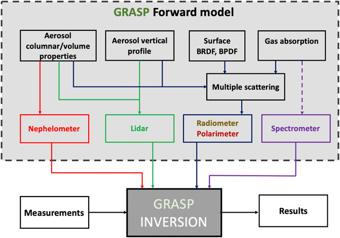
FIGURE 4. General organization of forward model and its connection with the numerical inversion in the GRASP algorithm.

Radiative transfer calculation accounting for multiple scattering effects in GRASP is implemented by on-line radiative transfer calculations using 1-D Successive Order of Scattering method. The scientific basis of this approach is documented in the paper by Lenoble et al. (2007). At the same time, some custom features are implemented in the radiative transfer module of GRASP as described by Dubovik et al. (2011). For example, the truncation procedure described by Waquet and Herman (2019) has been realized. The truncation procedure consists in removing the forward scattering peak observed in the phase function of large particles (few microns) or cloud droplets, due to diffraction. This approximation allows faster calculations for both total and polarized radiances and, as shown by Waquet and Herman (2019) maximal errors due to the used approximations do not exceed 0.001 for the degree of linear polarization for optical thickness smaller than 2.0, which is a sufficient accuracy for the most applications based on polarimetric measurements. In addition, several possibilities of using a number of trade-offs between the accuracy and the speed of the successive order of scattering method has been realized in GRASP (see Dubovik et al., 2011): including the possibilities of changing the number of terms M used in the expansion of the phase matrix into Legendre polynomials, the number of terms N used in Gaussian quadrature for zenithal integration, number of numerical layers in vertical atmosphere properties integrations, etc. Moreover, very recently the atmospheric correction approach was realized in the GRASP forward model. This approach decouples the radiative transfer effects of the atmosphere and surface in a rather original way and provides a simplified but still an accurate way of solving the radiative transfer equation (Litvinov et al., 2018). It provides sufficient accuracy for the atmospheric correction and high flexibility for further developments such as including adjacency effect, surface topology effect as well as the effect of cloud shadowing.

In addition, recently the radiative transfer module of GRASP has been extended by taking into account for the radiation coming from the thermal emission of the different atmospheric components and the surface (Herreras et al., 2020). In this realized implementation of the original 1-D Successive Order of Scattering numerical scheme by Lenoble et al. (2007) the source functions were extended to include Planck emission function. This modification allows for accounting the radiation coming from both scattering and emission origin in single and multiple scattering regimes. This new RT scheme accounting for emitted radiation has been validated against the reference radiative transfer code based on the discrete-ordinated method by Stamnes et al. (1988). The difference in the radiance, expressed in terms of brightness temperature, obtained from both codes under the same conditions is on average below 0.006 K. This difference is substantially below of the radiance accuracy of the most common instruments operating in thermal IR spectral range, like IASI (Blumstein et al., 2004) or CALIPSO IIR (Garnier et al., 2012) with an accuracy around 0.1 K. Thus, this realized RT development opened opportunity to apply GRASP approach for realizing atmospheric retrieval using both photometric and hyperspectral observations in visible and thermal IR spectral range.

The total surface reflectance matrix BRDM in GRASP code is modelled using Surface reflectance BRDF and BPDF. Specifically, as described in detail by Dubovik et al. (2011), 4 by 4 BRDM matrix is modelled using two terms M = M_diff + M_spec, where diffuse unpolarized term M_diff has only one non-zero element {M_diff}₁₁ modelled using semi-empirical BRDF function and specular reflection term is represented by Freshnel reflection function scaled by selected BPDF coefficient. Nevertheless, GRASP can operate also with more physically based models of the BPDF (Litvinov et al., 2012) when physical constraints can be imposed by the surface structure and composition. In general, both BRDF and BPDF can be calculated in GRASP using a variety of subroutines representing different models (Dubovik et al., 2011; Litvinov et al., 2011a; Litvinov et al., 2011b; Litvinov et al., 2012). The retrieval relies on water-land mask and uses either models of land or water surface reflectance. In the mixed observed pixels, both the properties of land and water surface reflectance models are retrieved and summed up in the 1-D radiative transfer using land/water fraction.

For the ocean surface the reflection is mainly governed by the wind speed at sea level as suggested by the Cox-Munk model (Cox and Munk, 1954). This model is employed in most applications including polarimetric observation (e.g., Deuzé et al., 1999; Deuzé et al., 2001; Herman et al., 2005; Xu et al., 2016; Xu et al., 2017, etc.) and also used in GRASP (see Dubovik et al., 2011 and some details in; Fougnie et al., 2019).

In a contrast, the reflection matrix from land surfaces may differ very strongly from location to location. Therefore, in the many algorithms interpreting satellite observation over land, the key aspect is correct determination of appropriate surface reflectance model and appropriate parameters. A number of BRDF models developed for surface reflectance description from remote sensing measurements are included into GRASP algorithm: Rahman-Pinty-Vestarte (RPV) model (Rahman et al., 1993), kernel-driven semi-empirical models (Ross-Li sparse, Ross-Li dense, Ross-Roujen models (Ross, 1981; Li and Strahler, 1992; Roujean et al., 1992; Wanner et al., 1995), physically-based models for bare soil and vegetated surfaces (Litvinov et al., 2012) as well as physically-based models for snow and ice (Kokhanovsky and Zege, 2004; Kokhanovsky and Breon, 2012). For polarimetric remote sensing these BRDF models are combined in GRASP algorithm with models for surface polarized reflectance (BPDF models). Most of the existent BPDF models are based on the Fresnel equations of light reflection from the surface. For example, Nadal and Bréon (1999) have proposed simple two-parameter non-linear function of the Fresnel reflection for characterization of atmospheric aerosol over land surfaces based on POLDER observations of land surface reflectance. Maignan et al. (2009) have introduced a new linear BPDF model with only one free parameter and demonstrated that this simple model allows a similar fit to the POLDER measurements as a more complex non-linear model by Nadal and Bréon (1999). For accurate description of polarimetric measurements like RSP (Research Scanning Polarimeter) airborne instrument, a three-parameter semi-empirical model was proposed by Litvinov et al. (2011a) and Litvinov et al. (2011b) (e.g., Rondeaux and Herman 1991, Nadal and Bréon, 1999; Maignan et al., 2004; Maignan et al., 2009; Waquet et al., 2009a; Waquet et al., 2009b; Litvinov et al., 2010; Litvinov et al., 2011a; Litvinov et al., 2011b). Analysis of number of airborne polarimetric measurements show minor spectral dependence of polarized reflectance in the visible and infrared spectral (e.g., Rondeaux and Herman 1991, Nadal and Bréon, 1999; Maignan et al., 2004; Maignan et al., 2009; Waquet et al., 2009a; Waquet et al., 2009b; Litvinov et al., 2010; Litvinov et al., 2011a; Litvinov et al., 2011b). At present time the parametrization of surface polarized reflectance with Fresnel-based BPDF models looks acceptable for existent polarimetric space-borne VIS and NIR observations.

BRDF and BPDF models included in GRASP are capable to reproduce reasonably the surface total and polarized reflectance (Maignan et al., 2004; Maignan et al., 2009; Litvinov et al., 2011a; Litvinov et al., 2011b) and have already been used for interpreting observations by MISR, MODIS, POLDER and other instruments (Justice et al., 1998; Martonchik et al., 1998; Govaerts et al., 2010; Wagner et al., 2010).

The actual choice of BRDF or BPDF models in practical application and retrieval approaches is always a subject of the discussion and, very often, depends on user preference. For global processing of different remote sensing measurements (PARASOL, MERIS, OLCI, S5p/TROPOMI and other) with GRASP algorithm the optimal balance between speed, accuracy linearity and number of parameters was provided by the combination of Ross-Li sparse BRDF model (Ross, 1981; Li and Strahler, 1992; Wanner et al., 1995) and one parametric Maignon-Breon model (Maignan et al., 2009). Nevertheless, other possible combinations of different BRDF and BPDF models are possible in GRASP algorithm and are always the subject of the studies on increasing retrieval performance.

Aerosol single scattering module is probably the most elaborated module of the GRASP algorithm that proposes a really large spectrum of different possibilities of approaching modeling optical properties of atmospheric aerosols. Indeed, in spite of the fact that GRASP is generally pursuing the retrieval of both aerosol and surface properties, it deeply relies on the heritage of aerosol retrieval advances (Dubovik et al., 1995; Dubovik et al., 2000; Dubovik and King, 2000; Dubovik et al., 2002; Dubovik, 2004; Dubovik et al., 2006) implemented for AERONET (see Holben et al., 1998) a worldwide network of currently over 600 radiometer sites that generate the data used to validate nearly all satellite observations of atmospheric aerosols. Currently, for all remote sensing applications aerosol can be modeled as a mixture of small polydisperse particles of various shapes and composition (Dubovik et al., 2006). Specifically, the optical properties of homogeneous layer of aerosol are defined by layer scattering and extinction optical thickness and by the elements of the scattering matrix $P_{\mathrm{ii΄}}\left(\lambda ;\Theta ;\mathrm{h}\right)$ that can be modeled with one or several aerosol components using microphysical properties of each component. Namely, as illustrated by Figure 5 each component aerosol component represents a mixture of particles with:

a) different size by defining the volume size distribution $\frac{d{V}_k\left(r\right)}{d\ln r};$

b) the different shapes using the mixture of randomly oriented spheroids with the distribution of axis or ratios $\frac{d{n}_k\left(\epsilon \right)}{d\ln \epsilon };$

c) spectral complex index of refraction $n_k\left(\lambda \right)$, $K_k\left(\lambda \right)$ and

d) vertical profile of aerosol component volume concentration $\frac{d{V}_k\left(h\right)}{d\ln h}$.

FIGURE 5

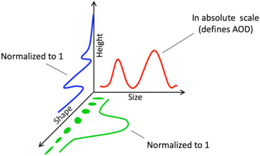
FIGURE 5. Illustration of modeling properties of each aerosol component in GRASP algorithm that is represented as a mixture of homogeneous particles that may have different sizes, spheroidal shapes, complex refractive indices and vertical profiles of concentrations.

Correspondingly, ${\tau }_{scat/ext}$ and $P_{\mathrm{ii΄}}\left(\lambda ;\Theta ;\mathrm{h}\right)$ of each homogeneus layer are modeled as the following:

${\tau }_{scat/ext}={\displaystyle \sum _{k=1}^K\left(\underset{\ln h_{\min }}{\overset{\ln h_{\max }}{\int }}\underset{\ln {\epsilon }_{\min }}{\overset{\ln {\epsilon }_{\min }}{\int }}\underset{\ln r_{\min }}{\overset{\ln r_{\max }}{\int }}\frac{C_{scat/ext}\left(n_k\left(\lambda \right);k_k\left(\lambda \right);h;\epsilon ;r\right)}{V\left(r\right)}\frac{d{V}_k\left(h\right)}{d\ln h}\frac{d{n}_k\left(\epsilon \right)}{d\ln \epsilon }\frac{d{V}_k\left(r\right)}{d\ln r}d\ln hd\ln \epsilon d\ln r\right)}$(3.1)

and

${\tau }_{scat}{P}_{\mathrm{ii΄}}\left(\lambda ;\Theta ;\mathit{h}\right)={\displaystyle \sum _{k=1}^K\left(\underset{\ln h_{\min }}{\overset{\ln h_{\max }}{\int }}\underset{\ln {\epsilon }_{\min }}{\overset{\ln {\epsilon }_{\mathrm{mix}}}{\int }}\underset{\ln r_{\min }}{\overset{\ln r_{\max }}{\int }}\frac{C_{\mathrm{ii΄}}\left(\Theta ;n_k\left(\lambda \right);k_k\left(\lambda \right);h;\epsilon ;r\right)}{V\left(r\right)}\frac{d{V}_k\left(h\right)}{d\ln h}\frac{d{n}_k\left(\epsilon \right)}{d\ln \epsilon }\frac{d{V}_k\left(r\right)}{d\ln r}d\ln hd\ln \epsilon d\ln r\right)}$(3.2)

Here, as illustrated by Figure 5, each component is described by the size distribution $\frac{d{V}_k\left(r\right)}{d\ln r}$, shape distribution $\frac{d{n}_k\left(\epsilon \right)}{d\ln \epsilon }$, spectral complex index of refraction $n_k\left(\lambda \right)$, $K_k\left(\lambda \right)$ and vertical profile $\frac{d{V}_k\left(h\right)}{d\ln h}$, where λ denotes wavelength, Θ – scattering angle, h - height of the layer, ε - axis ratios of spheroid, and r denotes radius of volume equivalent sphere and $C\left(n_k\left(\lambda \right);K_k\left(\lambda \right);h;\epsilon ;r\right)$ is a cross-section of extinction, total or angular scattering of aerosol particle.

All these characteristics of aerosol component can be modeled using approaches of different complexity.

Aerosol size distribution $\frac{d{V}_k\left(r\right)}{d\ln r}$ - can be modeled:

• using a representation of the size distribution as a superposition of triangular N_i bins by retrieving concentration of each bin $\frac{d{V}_k\left(r_i\right)}{d\ln r}$ for each radii r_i. This approach is used in AERONET retrieval by Dubovik and King (2000);

• using a representation of the size distribution as a superposition of log-normal N_i bins by retrieving concentration of each log-normal bin $\frac{d{V}_k\left(r_i\right)}{d\ln r}$. This approach is described in Dubovik et al. (2011). Each log-normal bin may have different position and width. This approach is more appropriate when only very limited number of bins is used;

• using a bi-modal log-normal approximation of the size distribution. In this case the parameters of bi-modal log-normal function are retrieved (see Dubovik et al., 2011). This approximation is extensively used by Torres et al. (2017) for inverting measured AOD.

• using the size distribution with the fixed shape of size distribution (using any of above modeling approaches). In this case only total volume of the aerosol component is retrieved.

Aerosol shape distribution $\frac{d{n}_k\left(\epsilon \right)}{d\ln \epsilon }$ - is simulated assuming aerosol as mixture of randomly oriented spheroids using of pre-computed spheroid kernels software described by Dubovik et al. (2006). The following approaches for modeling shape distribution are realized using detailed shape distribution defined as $\frac{d{n}_k\left({\epsilon }_i\right)}{d\ln \epsilon }=q_{k,i}$, where.

• $q_{k,i}$ is a fraction of k-th aerosol component particles with axis ${\epsilon }_i$.

• $q_{k,i}$ is a fraction of particles of k-th aerosol component with j-th predetermined shape distribution. The definition of two or more fractions can be defined in nearly arbitrary way within the pre-calculated spheroid kernels by Dubovik et al. (2006).

For example, for AERONET (Dubovik et al., 2006) and POLDER (Dubovik et al., 2011) retrievals only two fractions used $q_{k,\epsilon =1}$ - fraction of spherical particles and $q_{k,\epsilon \ne 1}=1-q_{k,\epsilon =1}$ - fraction of non-spherical particles (with fixed shape distribution). In that case only one parameter $q_{k,\epsilon =1}$ is retrieved. The non-spherical component of aerosol in that case is simulated using axis ratio obtained by Dubovik et al. (2006) from fitting the desert dust phase matrix measurements by ensemble of spheroids [see detailed desctiption in the paper by Dubovik et al. (2006) and Dubovik et al. (2011)].

Aerosol vertical distribution $\frac{d{V}_k\left(h\right)}{d\ln h}$ can be defined in the following ways:

• the profile is defined as an exponential profile $\frac{d{V}_k\left(h\right)}{dh}\sim {\mathit{e}}^{\mathit{-h/}\alpha }$. The profile is normalized to unity and scale height α is retrieved parameter.

• the profile is defined as Gaussian profile $\frac{d{V}_k\left(h\right)}{dh}\sim {\mathit{e}}^{\mathrm{-}\frac{\mathrm{1}}{\mathrm{2}}\frac{{\left(\mathrm{h-}{\mathrm{h}}_{\mathrm{0}}\right)}^2}{\mathrm{\hspace{0.17em}}{\sigma }_{\mathit{h}}^{\mathrm{2}}}}$. The profile is normalized to unity, the mean height h₀ and standard deviation ${\sigma }_h$ can be retrieved.

• the profile is defined as a superposition of N_i triangular bins by retrieving concentration of each bin $\frac{d{V}_k\left(h_i\right)}{d\ln h}=C_{h,i}$ for each height h_i. This is similar approach as used above for modeling size distribution, more details and illustration of the approach are provided by Lopatin et al. (2013) and Lopatin et al. (2021).

It should be noted that as illustrated in Figure 5 the aerosol shape $\frac{d{n}_k\left({\epsilon }_i\right)}{d\ln \epsilon }=q_{\epsilon ,i}$ and vertical $\frac{d{V}_k\left(h_i\right)}{d\ln h}=C_{h,i}$ distributions are always retrieved in form of fractions. For example, for vertical profile $\frac{d{V}_k\left(h_i\right)}{d\ln h}=C_{h,i}$ it is always assumed:

${\displaystyle \sum _{i=1,\dots ,N_h}{C}_{h,i}=1}$(3.3)

Using the above constraint, the following N_h-1 values are retrieved in GRASP:

${\mathit{a}}_{\mathrm{i}}=\frac{C_{h,i+1}}{C_{h,1}}\left(i=1,\dots ,N_h-1\right)$(3.4)

Correspondingly,

$C_{h,1}=\frac{1}{\left(1+{\displaystyle \sum _{i=1,\dots ,N_h-1}{\mathit{a}}_i}\right)}\mathrm{a}\mathrm{n}\mathrm{d}{C}_{h,i+1}=C_{h,1}{\mathit{a}}_{\mathrm{i}}\left(i=1,\dots ,N_h-1\right)$(3.5)

The above is written for the case when the profile grid points are constant, i.e.

${\Delta }_i=\ln h_{i+1}-\ln h_i=const$(3.6)

If ${\Delta }_i$ is not constant then Eq. 3.5 should be rewritten as

${\mathit{C}}_{\mathit{h,1}}=\frac{2}{1+{\displaystyle \sum _{i=1,\dots ,N_h-1}{\mathit{a}}_i}\left({\Delta }_i+{\Delta }_{i+1}\right)}$(3.7)

Size distribution can also be retrieved using fractions of particle different sizes:

${\mathit{a}}_{\mathrm{i}}=\frac{\frac{d{V}_k\left(r_{i+1}\right)}{d\ln r}}{\frac{d{V}_k\left(r_1\right)}{d\ln r}}\left(i=1,\dots ,Nr-1\right)$(3.8)

However, in that case, together with N_r -1 a_i parameters the total concentration C_r is also retrieved:

$C_r={\displaystyle \sum _{i=1,\dots N_r}\frac{d{V}_k\left(r_i\right)}{d\ln r}}$(3.9)

Retrieving C_r and N_r-1 a_i parameters allows for separating the parameter defining the total amount of particles with the set of parameters a_i defining shape of size distribution.

Complex index of refraction: $n\left(\lambda \right)$-real and $k\left(\lambda \right)$ -imaginary parts of the refractive index can be defined using several different strategies:

• the spectral values $n\left({\lambda }_i\right)$ and $k\left({\lambda }_i\right)$ are retrieved for each wavelength in similar way as it is realized for AERONET (Dubovik and King, 2000) and POLDER (Dubovik et al., 2011) retrievals;

• the spectral values $n\left({\lambda }_i\right)$ and $k\left({\lambda }_i\right)$ are modeled as a homogeneous mixture of different aerosol components mixed internally. At present there are two possibilities in GRASP [see details in Li et al. (2019)]:

i)- several aerosol components with known spectral dependencies $n\left(\lambda \right)$ and $k\left(\lambda \right)$ are mixed internally using Maxwell-Garnett effective medium approximation: the particles are composed of black carbon, brown carbon, absorbing insoluble, non-absorbing insoluble embedded in a soluble host.

ii)- several aerosol components with known spectral dependencies $n\left(\lambda \right)$ and $k\left(\lambda \right)$ are mixed internally proportionally to the volume fraction of each component including black carbon, brown carbon, iron oxide, non-absorbing mineral dust, etc.

• the spectral values $n\left({\lambda }_i\right)$ and $k\left({\lambda }_i\right)$ can be assumed and fixed for each aerosol component.

The aerosol modeling options described above are suitable for retrievals when such aerosol parameters as size, shape, spectral refractive index and vertical distribution can be explicitly retrieved. However, in the situations with limited information content retrieval of those detailed characteristics could be challenging or impossible. In such a situation, the aerosol single scattering properties can be modelled as an external mixture of several aerosol components and the columnar properties of each component:

${\tau }_{scat/ext}={\displaystyle \sum _{k=1}^K{C}_v^k{\rho }_{scat/ext}^k\left(\lambda \right)}$(3.10)

and

${\tau }_{scat}{P}_{\mathrm{ii\text{'}}}\left(\lambda ;\Theta ;\mathrm{h}\right)={\displaystyle \sum _{k=1}^K{C}_v^k{\rho }_{scat/ext}^k\left(\lambda \right)}{P}_{\mathrm{ii\text{'}}}^{\mathrm{k}}\left(\lambda ;\Theta ;\mathrm{h}\right)$(3.11)

where ${\rho }_{scat/ext}^k\left(\lambda \right)$ and $P_{\mathrm{ii\text{'}}}^{\mathrm{k}}\left(\lambda ;\Theta ;\mathrm{h}\right)$ denote the scattering/extinction per unit of volume and phase matrix of each aerosol component that are pre-calculated using complex refractive index, size and shape distributions assumed for each aerosol component. Correspondingly, only K concentrations drive the modeling of columnar properties of aerosol. The number of the retrieved parameters is significantly reduced in this approach, which is helpful for the observations with limited sensitivity to the size, shape and refractive index of the aerosol particles. For example, as will be discussed below this approach was successfully employed in processing MERIS and POLDER satellite data by GRASP. Also, as discussed by Lopatin et al. (2021) this approach is rather suitable for processing vertically resolved observations by lidar or airborne radiosonde data. In applications to MERIS and POLDER satellite data, the vertical aerosol distribution was assumed the same for all the components and modeled as Gaussian or exponential function, while in processing of vertically resolved observations a detailed separate vertical distribution can be retrieved for each aerosol component. In general, the aerosol components are associated with optically distinct types of aerosol based on particle sizes, scattering and absorption capabilities, etc. For example, in GRASP applications to MERIS, POLDER, lidar and radiosonde data, the aerosol components were defined based on AERONET climatology by Dubovik et al. (2002) and Smirnov et al. (2002), the exact definitions are discussed by Lopatin et al. (2021). At the same time, these components can be easily redefined and modified in frame of GRASP software.

Thus, aerosol in GRASP retrieval can be represented as rather sophisticated mixture of one or several aerosol components that can differ by particle size distribution, shape distribution, vertical profile and complex index of refraction. All these characteristics can be either assumed and fixed or retrieved. The complexity of modeling each of these characteristics depends on the information content of observations used in each specific GRASP application.

Gaseous absorption can also be fully accounted in GRASP forward modeling of atmospheric radiances. The possibility of rigorous accounting for atmospheric gases absorption was recently incorporated with the help of the team from Free University of Berlin with an objective to explore the synergy between photometric and spectrometric observations and combined retrieval of properties of both atmospheric aerosol and gases. The rationale of such an approach is in improving the accuracy of atmosphere components characterization. Indeed, the gases and aerosol affect radiation very differently, and, therefore, very different measurements are used for their retrieval. For example, Figure 6 illustrates a typical spectral dependence of extinction by atmospheric gases, and fine (radius < ∼ 0.5 micron) and coarse (radius > ∼ 0.5 micron) aerosol particles using complex refractive index of quartz. It is clear from this illustration that absorption of atmospheric gases has much finer spectral features than aerosol, especially in visible spectral range.

FIGURE 6

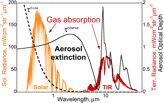
FIGURE 6. The displayed extinction for fine (radius < ∼ 0.5 micron) and coarse (radius > ∼ 0.5 micron) aerosol particles was calculated using complex refractive index of quartz.

Therefore, in practice most commonly the retrievals of aerosol and gases are separated. In general, radiometers are used to make measurements in only a few selected spectral “window” channels with minimal gaseous absorption with the purpose to characterize aerosol properties. In a contrast, the gaseous retrievals tend to rely on the hyper-spectral features of gaseous absorption observed by spectrometers, with aerosol contribution subtracted as smooth “background”. In these regards, the current version of GRASP allows joint retrieval of both aerosol and gases from joint spectrometric and photometric observations.

Equation 3.12 illustrates the modeling of the transmitted radiances on the properties of atmospheric aerosol, gases and molecular scattering for cloud-free atmosphere.

$\begin{array}{l}\mathrm{I}\left(\lambda \mathit{,h}\right)\mathrm{\sim }{\displaystyle \underset{{\lambda }_{\min }}{\overset{{\lambda }_{\max }}{\int }}\mathbf{\Omega }\left(\lambda \right)I_0\left(\lambda \right)\left(\mathit{e}\mathbf{-}\mathit{m}\left(\underset{\mathrm{0}}{\overset{\mathit{h}}{\int }}\left({\displaystyle \sum _{\mathit{i=1}}^{{\mathit{N}}_{\mathit{gas}}}{N}_i\left(\mathit{h}\right)C_{i,abs}^{gas}\left(\lambda ,T\left(\mathit{h}\right),P\left(\mathit{h}\right)\right)+C_{\mathit{ext}}^{\mathit{aer}}\left(\lambda ,\mathit{h}\right)+C_{\mathit{ext}}^{\mathit{mol}}\left(\lambda ,\mathit{h}\right)}\right)\mathit{dh}\right)+\mathit{mult}\mathit{scat}\right)d\lambda =}\\ ={\displaystyle \underset{{\lambda }_{\min }}{\overset{{\lambda }_{\max }}{\int }}\left(\mathbf{\Omega }\left(\lambda \right)I_0\left(\lambda \right)\left({\mathit{e}}^{\mathbf{-}\mathit{m}\left({\tau }_{abs}^{gas}\left(\lambda \right)+{\tau }_{ext}^{aer}\left(\lambda \right)+{\tau }_{ext}^{mol}\left(\lambda \right)\right)}+\mathit{mult}\mathit{scat}\right)\right)d\lambda }\end{array}$(3.12)

where ${\mathit{N}}_{\mathrm{i}}\left(\mathit{h}\right)$ is profile of i-th gas concentration, the cross-section of gaseous absorption $C_{i,abs}^{gas}\left(\lambda ,T\left(h\right),P\left(h\right)\right)$ depends on temperature (T) and pressure (P) and $\mathbf{\Omega }\left(\lambda \right)$ denotes spectral filter function. At the moment, GRASP forward model can account in monochromatic calculations for any gas in any spectral range for a maximum of ten different gaseous species simultaneously using a line-by-line approach. The calculations of the radiative flux calculations realized in GRASP [as described by Derimian et al. (2016)] also account for such details as dependence of water vapor absorption cross section on its concentration due to continuum (e.g., see Kato et al., 1999). The vertical profiles of pressure and temperature are to be provided as an additional and necessary input for line-by-line calculations. In order to speed up the calculations, the look-up-tables with the absorption spectral information for each considered gas species are used. These look-up-tables of absorption values are usually pre-calculated for a wide range of pressures, temperatures and wavelengths and stored into look-up-tables that are later called in the retrieval. As a result, only a renormalization to the required concentration and a simple interpolation to the defined pressure and temperature profile are needed to obtain the gas absorption profile. In order to obtain these pre-calculated values the CGASA line-by-line model (developed by the Institute for Space Sciences, Free University Berlin) is used. Notwithstanding, the look-up-table format is readable, easy to understand and it is open to the users to include their own look-up-tables which fulfill their requirements.

However, direct spectral integration of line-by-line fine structure requires consideration of a very large number of channels with full accounting for multiple scattering for each channel. Such direct implementation of the spectral integration has high accuracy but is highly time consuming. Therefore, an alternative methodology called a “k-distribution approach” (see Doppler et al., 2014) is also been integrated into GRASP forward model to speed up the integration time. The accuracy of this methodology is somewhat reduced compared to line-by-line procedure but sufficient for most remote sensing applications. The k-distribution methodology relies on the same basic assumption of smooth aerosol spectral behavior and reduces the number of multiple scattering runs for the spectral integration to about 10 or even less instead of thousand. Specifically, the approach sorts the gaseous absorption coefficients “k” within the spectral function to a limited set of bins (∼10) by the magnitude of the coefficients and then implements only a single multiple scattering run for each “k” bin.

It should be noted that the calculation of the k-distribution kernels themselves are generated externally and need to be prepared as input prior using k-distribution modeling in GRASP. The dependence of GRASP on external sources to use this technique can be considered as a drawback. At the same time, the fully standardized format of this input information in GRASP allows the utilization of a vast variety of different principles (Uncorrelated, TOA-correlated, Layer-Correlated, etc.) and algorithms that can be used to calculate k-distribution parameters. The user can select the specific methodology to match the specific requirements in each situation and is not forced to use one specific approach.

Thus, depending on available measurements and information both the profiles of gaseous concentrations as well as temperature and pressure can be determined.

4 Multi-Term LSM: Retrieval Practice Using GRASP

GRASP algorithm was designed as generalized approach that could be used in diverse remote sensing applications (see introduction by Dubovik et al. (2014)]. Indeed, the Multi-term LSM approach employed for numerical inversion and forward model allowing simulations of transmitted and reflected radiation in the atmosphere allows an efficient exploitation of the GRASP algorithm for diverse applications for atmospheric remote sensing including retrieval of detailed properties of aerosol particles from laboratory and in situ observations, as well as from ground-based, airborne and satellite passive and active remote sensing observations. GRASP also retrieves detailed properties of underlying surface reflectance from down-looking satellite and airborne observations. In addition, due to very general principles realized for inversion and forward model calculations, GRASP application scope is expected to be significantly expanded, so that it can be used for applying both radiometric and hyper spectral observations in a wide spectral range from ultra violet (UV) to thermal infrared (TIR) and retrieving not only aerosol and surface properties but also properties of atmospheric gases and clouds. Some applications for retrieving properties of hydrosols can also be envisioned.

4.1 Laboratory and In Situ Observations of Aerosol Single Scattering

Laboratory and in situ instrumentation generally can provide more detailed and elaborated measurements of radiances transmitted and diffused by a sample of air volume or surface area compared to the remote sensing using ground-based, airborne or satellite measurements. For example, using laboratory and in situ instruments most of the single scattering characteristics, ${\tau }_{scat/ext}$ and the elements of scattering matrix $P_{\mathrm{ii΄}}\left(\lambda ;\Theta ;\mathit{h}\right)$ can be directly measured. Using the approach described by Eq 3.1, 3.2 these characteristics can be simulated by GRASP based on known microphysical aerosol properties (particle size distribution, shape parameter, etc.). Inversely, if measurements of ${\tau }_{scat/ext}$ and/or $P_{\mathrm{ii΄}}\left(\lambda ;\Theta ;\mathit{h}\right)$ are available, the microphysical properties of the aerosol can be retrieved by GRASP.

The retrieval of aerosol microphysical properties from the measurements of the phase matrix $P_{\mathrm{ii΄}}\left(\lambda ;\Theta ;\mathit{h}\right)$ elements at several wavelengths (together with or without ${\tau }_{scat/ext}$) is the base for more challenging remote sensing satellite and ground-based observations. Indeed, such angular remote sensing observations from satellite and ground-based instruments are less detailed and affected by complex multiple scattering effects.

The angular measurements of $P_{\mathrm{ii΄}}\left(\lambda ;\Theta ;\mathit{h}\right)$ in a wide range of scattering angels (∼from 0° to 180°) at several wavelengths contain practically maximal information about aerosol microphysical properties, especially if these angular measurements are complimented with spectral measurements of total scattering or extinction ${\sigma }_{scat/ext}$ of the aerosol sample. Therefore, the retrieval of practically all aerosol characteristics can be expected from such detailed measurements. For example, in studies by Dubovik et al. (2006) such properties as detailed size and shape (axis or aspects ratios) distributions were retrieved together with spectral complex index of refraction from laboratory measurements of aerosol samples phase matrices. In the framework of GRASP software, the inversion of full scattering matrix (6 elements) at any wavelengths and for any angular range selection together with the spectral measurements of ${\sigma }_{scat/ext}\left(\lambda ,h\right)$ is realized. In addition, the measurements of any simple functions of $P_{\mathrm{ii΄}}\left(\lambda ;\Theta ;\mathit{h}\right)$ and ${\sigma }_{scat/ext}\left(\lambda ,h\right)$ can be easily added if required. For example, the measurements of total absorption ${\sigma }_{abs}\left(\lambda ,h\right)$, backscattering $\beta \left(\lambda ,180\mathrm{°},\mathit{h}\right)$ or total scattering ${\sigma }_{scat}\left(\lambda ,{\Theta }_{\min },{\Theta }_{\max },h\right)$ in the selected range of scattering angles: ${\Theta }_{\min }\le \Theta \le {\Theta }_{\max }$ can be included in the set of inverted single scattering properties with GRASP. From the practical viewpoint the inversion of the phase function $P_{\mathrm{11}}\left(\lambda ;\Theta ;\mathit{h}\right)$ (or angular scattering ${\sigma }_{scat}\left(\lambda ,h\right)P_{\mathrm{11}}\left(\lambda ;\Theta ;\mathit{h}\right)$) and linear polarization $P_{\mathrm{12}}\left(\lambda ;\Theta ;\mathit{h}\right)$ at several wavelengths (together with or without ${\tau }_{scat/ext}$) is one of the most popular applications. Indeed, most of passive remote sensing techniques using angular information based on the measurement of atmospheric radiation characterized by $I\left(\lambda ;\Theta ;\mathit{h}\right)$ element of Stocks vector (e.g., see Mishchenko et al., 2006) and linear polarization characterized by $Q\left(\lambda ;\Theta ;\mathit{h}\right)$ and $U\left(\lambda ;\Theta ;\mathit{h}\right)$ elements of Stocks vector. In single scattering approximation, $I\left(\lambda ;\Theta ;\mathit{h}\right)$, $Q\left(\lambda ;\Theta ;\mathit{h}\right)$ and $U\left(\lambda ;\Theta ;\mathit{h}\right)$ measured at the top or bottom of the atmosphere depends only on $P_{\mathrm{11}}\left(\lambda ;\Theta ;\mathit{h}\right)$ and $P_{\mathrm{12}}\left(\lambda ;\Theta ;\mathit{h}\right)$. Some other elements of phase matrix contribute to $I\left(\lambda ;\Theta ;\mathit{h}\right)$, $Q\left(\lambda ;\Theta ;\mathit{h}\right)$ and $U\left(\lambda ;\Theta ;\mathit{h}\right)$ only via rather complex multiple scattering interactions of solar radiation with the atmosphere. Therefore, the single scattering contributions of $P_{\mathrm{11}}\left(\lambda ;\Theta ;\mathit{h}\right)$ and $P_{\mathrm{12}}\left(\lambda ;\Theta ;\mathit{h}\right)$ often dominate passive radiometric and polarimetric remote sensing measurements. Correspondingly, the retrieval of aerosol microphysical properties from the measured phase function $P_{\mathrm{11}}\left(\lambda ;\Theta ;\mathit{h}\right)$ together with (or without) linear polarization $P_{\mathrm{12}}\left(\lambda ;\Theta ;\mathit{h}\right)$ at several wavelengths can be considered as a base for a more challenging remote sensing satellite and ground-based observations.

Therefore, the development of aerosol property retrievals from angular measurements of the phase function and linear polarization helps to obtain understanding of a retrieval’s potential and to design relevant remote sensing approaches. In these regards, in the framework of GRASP the potential for a wide diversity of retrievals can be evaluated on the basis of single scattering sensitivity tests. For example, there are a number of cases where the phase function and linear polarization was measured directly and used for the retrieval of detailed aerosol properties with the help of the GRASP approach, including studies by (Dolgos and Martins, 2014; Espinosa et al., 2017; Espinosa et al., 2019 W. R.; Puthukkudy et al., 2017; Schuster et al., 2019, etc.). A demonstration of one such retrieval study using measurements of polystyrene (PSL) spheres from Espinosa et al. (2017) is shown in Figure 7.

FIGURE 7

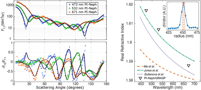
FIGURE 7. The results of a study using GRASP to characterize the size and refractive index of monodisperse polystyrene spheres from multiwavelength polar nephelometer measurements. (A): scattering matrix element measurements (circles) at 473, 532 and 671 nm obtained from a PSL sample along with the corresponding GRASP fits (solid lines). (B): retrieved real part of the refractive index, alongside three prior measurements of PSL refractive index (Ma et al., 2003; Sultanova et al., 2003; Jones et al., 2013). The embedded subplot in the upper-right corner shows the GRASP retrieved size distribution (blue) alongside the manufacturer’s specified central radius (red dashes) and ±0.5σ distribution width (red dots).

In addition, such remote sensing observations such as aerosol optical depth or lidar backscattering measured from the ground are sensitive mainly to single scattering aerosol properties and generally modeled using the single scattering approximation. The application of GRASP for these observations will be considered below.

4.2 Ground-Based Passive Observations

GRASP approach is developed based on the heritage of AERONET retrieval developments by Dubovik and King (2000), Dubovik et al. (2000) and Dubovik et al. (2006). Therefore, GRASP can be used for inversion of AERONET-like radiometric ground-based observation data in a similar way as it is done in AERONET operational aerosol retrieval. Therefore, applying GRASP to such data should provide essentially similar retrieval results. At the same time, even though GRASP has adapted the main conceptual elements from the AERONET retrieval, the actual algorithm is different, therefore some minor differences can be observed even in the identical application.

The potential of applying GRASP to radiometric ground-based observations lies in the possibilities of trying and evaluating new retrieval concepts. Indeed, as described above in Theory of Multi-Term LSM Inversion, GRASP allows one to use a variety of the retrieval setups. For example, in difference with AERONET operational retrieval, it is possible to attempt deriving more detailed shape distribution, to employ multi-component aerosol mixture with different refractive indices for each component, to approximate size distribution by log-normal functions, etc. The examples of such diverse AERONET inversions can be found in a number of published studies. Li et al. (2019) demonstrated the retrieval of aerosol properties from AERONET observations assuming aerosol as a mixture of different aerosol components. As it was demonstrated this approach allows adequate modeling of aerosol AERONET observation and the retrieved results provide some inside on aerosol composition. Torres et al. (2014) made extensive analysis of aerosol retrieval sensitivity to geometrical configuration of ground-based sun/sky-radiometer observations. This study was conducted using GRASP algorithm, and employed different assumption of aerosol vertical variability in the series of synthetic tests. In more recent studies the GRASP based methodology was established for retrieving aerosol properties from only direct Sun AERONET observation of optical thickness. Torres et al. (2017) describe the “GRASP-AOD” approach in details and Torres and Fuertes (2020) demonstrate extensive application of the method to AERONET AOD observations. GRASP-AOD uses the assumptions of bi-modal lognormal size distribution and provides AOD of fine and coarse aerosol modes (AODF and AODC). The results of comparisons by Torres and Fuertes (2020) have shown that GRASP-AOD provides AODF and AODC comparably good and sometimes even better accuracy than the established retrieval approaches by O’Neill et al. (2003) and Perez-Ramirez et al. (2015). In addition, GRASP-AOD provides information about aerosol size distribution including concentrations, standard deviations, median and effective radii of total, fine and coarse modes of aerosol size distributions. These retrieved aerosol properties agree well with the results of full AERONET retrieval performed for the same AOD observations.

GRASP also can be used for inverting diverse non-AERONET observations from ground or AERONET observations that generally included in AERONET processing. For example, Torres and Fuertes (2020) demonstrated aerosol retrieval using direct Sun AOD observation combined with the sky-radiances measured in solar aureole. Such retrieval showed to provide superior about aerosol size distribution compare to GRASP-AOD only retrieval and can be applied to the AERONET data acquired in partially cloudy environment. Roman et al. (2017, 2021) applied GRASP for aerosol retrieval from the measurements by lunar aureole with a sky camera. Torres et al. (2017) and Popovici et al. (2018) have applied GRASP-AOD approach for interpretation of AOD observations by lunar-photometer. The upper panel of Figure 8 illustrates the size distribution by GRASP-AOD from AOD observations by lunar-photometers. The lower panel of Figure 9 illustrates the improvements in the aerosol retrieval by inverting radiances measured in solar aureole together with AOD data compare to inversion of AOD data only (Torres and Fuertes, 2020).

FIGURE 8

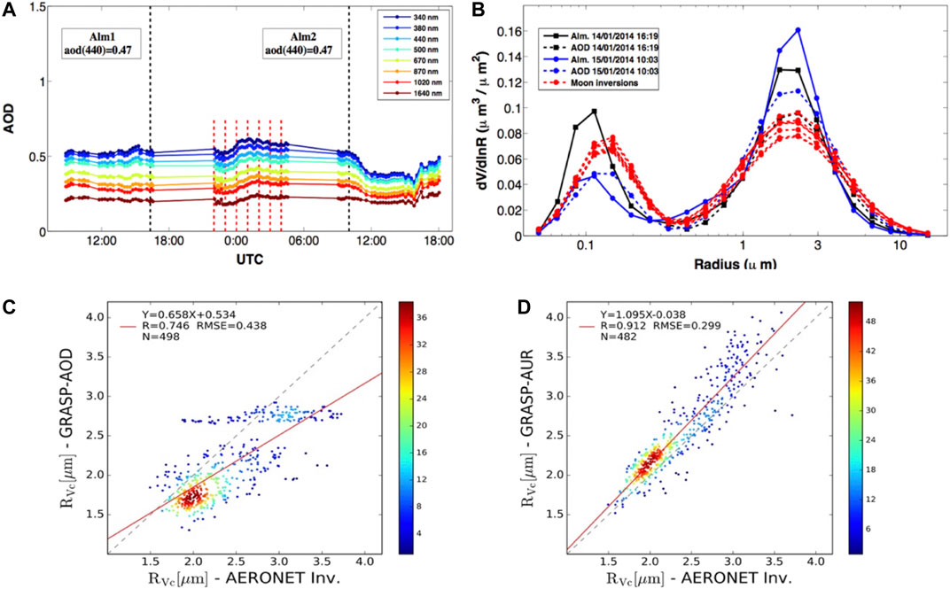
FIGURE 8. The application of GRASP-AOD for inverting direct Sun and Moon observations. (A): illustration of daily AERONET and nocturne Moon photometer AOD observations in Dakar site during April 14, 15, 2014. The vertical dashed lines correspond to almucantar observations; (B): the compassion of size distributions derived by GRASP-AOD approach from AOD obtained from direct Sun and Moon observation with regular AERONET inversions (Torres et al., 2014). The comparison of retrieval of aerosol properties by GRASP from AOD only data (GRASP-AOD) and from AOD data together with the measurement of radiances in the aureole in applying the retrieval to 2 years of the ARONET data over Granada site. (C): the correlation of retrieved R_Vcc from AOD data (GRASP-AOD) with full AERONET retrieval. (D): the correlation of retrieved mean volume radius of aerosol coarse mode (R_Vcc) from AOD and radiances in the aureole data (GRASP-AUR) with full AERONET retrieval (Torres and Fuertes, 2020).

FIGURE 9

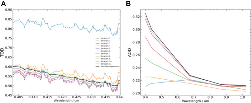
FIGURE 9. The illustration of the inversion dynamics evolution through at the different iterations. (A): fitting of direct Sun hyperspectral observations of Pandora. (B): evolution of the retrieved AOD values.

It is important to underline that GRASP allow rather straightforward use of ground-based radiometric observations in the retrievals using synergy with other ground-based, satellite or air-borne observations. For example, the combined processing of ground-based radiometric and lidar observations as will be discussed in next sections.

Finally, as described in Theory of Multi-Term LSM Inversion, several new modules were integrated into GRASP forward model for making it possible to simulate both photometric and hyperspectral observations in visible and thermal IR part of the spectrum. Therefore, at present GRASP is ready for a processing not only photometric but also spectrometric ground-based observations in wide spectral range. Specifically, very recently first tests have been done with application of GRASP to combined inversion AERONET type radiometric observation together with CLIMAT thermal TIR radiometer (Legrand et al., 2000; (Brogniez et al., 2003) or PANDORA spectrometer (Herman et al., 2015). These developments are yet at early stages, nonetheless the first test indicate high potential for these new applications. For example, AERONET/CLIMAT retrieval will allow the retrieval of a consistent aerosol optical characteristic in wide visible-TR spectral range and synergy inversion of joint AERONET and PANDORA observations is promising for improved simultaneous retrieval of aerosol and such atmospheric gases as NO2 and Ozone (Herreras-Giralda et al. in preparation). These applications were overall realized and tested with synthetic data, where NO2 are retrieved simultaneously with aerosol. Figure 9 illustrates the synthetic retrieval applied to a combined data set including almost 150 Pandora channels ranging from 400 to 440 nm, and the four standard AERONET channels (440, 675, 870 and 1,020 nm). In this application GRASP algorithm successfully operates with the hyperspectral features of gas absorption and the smooth aerosol optical characteristics. The real data inversion results of this combined retrieval of aerosol and NO2 have been done using DIVA (see Synergetic Retrievals and Other Diverse GRASP Applications) platform and initial validation has been done against independent algorithms as AERONET, for aerosol, and PGN (Pandonia Global Network) (Herman et al., 2009; Tzortziou et al., 2012) for gas related products.

Thus, GRASP is being expanded for retrieval of also atmospheric gases in addition to aerosol and surface. Moreover, some very recent developments are initiated to include cloud retrieval in GRASP framework. Theretofore, to reflect this development, it is appropriate to rename GRASP as Generalized Retrieval of Atmosphere and Surface Properties instead of Generalized Retrieval of Aerosol and Surface Properties.

4.3 Ground-Based Active Observation and Synergy With Passive Observations

Initially the possibilities of processing active lidar observation were integrated into GRASP by Lopatin et al. (2013) as part synergetic GARRLiC (Generalised Aerosol Retrieval form Radiometer and Lidar Combination) retrieval that inverts simultaneously the photometric and lidar observations. Since then GARRLiC/GRASP has been employed and discussed in numerous studies (Benavent-Oltra et al., 2017; Benavent-Oltra et al., 2019; Benavent-Oltra et al., 2021; Hu et al., 2019; Tsekeri et al., 2013; Tsekeri et al., 2017; Roman et al., 2018; Titos et al., 2019; Molero et al., 2020; Parajuli et al., 2020; Konsta et al., 2021 etc.). Moreover, it is currently being employed for operational processing of such combined data in the frame of the European ACTRIS infrastructure (https://www.actris.eu/). The standard GaRRLiC approach by Lopatin et al. (2013) inverts spectral lidar data together with sun/sky scanning AERONET like radiometer, and the detailed columnar size distributions, and spectral complex index of refraction can be retrieved for two fine and coarse aerosol components together with two vertical profiles of their concentration can be derived as illustrated by Figure 10.

FIGURE 10

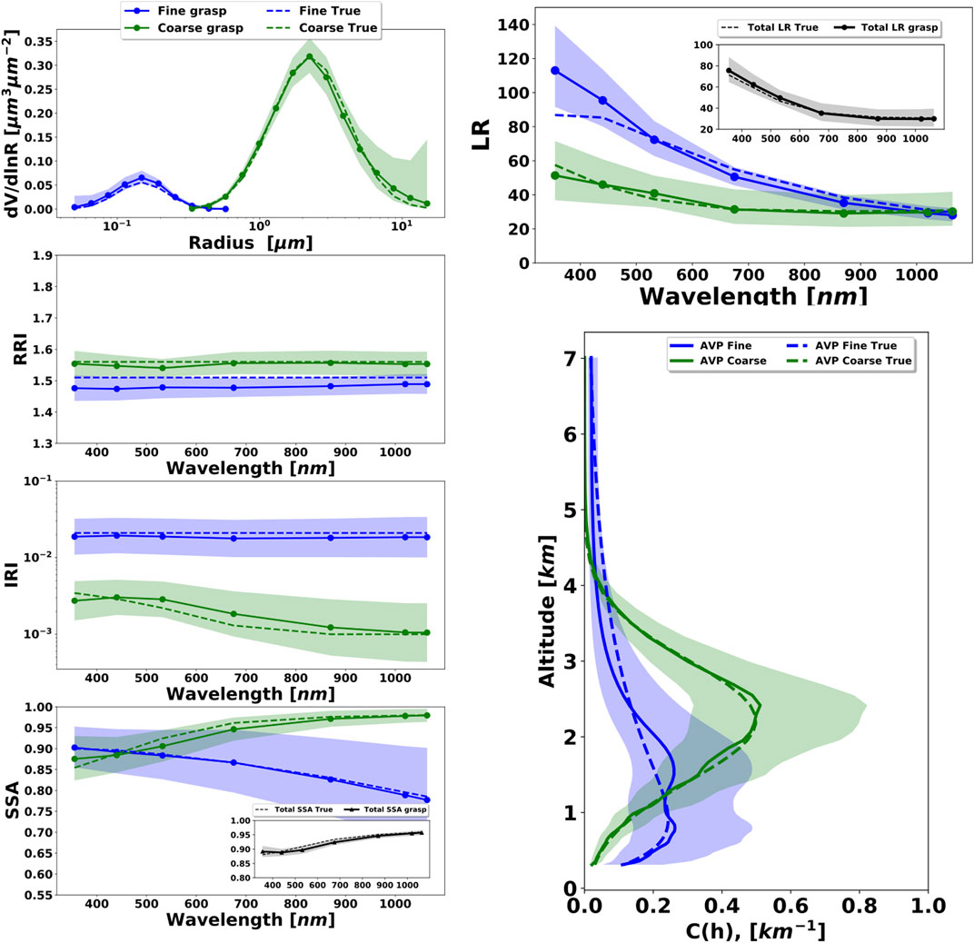
FIGURE 10. An example of GaRRLiC/GRASP retrieval columnar and vertical aerosol properties from a combination of ground-based radiometer and multi-wavelength lidar, LR denotes lidar ratio, RRI and IRI denote real and imaginary refractive indices respectively.

While the original GARRLiC scheme was limited to the specific observational set of multi-wavelength elastic scattering lidar together with AERONET-like sun/sky-radiometer observations, the area of GRASP application was significantly extended during last years and now covers a variety of active and vertically resolved observations that can be processed. For example, at present GRASP can be applied for interpretation of such vertical observations of atmosphere as profiles of extinction, backscatter, normalized elastic and inelastic lidar signals, profiles of volume and particle depolarization. In addition, a possibility of lidar only retrieval was introduced in GRASP together with several technical retrieval details improving processing of vertically resolved observations (Lopatin et al., 2021).

Thus, at present GRASP allows simulation and inversion of point or vertical observations of the profiles of backscattering, extinction, 6 elements of scattering matrix. In addition, several characteristics that are simple functions of the above scattering characteristics were introduced as a potential input data for GRASP. Specifically, both the elastic and inelastic lidar measurements can be inverted by GRASP. The lidar equation for ground-based observations is realized as the following:

$\mathit{L}\left(\lambda \mathit{,h}\right)=A\left(\lambda \right)\beta \left(\lambda ,h\right)\exp \left(-2{\displaystyle \underset{Z_{\min }}{\overset{Z\left(h\right)}{\int }}\sigma \left(\lambda ,z\right)dz}\right),$(4.3.1)

where $\sigma \left(\lambda ,h\right)$ denote extinction and $\beta \left(\lambda ,h\right)$ backscattering profiles. The extinction profile includes aerosol, molecular scattering and gaseous absorption components $\sigma \left(\lambda ,h\right)={\sigma }_a+{\sigma }_m+{\sigma }_g$ and backscattering includes aerosol and molecular components $\beta \left(\lambda ,h\right)={\beta }_a+{\beta }_{m\text{'}}$, $A\left(\lambda \right)$ is the instrumental constant, $z\left(h\right)$ is lidar path related with the atmospheric altitudes of target h, ground level h_BOA and zenith angle of lidar inclination ${\Theta }_L$ as $z\left(h\right)=\frac{h-h_{BOA}}{\cos \left({\Theta }_L\right)}$. Here both backscattering and extinction profiles depend of aerosol properties. The ambiguity in separation of the backscattering by the layer and extinction of the lidar signal by underlying layers is considered as the key challenge in the interpretation of elastic lidar signals. The lidar systems using inelastic scattering address that ambiguity by measuring the following signal:

$L_{inel}\left(\lambda \text{,}h\right)=A\left(\lambda ,\lambda \prime \right){\beta }_{inel}\left(\lambda ,h\right)\exp \left(-{\displaystyle \underset{Z_{\min }}{\overset{Z\left(h\right)}{\int }}\left(\sigma \left(\lambda \prime ,z\right)+\sigma \left(\lambda ,z\right)\right)dz}\right)$(4.3.2)

where scattering, $\lambda \prime$ – wavelength of exciting impulse that triggers inelastic backscatter at wavelength $\lambda$, ${\beta }_{inel}\left(\lambda ,h\right)$ inelastic backscattering of atmosphere, $A\left(\lambda ,\lambda \prime \right)$ is known calibration constant. The shift $\lambda \prime \to \lambda$ in inelastic backscattering ${\beta }_{inel}\left(\lambda ,h\right)$ could be a result of gaseous molecules emission frequency shifts due rotations and vibrations of molecules and can be rather accurately estimated based on known characteristics of emitted lidar impulse and atmospheric gases. Therefore, neglecting the differences in aerosol extinction at $\lambda \prime$ and $\lambda$,${\sigma }_a\left(\lambda ,h\right)$ can be considered as the only fully unknown characteristic in Eq. 4.3.2 and can be obtained from $L_{inel}\left(\lambda \text{,}h\right)$ by rather straightforward transformations. The measurements of such advanced lidar systems as HSRL are usually converted to the backscatter $\beta \dots \left(\lambda ,h\right)$ and extinction profiles $\sigma \dots \left(\lambda ,h\right)$ (Hair et al., 2008; Rogers et al., 2009, etc.) that can be used as an input to GRASP algorithm for conducting a full aerosol retrieval.

Another characteristic measured by advanced lidars with polarimetric capabilities is the profile of volume and aerosol particle depolarization. The profile of particle depolarization can be estimated from the ratio of lidar returns $L_{\perp }$ and $L_{\parallel }$ obtained with from emitted polarized light beams as following (Freudenthaler et al., 2009):

$\delta =\frac{L_{\perp }\left(\lambda \text{,}h\right)}{L_{\parallel }\left(\lambda \text{,}h\right)}=\frac{{\beta }_{\perp }\left(\lambda \text{,}h\right)}{{\beta }_{\parallel }\left(\lambda \text{,}h\right)}=\frac{P_{11}\left(\lambda ,180\mathrm{°},\mathit{h}\right)-P_{22}\left(\lambda ,180\mathrm{°},h\right)}{P_{11}\left(\lambda ,180\mathrm{°},h\right)+P_{22}\left(\lambda ,180\mathrm{°},h\right)},$(4.3.3)

where the subscripts “$\perp$” and “$\parallel$” indicate cross- and co-polarized components correspondingly. Both profiles of aerosol and atmospheric volume depolarization ratio can be used for GRASP.

Thus, diverse vertically resolved observations discussed above from a single instrument or in a combination with other observations (e.g., a passive instrument) can be inverted by GRASP. The number and type of aerosol parameters retrieved depend on a chosen configuration of employed aerosol forward model (see Theory of Multi-Term LSM Inversion) and a priori constraints that should be chosen in accordance with the information content of inverted data. For example, if only observations of a single wavelength lidar are inverted, only profile of one aerosol component can be retrieved using a priori assumptions about most of other aerosol characteristics. In case of inversion of observation from multi-wavelength advanced lidar system, a number of parameters and scope of retrieved aerosol information can be significantly extended. For example, Lopatin et al. (2021) demonstrated simultaneous retrieval of four profiles of different aerosol components from such data (aerosol was modeled using Eq 3.10, 3.11). Lopatin et al. (2021) provided more detailed discussion of GRASP applications to inversion of vertically resolved observations and numerous illustrations.

4.4 Satellite and Airborne Passive Observations

One of the original motivations for initializing GRASP developments was an idea of creating enhanced retrieval of aerosol from satellite observations by multi-angle polarimeter such as POLDER. In fact, numerous theoretical and practical studies have concluded that polarimetry is an approach that can provide an accurate characterization of aerosols with the detail and precision sufficient for many important applications (Mishchenko et al., 1997; Mishchenko and Travis, 1997; Hasekamp and Landgraf, 2005; Hasekamp and Landgraf, 2007; Kokhanovsky et al., 2010; Knobelspiesse et al., 2012). On the other hand, as discussed by Dubovik et al. (2019), the interpretation of multi-angular multi-spectral polarimetric (MAP) data is quite challenging from the fundamental point of view. Indeed, polarimetry is highly sensitive to a large number of atmospheric parameters, and accounting adequately for all these sensitivities in the retrieval algorithm is very demanding, especially in the satellite applications where large volumes of data need to be processed with a minimal delay, and for quite a long time there were no available operational MAP product demonstrating the practical advantages of MAP retrieval. In these regards, GRASP was adapting AERONET retrieval methodology and, in difference with conventional look-up-table (LUT approaches) attempted highly advanced statistically optimized fitting of satellite data implementing rigorous search for the solution in a continuous space of solutions. Such approaches are considered as the most promising for satellite retrieval and with some technical differences are deployed in other algorithms of new generations developed for interpretation of MAP observations (Hasekamp and Landgraf, 2007; Hasekamp et al., 2019; Fu et al., 2020; Dubovik et al., 2011; Xu et al., 2016; Xu et al., 2017, etc.). The challenges of realizing such state-of-the-art algorithms lie in the fundamental difficulties to adapt them optimally to the high sensitivities of MAP instruments and in specific technical issues, such as, a need of significantly more computational time than LUT algorithms to simulate the satellite signal and the Jacobian derivatives matrices online. In these regards, the developed structure of GRASP algorithm allows realizing rigorous inversion of MAP satellite observations. In addition, the GRASP software was extensively optimized to reduce time of calculation and adapted to practical application to real satellite observations.

At present, 18 months of POLDER-1 and -2 and 9 years of POLDER-3 observations have been processed and several versions of the retrieval product have been archived at the AERIS/ICARE Data and Services Center (http://www.icare.univ-lille1.fr) and GRASP-OPEN site (https://www.grasp-open.com). For POLDER, GRASP utilizes radiance and polarization observations from all available spectral channels with minor gaseous absorption: 5 and 6 channels for POLDER-1 and -2, and POLDER-3, correspondingly and 3 polarized radiances spectral channels for all instruments. The retrieval uses a unique global set of constraints (no location-specific assumptions) and a single initial guess globally. The radiative transfer computations accounting for multiple interactions of the scattered solar light in the atmosphere are performed on-line. All GRASP retrievals were performed at POLDER native resolution POLDER-1 and -2 at ∼7 km and POLDER-3 at ∼6 km. In the saved data archives, the original POLDER/GRASP retrievals are stored at Level-1, Level-2 and -3 products and are publicly available in the form of daily, monthly, seasonal, yearly and climatological datasets. The Level-2 data contain full resolution data filtered following the established quality criteria. Level 3 data is aggregated into a 0.1° and 1° grid box using the sinusoidal projection from Level-2 data.

GRASP allows a variety of different possibilities on modeling aerosol scattering, surface reflectance and implementing atmospheric RT calculations and due to various reasons several different configurations of the atmospheric forward model were used to generate aerosol products. For example, the full POLDER-3/PARASOL data archive was processed by GRASP using the three following retrieval configurations: POLDER-3/GRASP «optimized», «high-precision» and «models». The observations of POLDER-1 and -2, at present, were processed using only a single GRASP/Models approach. The «optimized» and «high-precision» differ only by the precision of the RT calculations, while they use the same aerosol model driven by aerosol size distribution, spectral values of complex index of refraction, fraction of spherical particles and the aerosol scale height (Dubovik et al., 2011). The «models» approach uses the assumption of an external mixture of several aerosol components (see Eq 3.10‐3.11) and directly retrieved parameters include aerosol concentrations and a scale height. In addition, recently POLDER-3/GRASP aerosol product has been generated using “component” approach (Li et al., 2019; Li et al., 2020a; Li et al., 2020b). This approach retrieves the size resolved fractions of aerosol components representing the different composition species, such as black carbon, brown carbon, fine/coarse mode non-absorbing soluble and insoluble, coarse mode absorbing and aerosol water. The retrieved fractions drive the aerosol spectral index of refraction in modeling of atmospheric radiances. Figure 11 illustrates the climatology of aerosol component columnar mass concentration derived from POLDER-3 over East Asia region by the GRASP/Component algorithm.

FIGURE 11

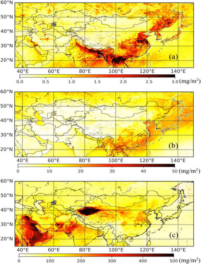
FIGURE 11. Climatology of aerosol component columnar mass concentration derived from POLDER-3 over East-Asia by the GRASP/Component approach: (A) fine mode black carbon, (B) fine mode brown carbon, (C) coarse mode mineral dust.

Independently of which aerosol model approach all retrieval data products contain the aerosol main aerosol characteristics including spectral aerosol optical depth (AOD), aerosol absorption optical depth (AAOD) and single scattering albedo (SSA) as well as Ångström exponent (AE), spectral fine mode AOD (AODF) and coarse mode AOD (AODC). Figure 12 illustrate the climatology of these parameters.

FIGURE 12

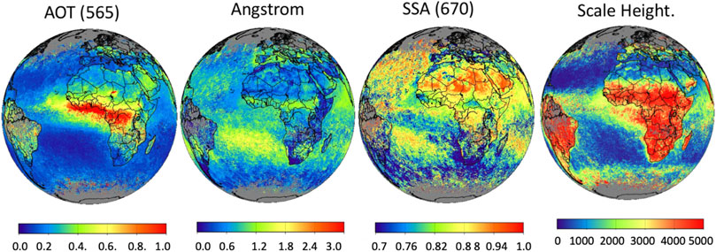
FIGURE 12. Climatological values of AOD (565), Angstrom exponent, SSA(670) and scale height for winter 2009 provided by POLDER-3/GRASP optimized product.

The main aerosol POLDER-3/GRASP products including AOD, AE, AODF, AODC, SSA and AAOD were extensively evaluated using validations against AERONET and comparisons with the original POLDER algorithm (PARASOL/Operational), and MODIS Collection 6 aerosol products. For example, Schutgens et al. (2021) have evaluated GRASP/Models Level3 1-degree SSA against AERONET and compared with other satellite SSA products. The studies recognized GRASP/ Models as one of reliable and most extensive data SSA set. Chen et al. (2020) have conducted the detailed validation of Level 3 0.1 degree products. The studies have shown that the POLDER-3/GRASP retrieval provided reliable aerosol products. Specifically, POLDER-3/GRASP spectral products including AOD for six wavelengths in the range 443–1,020 nm agree well with the AERONET AOD measurements, e.g., for POLDER-3/Models AOD correlation coefficients R are ≥0.86 over land and ≥0.94 over ocean with BIAS not exceeding 0.01 over land and 0.02 over ocean for all wavelengths. The upper panel of Figure 13 demonstrates the correlations of satellite AOD with AERONET for several selected wavelengths.

FIGURE 13

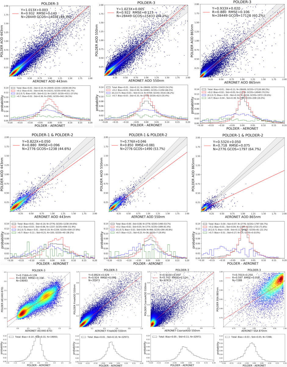
FIGURE 13. The illustrations of the POLDER/GRASP product comparisons with AERONET data. Upper panel: the correlations of POLDER-3/Models AOD with AERONET for several selected wavelengths (440, 550, 870 nm). Middle panel: the correlations of POLDER-1,2/GRASP AOD with AERONET for several selected wavelengths (440, 550, 870 nm). Lower panel: the correlations of the detailed aerosol parameters retrieved by POLDER-3/GRASP/HP product, from left to right: AE, AODF(550), AODC(550), SSA(865).

The data from POLDER-1 and -2/GRASP retrievals were not included in the analysis by Chen et al. (2020), while the limited comparisons are shown in middle panel of Figure 13 demonstrate that the quality of the POLDER-1 and -2/GRASP retrievals are expected to be close to those of POLDER-3/GRASP retrievals.

The comparisons with MODIS aerosol products showed that the POLDER-3/GRASP AOD retrievals are very coherent with popular MODIS data while also exhibit some important advancements. For example, POLDER-3/GRASP retrievals provide more reliable detailed aerosol parameters such as AE, AODF and AODC especially over land and such parameters as SSA and AAOD that are generally not available from MODIS-like instruments. The validation of POLDER-3/GRASP products by Chen et al. (2020) showed a robust correlation of the retrieved SSA and AAOD spectral values with AERONET (440–1,020 nm), correlations increase for the retrievals corresponding to the events with higher AOD. For AAOD retrievals overall the BIAS did not exceed 0.01, suggesting that POLDER-3/GRASP products can be used for making global estimations of AAOD at such level of uncertainty. The lower panel of Figure 13 demonstrates the correlations of the detailed POLDER-3/GRASP/HP products. The detailed discussion can be found in the study by Chen et al. (2020).

One key finding of Chen et al. (2020) analysis is that the best retrieval of total AOD is provided by the simplest approach (GRASP/Models) in which the retrieval is restrained to a superposition of predefined aerosol components, significantly reducing the number of free parameters for retrieval. The AOD retrieved from more complex GRASP/HP and GRASP/Optimized approaches over land has notable bias (∼0.06–0.07 at 500). In these regards, the GRASP/Component [that was not considered by Chen et al. (2020)] provided apparently overall the most coherent total and detailed aerosol properties. Indeed, the validation by Zhang et al. (2021) of GRASP/Component POLDER-3 products against AERONET showed that total AOD from GRASP/Component is close in accuracy to GRASP/Models and higher in accuracy than AOD form GRASP/HP and GRASP/Optimized. Also, the accuracy of most of detailed aerosol products (AOF, AOC, AE) from GRASP/Component approach is overall higher or close to that of best results of GRASP/HP and GRASP/Optimized. For example, Figure 17 illustrates results for AOD, AODF, AODC and AE over land that can be compared in Figures 13, 14.

FIGURE 14

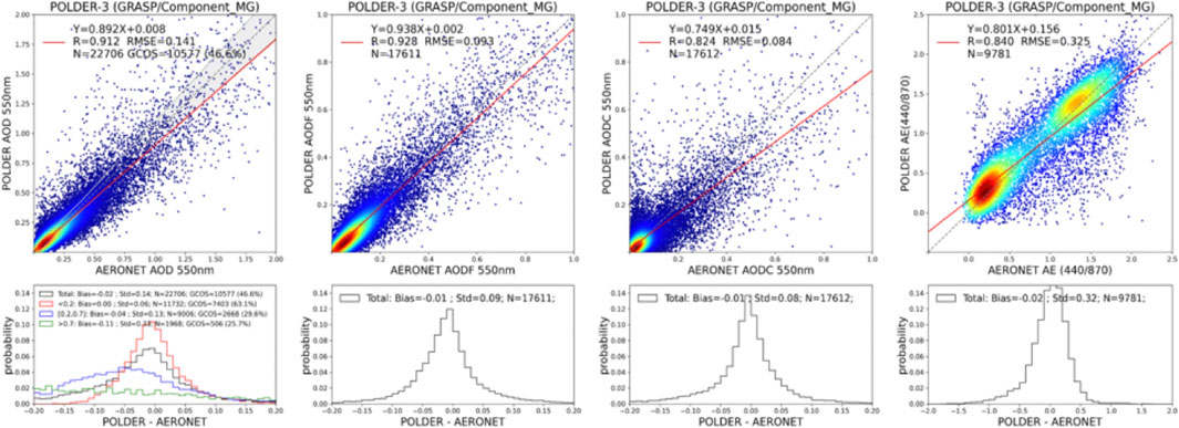
FIGURE 14. The correlations of the detailed aerosol parameters retrieved by POLDER-3/GRASP/Component product, from left to right: AOD(550), AODF(550), AODC(550), AE.

Evidently, that future efforts on improving the GRASP retrieval will be aimed at achieving accurate retrievals within one approach, however the situation also reveals the challenge of developing a unique approach that can provide a retrieval of all parameters with highest accuracy from MAP observations. Indeed, multi-angular polarimetric observations have sensitivity to different aerosol properties, and therefore the MAP algorithms tend to be designed for the retrieval of large number of parameters, while in the situations with low aerosol presence the information from observations may not be sufficient to retrieve all parameters reliably. Moreover, POLDER like MAP observations have high potential for essentially helping to improve extensive monitoring air quality parameter that are vital for many evaluating the dynamic of environment. For example, Wei et al. (2020) demonstrated higher capacity of POLDER product than single-view MODIS data for characterization of PM2.5 from space and Wei et al. (2021) presented a methodology of POLDER/GRASP products for deriving PM10 the characteristics that is generally even more difficult to obtain from remote sensing than PM2.5. Moreover, MAP and specifically POLDER/GRASP data provide were used as additional constraints for improving global emissions of the atmospheric components in chemical transport models (e.g., Chen et al., 2018; Chen et al., 2019; Elguindi et al., 2020). This supports the highly promising concept of synergizing satellite with available modeled information for advancing satellite remote sensing.

In all above processings, the underlying surface reflectance was retrieved simultaneously with the aerosol properties and the detailed BRDF (Bi-directional Reflectance Distribution Function) and BPDF (Bi-directional Polarization Distribution Function) of ocean and land surfaces were derived. Specifically, the parameters of “Ross-Li model” BRDF and Maignan et al. (2009) BPDF models were retrieved over land. Figure 15 demonstrates the climatological surface reflectance properties retrieved from POLDER-3.

FIGURE 15

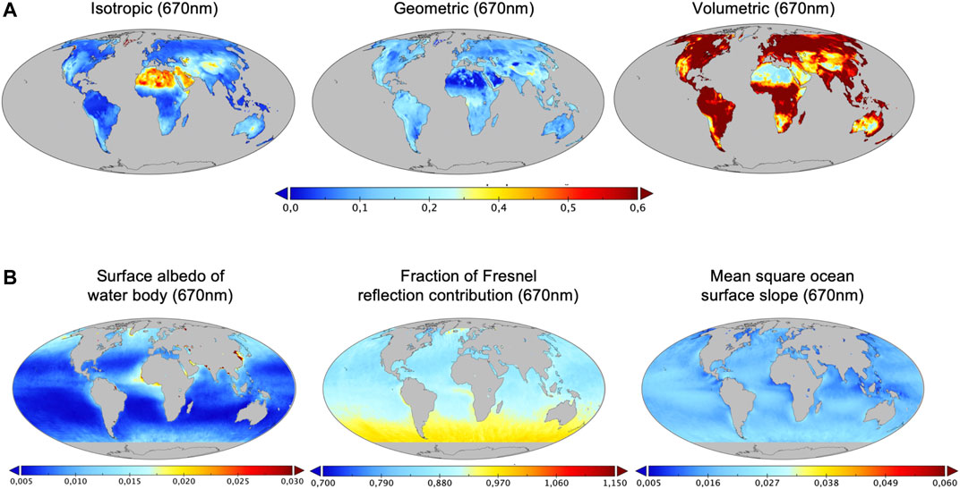
FIGURE 15. Climatological values (9 years averages) of surface reflectance properties retrieved from POLDER-3. (A): the land BRDF parameters. (B): the ocean surface reflectance parameters.

The preliminary validations of POLDER surface reflectance show a generally good agreement with other surface products as those from MODIS, especially for such general parameters as surface albedo. At the same time, for detailed BRDF properties some differences are obvious for the Ross-Li model parameter related with angular anisotropy of surface BRDF. For example, Figure 16 illustrates the correlations of three Ross-Li model BRDF parameters provided by POLDER-3/GRASP and retrieved by MODIS. The correlations for 2-nd and 3-rd parameters are significantly lower than for the first one. This can be explained by high sensitivity of both POLDER and MODIS observations to the total reflectance of the land surface, while the sensitivity to the BRDF anisotropy, driven by 2nd and 3rd BRDF parameters, is evidently higher for the multi-viewing POLDER than for single-view MODIS measurements.

FIGURE 16

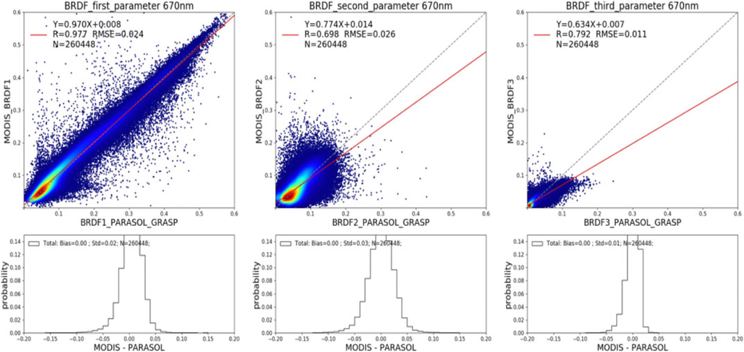
FIGURE 16. The correlations of the land BRDF monthly average parameters retrieved for September 2008 from POLDER-3 and MODIS.

The reflective properties of ocean surface are modeled analogously to earlier developments (Deuzé et al., 2001; Herman et al., 2005; Tanré et al., 2011). The Fresnel’s reflection on the agitated sea surface is considered by using the Cox and Munk model (Cox and Munk, 1954). The water leaving radiance term and the white cap reflection are taken into account for by Lambertian unpolarized reflectances (Voss et al., 2007). The whitecaps reflectance are dependent on the wind speed at sea surface (Koepke 1984). The seawater reflectance at short wavelengths is not negligible and depends on the properties of the oceanic waters. Thus, in POLDER-3/GRASP, the magnitude of seawater reflectance at each wavelength and the wind speed could be retrieved together with aerosol. The lower panel of Figure 15 illustrates climatology of ocean surface parameters retrieved from POLDER-3. More illustrations of the chlorophyll, water leaving radiances and wind speed retrievals and their comparison with MODIS results and ECMWF reanalysis can be found in the paper by Frouin et al. (2019). The detailed analysis of both land and ocean surface reflectance properties provided by POLDER/GRASP are ongoing and expected to be discussed in the separate paper.

It is also important to emphasize that POLDER-3/GRASP retrievals are based on rigorous optimized inversion that searches for statistically optimized fitting in a continuous space of solution without using widely used Look-up-Tables, unlike as most of the conventional satellite retrievals. As a result, POLDER/GRASP aerosol and surface reflectance products are globally-consistent based on exactly the same aerosol modeling approach over land and ocean, unique set of a priori constraints and initial guess, while retrieving surface reflectance properties simultaneously with aerosol. As discussed by more in Dubovik et al. (2019) the similar type of approaches is expected to become common and evolve further in the coming era of multiple MAP instruments. In these regards, there are several GRASP based developments for the future polarimetric mission. For example, an operational aerosol retrieval algorithm for future 3MI/EPS-SG polarimeter (Fougnie et al., 2019) has been developed using GRASP (Marbach et al., 2020). There are also some efforts to adapt GRASP for processing the observations by the future DPC, Aerosol-UA, HARP2 missions. For example, Figure 17 illustrates the application of the GRASP algorithm for processing AirHARP (airborne Hyper Angular Rainbow Polarimeter) observations made during the NASA ACEPOL 2017 campaign (Puthukkudy et al., 2020a). GRASP retrieved AOD using the AirHARP data is validated using the collocated AERONET and HSRL2 measurements. Figure 17C shows a good agreement of GRASP AirHARP retrieved AOD with the collocated AERONET AOD observation with a maximum bias of -0.009 and mean absolute error of 0.015 at 870 nm band. Comparison of GRASP retrieved AOD with measurement of HSRL2 lidar for a forest fire smoke plume shows good correlation and agreement with a correlation coefficient of 0.940 at 532 nm (see Figure 17D). Furthermore, preliminary aerosol retrievals based on the HARP CubeSat data using the GRASP was presented at the AGU Fall meeting 2020 (Puthukkudy et al., 2020b). There are also successful GRASP developments for SGLI/GICOM-C and MISR observations (Fuertes et al., 2020).

FIGURE 17

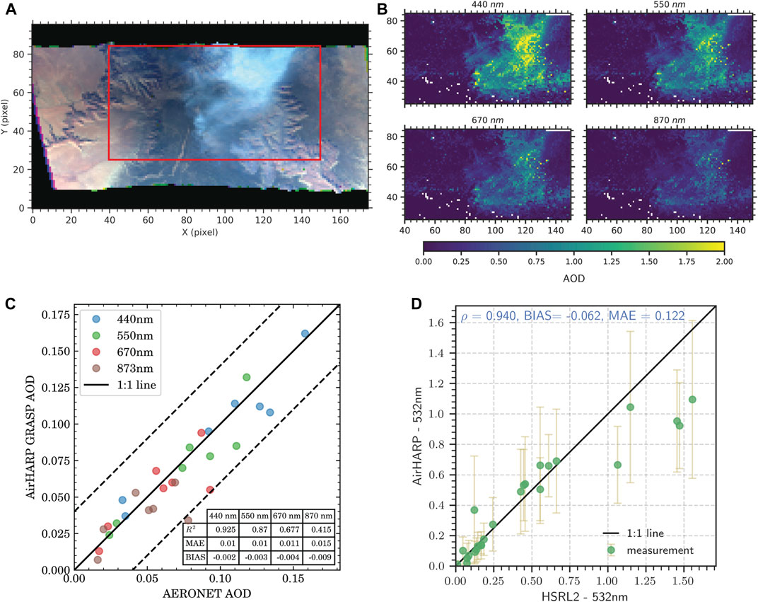
FIGURE 17. The application of GRASP algorithm for processing AirHARP observations during the ACEPOL 2017 campaign (Puthukkudy et al., 2020a): (A) RGB image of a forest fire smoke scene captured on 27th October 2017 18:16 UTC; (B) AOD map retrieved for different spectral bands data for the pixels shown in the red rectangle; (C) Comparison of AirHARP-GRASP retrieved AOD with collocated AERONET; (D) Scatterplot of the AOD measured by HSRL2 with GRASP-AirHARP retrieved AOD for a smoke plume on 7th November 2017 19:31 UTC. [Adapted version of the plots originally published in Puthukkudy et al. (2020b), CC BY 4.0].

GRASP approach has also been successfully applied to several single-view satellite radiometers. For example, GRASP has been used to process 10 years (2002–2012) of MERIS (MEdium Resolution Imaging Spectrometer). MERIS is an imaging spectrometer operated from Envisat satellite platform that scanned the Earth’s surface by the so-called push-broom method. Linear CCD arrays provided spatial sampling in the across-track direction, with the satellite’s motion provided scanning in the along-track direction (Rast et al., 1999). MERIS/GRASP retrieval provided aerosol and surface reflectance retrieval product at 8 used channels 413, 443, 490, 510, 560, 665, 760 and 870 nm. The data were inverted at resolution of 10 km in cloud-free conditions as determined by original MERIS cloud-mask algorithm at latitudes below 60 degrees north and south. The retrieval of aerosol and surface properties is conducted simultaneously. An external mixture (see Eq. 4.3.3) of four aerosol components was used for modeling aerosol. The surface BRDF as well as general retrieval approach was similar to the POLDER/GRASP processing e.g., multi-pixel concept was applied. The full list of the retrieved parameters, as well as, Level 2 and Level 3 products of all derived parameters are available at GRASP-OPEN website (https://www.grasp-open.com).

The MERIS/GRASP products were validated against AERONET and compared to other satellite products. The analysis has shown that MERIS/GRASP retrievals provided robust and reasonably accurate results. For example, as illustrated in Figure 18 MERIS/GRASP spatial distribution of aerosol hot spots agrees qualitatively well with POLDER/GRASP products. Figure 19 shows the global correlations of MERIS/GRASP AOD(560) with AERONET data. The correlations coefficients are ∼0.76 over land and ∼0.84 (over ocean) with RMSE of 0.155 over land and ∼0.06 over ocean. There is a rather small systematic bias of ∼0.03 over ocean. However, over land the bias significantly higher: ∼0.09. The origin of such high bias over land is being investigated and expected to be addressed in ongoing efforts on updating MERIS/GRASP product. The land surface products are generally in good agreement with the products from other satellite instruments, such as MODIS and POLDER. The lower part of Figure 19 illustrates the global comparisons of retrieved DHR (Direct Hemispheric Reflectance) with values provided by MODIS.

FIGURE 18

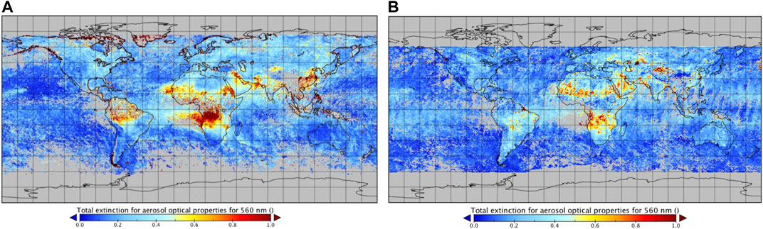
FIGURE 18. The AOD(560) retrieved by POLDER/GRASP (A) and MERIS/GRASP (B) for September 2008.

FIGURE 19

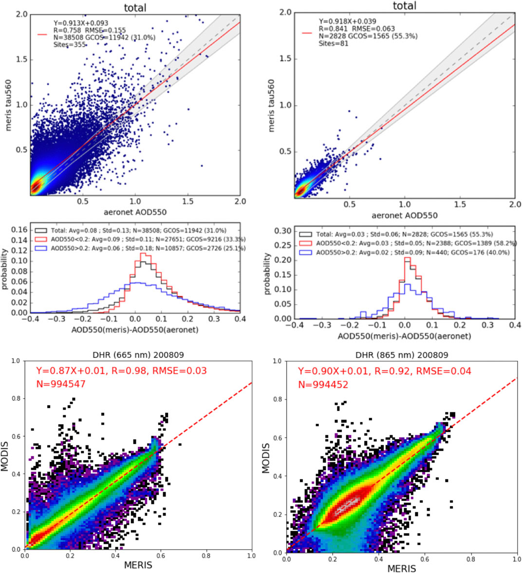
FIGURE 19. The illustration of MERIS/GRASP validation results globally. The upper panel: the correlations of MERIS/Models AOD(560) with AERONET globally for entire MERIS archive: Left - over land, Right – over ocean. The lower panel: The correlations of DHR (Direct Hemispheric Reflectance) retrieved by MERIS/GRASP and MODIS over land globally for September 2008, for several selected wavelengths (665 and 865 nm).

The GRASP is been also applied to other single or dual-view radiometers. For example, at present there are several ingoing GRASP based developments of algorithms and retrieval products for Sentinel-3, Sentinel-4 and Sentinel-S5P, VENUS, PRISMA, HIMAWARI, SGLI-2, etc.

It should be noted that while the estimations of the retrieval errors were not generated as a part of POLDER/GRASP and MERIS/GRASP products, but were included in all new and recent developments. For example, Figure 20 illustrates the result of the numerical tests, were the AOD was retrieved from synthetic observation of S5P/GRASP AOD simulated over Banizoumbou AERONET site (the random noise of ∼3% was added to the simulations). It can be seen that the error estimates of satellite data obtained based on Eq 2.3.1–Eq 2.3.7 and denoted by the error bars agree well with assumed data. The detailed discussion on performance of GRASP error estimation concept is provided by Herrera et al. (2020).

FIGURE 20

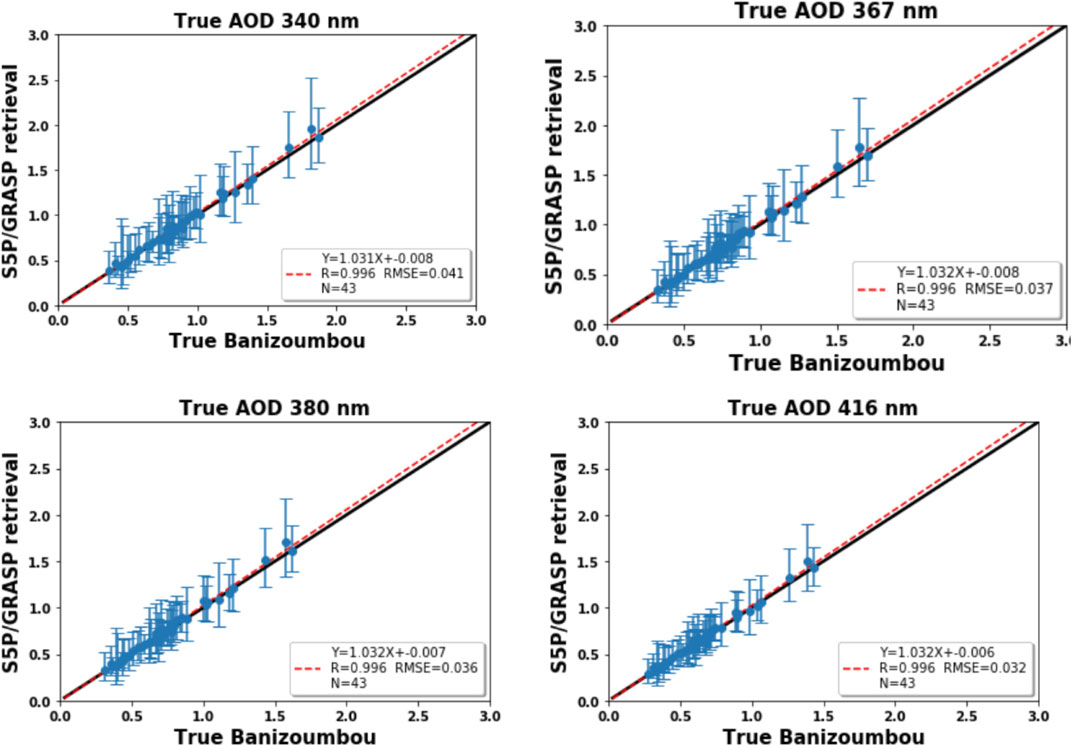
FIGURE 20. The correlations of S5P/GRASP AOD retrievals and their error estimates for the numerical tests, where the AOD was retrieved from synthetic observations of S5P/GRASP AOD simulated over Banizoumbou AERONET site (the random noise of ∼3% was added to the simulations) for Summer 2019.

4.5 Synergetic Retrievals and Other Diverse GRASP Applications

As described above the GRASP is a versatile algorithm that have been already used in a wide variety of applications including diverse passive and active ground-based and satellite observations as well as in situ and laboratory observations. Figure 21 shows the overview diagram of GRASP applications. The several key and mature applications have been described above in this section. At the same time, there are some other different but relevant applications of GRASP that have been realized by different studies. For example, GRASP has been used for processing observations by moon-light sky-camera by Roman et al. (2017), for utilization with the ceilometers by Roman et al. (2018), for processing sun/sky aureole measurements by Torres and Fuertes (2020), etc.

FIGURE 21

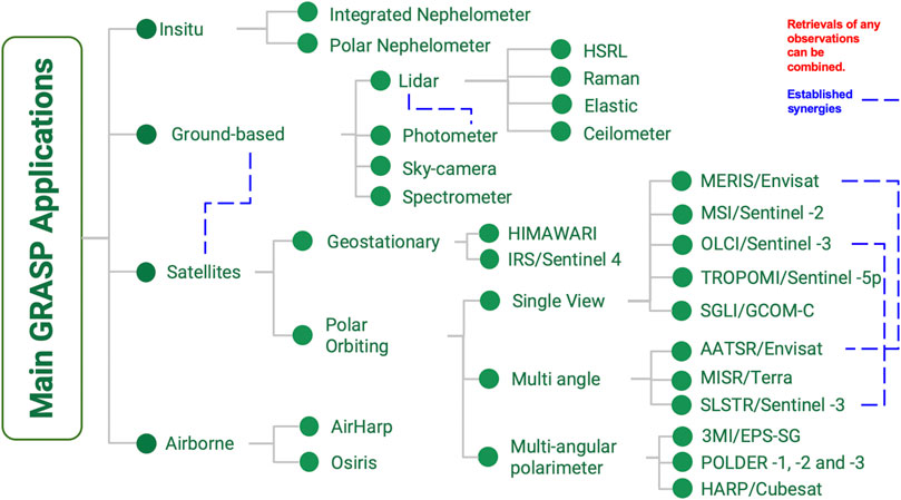
FIGURE 21. The diagram illustrating current application of GRASP code.

It is important to note that the full compatibility of all retrievals inside of GRASP is fundamental base for the developments of diverse synergetic retrievals. Indeed, in a case if even very different observations of similar natural event are available then the interpretation of these observations by GRASP can be combined together in a single synergetic retrieval. It can be mentioned here that the DIVA (Demonstration of an Integrated approach for the Validation and exploitation of Atmospheric missions) platform has been develop to promote and simplify practical use of the GRASP synergetic capabilities (Fuertes et al., 2019). The system operates in computer cloud and contains loaded data from ground and space observation that can be easily used for the exploration of new retrieval possibilities such as the joint retrieval of the gas aerosol properties showed in Ground-Based Passive Observations or the joint inversion of ground-based radiometer and lidar observations discussed in Ground-Based Active Observation and Synergy With Passive Observations is only one example of such synergy. Similar approach is also being developed for synergetic processing of passive and active satellite observations. For example, GRASP based approach has been used in extensive numerical tests in frame of ongoing NASA Aerosol and Cloud, Convection and Precipitation (ACCP) study. The ACCP initiative considers deployment of coordinated observations by passive (polarimeter, spectrometer, microwave radiometer) and active (lidar and radar) sensors (https://science.nasa.gov/earth-science/decadal-accp). Figure 22 illustrates the application of a GRASP-based testbed realized by Espinosa W. R. et al. (2019) for exploring the capabilities of synergistic passive and active remote sensing using a combination of multi-angular polarimeter and lidar observations considered in ACCP for future deployment. The aerosol retrieval displayed in Figure 22 demonstrates that a retrieval using total and polarimetric radiances paired with HSRL lidar profiles can yield accurate, mode-resolved extinction profiles in relatively complex scenes. Retrievals of such quality are unachievable with just lidar or polarimeter data alone.

FIGURE 22

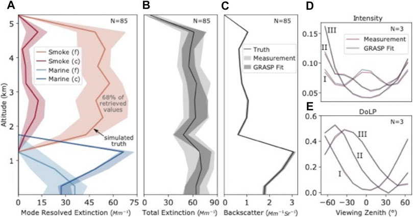
FIGURE 22. The results of synthetic tests of aerosol retrieval using a combination of polarimeter and HSRL lidar satellite data from a simulated scene containing a bimodal smoke layer above a bimodal marine aerosol. Panel (A) illustrates GRASP’s ability to retrieve the fine (f) and coarse (c) mode extinction contributions in each of the two layers over N = 85 tests under various polarimeter viewing geometries and instantiations of measurement noise. Panels (B) and (C) show the corresponding 1σ distribution of simulated measurements and the corresponding GRASP fits for total aerosol extinction and backscatter, respectively. Panels (D) and (E) show the simulated polarimeter measurements and fits for 3 of the 85 tested geometries: I (θ_s = 19°,φ = 85°), II (θ_s = 36°,φ = 35°) and III (θ_s = 58°,φ = 35°). Across all 85 tests, the retrieved AOD, AODF and SSA had RMS errors of 0.003, 0.005 and 0.003, respectively.

When only using lidar measurements for deriving aerosol properties, a different retrieval strategy can be adopted with GRASP. Instead of fully and independently retrieving particle microphysical and intensive optical properties, multichannel lidar measurements can be used to quantify the contribution of different aerosol components, that can be considered as aerosol “types”, to the vertical concentration profile of aerosols. The development of this approach in GRASP is also discussed in detailed by Lopatin et al. (2021). Each aerosol type may be assumed to be characterized by climatological size distributions and refractive indexes, which can also be used to infer effective aerosol properties for the mixture of aerosol types. This is the approach adopted by Cuesta (2021) to exploit the measurements of the future satellite mission ACCP that will deploy an advanced lidar payload providing for the first time multiwavelength, multipolarisation and high spectral resolution capabilities. This method is illustrated in Figure 23 for an example of vertical distribution of five different aerosol types (the pseudo-reality in Figure 23A) and forward calculations of lidar measurements for 3 wavelengths (355 nm, 532 nm and 1,064 nm) with depolarization capabilities for each of them and HSRL-derived particle backscatter and extinction profiles measured in the UV and visible channels (Figures 23B–E). This numerical application also considers instrumental noise according to the ACCP lidar payload, a vertical resolution of 500 m and 50 km horizontal averaging, as well as perturbations of the size distributions and refractive indexes with respect to the climatological values of each aerosol type. The joint and simultaneous fit of the 8 lidar-derived profiles allows the retrieval of the profiles of the abundances of the 5 aerosol types (Figure 23F) with almost negligible error with respect to the supposed true (Figure 23A).

FIGURE 23

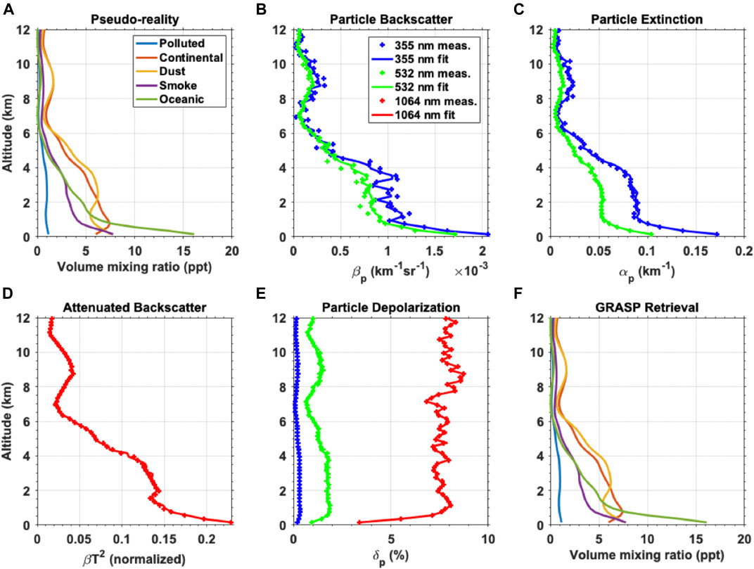
FIGURE 23. Multiwavelength high spectral resolution spaceborne lidar retrieval of the aerosol concentration profile as a function of aerosol type based on the GRASP approach. (A) Pseudo-reality of aerosol concentration profiles for 5 selected types. Lidar measurements calculated with the GRASP forward model and adding random noise for measured (crosses) and fitted (plain lines) profiles of (B) particle backscatter, (C) particle extinction, (D) attenuated total backscatter and (E) particle depolarization ratio. (F) Retrieved concentration profiles from GRASP inversion quantified for the 5 aerosol types. Forward calculations of lidar-derived profiles are provided for the available wavelengths (355 nm in blue, 532 nm in green and 1,064 nm in red) with noise equivalent to night-time conditions, vertical resolution of 500 m and horizontal resolution of 50 km, as well as adding perturbations in the size distribution and complex refractive index of each aerosol type with respect to the fixed aerosols properties used in the inversion.

Also, it has been shown that multi-pixel approach realized in GRASP is eventually useful for enhanced synergetic processing of ground-based observations. It was demonstrated that this principle can be rather efficient for combining non-coincident but close in time observations, e.g., day- and night-ground-based measurements. For example, Lopatin et al. (2021) demonstrated that combining the daytime radiometric and photometric data with nighttime observations by elastic or inelastic lidars and radiosondes could be achieved. As illustrated in the scheme shown in Figure 24 in such synergetic approach the aerosol information from the morning and evening observations helps to constrain the retrieval during the night. The same approach was used by Parajuli et al. (2020) for generating aerosol climatology base on synergetic processing of daytime AERONET observation with day and night time observation by MPL lidar. Somewhat similar but simpler strategy was used by Benavent-Oltra et al. (2019) for combining sun–sky radiometric daytime measurements with nighttime lidar and lunar photometry observations.

FIGURE 24

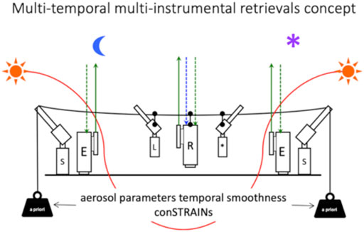
FIGURE 24. The illustration of synergy processing of collocated but not fully coincident ground-based observations using smoothness a priori constraints on temporal variability of aerosol in frame of multi-pixel retrieval approach by Dubovik et al. (2011).

In addition, GRASP can be applied for synergetic aerosol and surface properties retrieval from coordinated ground-based and satellite observations. Indeed, the set of observations containing both satellite and ground-based measurements has substantial sensitivity to both contributions from surface (especially over land) and aerosols that is not always a case for satellite only or ground-based only data. The advantages of such approach were already demonstrated by Sinyuk et al. (2007).

In these regards, GRASP has very high flexibility in synergistically processing diverse observations. First, GRASP can process satellite only or ground-based only data including both passive and active (lidar or radiosonde, etc.) observations as illustrated by Figure 24. Second, using multi-pixel concept GRASP can process not fully collocated or fully incident data that substantially increases the number of situations where synergetic retrieval can be used. In addition, GRASP supports processing both up- and down – looking airborne observations that can also be included into synergy processing as illustrated by Figure 25. The concept and application of synergy processing of airborne and ground-based observations has been introduced and demonstrated earlier by Gatebe et al. (2010).

FIGURE 25

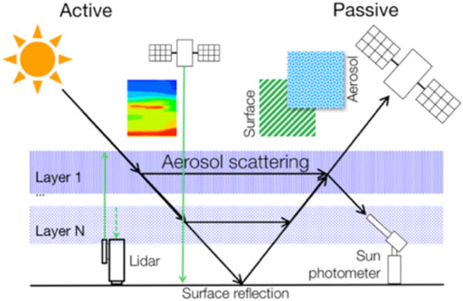
FIGURE 25. The illustration of combined ground-based and satellite observations that can be processed synergistically by GRASP.

It should be noted that synergetic processing of up- and down-looking observations from ground, airplane and satellite are useful not only for obtaining more accurate information about aerosol and surface reflectance properties but also for tuning different aspects of satellite retrieval algorithm. Indeed, in many cases satellite observations have significant limitation in the information content and additional assumptions are needed in order to reduce the number of the retrieved parameters. In these regards the joint synergic retrieval of aerosol and surface properties by simultaneous inversion of satellite and ground-based observations can be used for validating and tuning these assumptions. For example, Dubovik et al. (2011) has discussed the optimization of aerosol size distribution representation for observations with different information content. They suggested to use simplified aerosol model for POLDER like satellite retrieval with the size distribution approximated by 5 log-normal bins with fixed median sizes and standard deviations. Moreover, as discussed above even more constrained aerosol model was used for processing POLDER data, where aerosol was represented as external mixture (Eq 3.10‐3.11) of several aerosol components with fixed particles sizes, refractive indices and shapes and only the concentration of the components to be retrieved (see Chen et al., 2020; Lopatin et al., 2021). The verification of the validity of the assumptions taken can be checked using joint processing of satellite and ground-based observations. For example, 5 bins size distribution model and a mixture of aerosol components were applied for processing Sentinel-S5P observations. Figure 26 shows the results of joint inversion of collocated Sentinel-S5P and AERONET observations using 3 different models: 1) AERONET model with size distribution modeled using 22 triangle size bins, 2) model using 5 log-normal bins and 3) models representing aerosol by a mixture of predefined components. The joint retrievals showed that all three approaches allow rather accurate fitting of both AERONET and Sentinel-S5P with the best fit for the most detailed model and slightly degrading for the second and the third approaches. Moreover, the joint Sentinel-S5P and AERONET processing did not reveal neither evident limitations in fitting of the observations nor in agreement of the retrievals with available aerosol or surface. Figure 26 demonstrates that all three approaches can rather adequately reproduce all aerosol properties that agree with standard AERONET aerosol results including total AOD, and more detailed properties such as AE (Angstrom Exponent) and SSA.

FIGURE 26

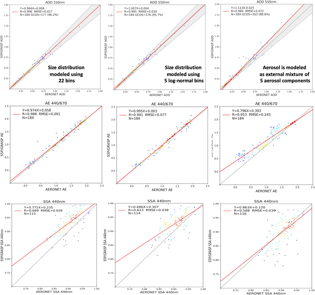
FIGURE 26. The correlations of AOD obtained from combined S5P + AERONET observations using aerosol models of different complexity with AERONET data. Upper panel: the correlation of obtained from combined S5P + AERONET with AERONET AOD measurements; The middle and lower panels: the correlations of Angstrom Exponent (AE) and SSA obtained from combined S5P + AERONET observations using aerosol models of different complexity with AERONET only operational results.

Finally, it should be emphasized that provided above examples of joint retrievals are only selected set of the most mature applications chosen to illustrate the broad possibilities in realizing synergetic processing of diverse remote sensing and in situ observations. The fact is that all data that currently can be processed by GRASP algorithm as those shown in diagram in Figure 21 can, in principle, be processed jointly in diverse combinations provided the observations were coordinated, i.e., taken in nearby location and in sufficiently close (for chosen application) moments of time. In future, the applicability of GRASP is expected to be further expanded.

5 Conclusion

The potential of utilizing Multi-term (Least Square Method) LSM approach for designing and improving retrieval algorithms in remote sensing has been discussed and illustrated in application. Both fundamental methodology of the approach and practical realizations were reviewed and discussed. The Multi-term LSM concept provides clear and efficient way of applying multiple a priori constraints that is not evident in the frame of Method Maximum Likelihood (MML) and LSM formulations. Indeed, the approach allows simultaneous application of diverse a priori constraints in the same retrieval and opens many potentially useful applications. For example, the AERONET retrieval of aerosol from ground-based observations by Dubovik and King (2000) used Multi-term LSM to apply several different a priori constraints simultaneously on several retrieved characteristics. As a result, AERONET retrieval uses a set of different smoothness a priori constraints allowing elimination of sharp variability in both retrieved aerosol size distributions and in spectral dependencies of real and imaginary part of refractive indices. Recently, Dubovik et al. (2011) and Dubovik et al. (2014) have designed algorithm called GRASP (Generalized Retrieval of Aerosol and Surface Properties) with an objective of more profound exploration of the Multi-term LSM approach in diverse remote sensing retrieval.

The following key methodological aspects of numerical Multi-term LSM inversion realized in GRASP were reviewed and discussed in the paper:

• It was outlined that the Multi-term LSM approach is fully based on MML and LSM developments and, therefore, the designed retrievals holds asymptotic optimality of the retrieved parameters, in sense of their error variances asymptotic approaching to the fundamental minimum accuracy boundaries related with Fisher information definition.

• It was shown that Multi-term LSM has the same base with Bayesian and Optimum Estimation (OE) (Rodgers 2000) approaches and can be considered as fundamentally equivalent methodology. At the same time, while Bayesian and OE methodologies rely on explicit representation of a priori constraints via a priori estimates of the state vector with known covariance matrix, Multi-term LSM in a contrast allows more flexible parameterization of a priori constraints, therefore providing more freedom in designing practical constrained inversion procedures.

• A possibility of including a priori knowledge about non-negativity of measurements or retrieved parameters was discussed and the statistical optimization of the inversion in the logarithmic space was recommended for positively defined values.

• Several details of realizing statistically optimized inversion for non-linear forward models were discussed and it was outlined that Levenberg-Marquardt non-linear inversion scheme can be optimized using Multi-term LSM optimization by considering linearization at each iteration as errors and as part of measurement uncertainties.

• An issue of possible domination in the retrieval by a rather similar and therefore possibly redundant observations was considered. For minimizing the possible negative effect of such domination, an assumption was adapted that the variance of error per measurement in data set increases proportionally to the total number of measurements in each data set. Such assumption is expected to reflect the general tendency of increasing overall uncertainty of a single observation related with an increase of the efforts in controlling more complex observation sets (with larger number of observation points).

• Multi-term LSM approach is aimed for the use of multiple a priori constraints assuming that different a priori assumptions come from the real knowledge and therefore consistent. The consistency of multiple a priori constraints can be verified based on the comparison of achieved value (“goodness of the fits”) of minimized quadratic term corresponding to each a priori constraint with the value expected based on the used assumptions.

• The estimations of the retrieval errors obtained in frame of Multi-term LSM approach allows for evaluating the contribution of measurement and a priori uncertainties on the retrieval accuracy. The strategy for accounting for the contribution of possible biases in the initial data or forward model is also discussed.

The GRASP algorithm is a practical retrieval tool realized as an open source software (https://www.grasp-open.com/). This paper provided detailed description of GRASP structure, discussed the algorithm evolution and overviewed the key technical details and its main applications. GRASP has two main independent modules. The first, numerical inversion, includes mathematical operations not related to the particular physical nature of the inverted data (in this case, remote sensing observations). The second, the forward model, is developed to simulate diverse atmospheric remote sensing observations, laboratory and in situ observations of light scattering and absorption. The forward model unit of GRASP is designed to simulate the interaction of electromagnetic radiation with atmospheric particles such as aerosol and clouds. The forward model of GRASP also accounts for gaseous absorption and for multiple interactions of light scattered by atmosphere and reflected by underlying surface using rigorous radiative transfer calculation in approximation of plane-parallel atmosphere. It allows the simulation of observations by diverse satellites, ground-based and airborne radiometers, spectrometers and lidars, in situ polar- and integrating-nephelometers, etc.

he independence of numerical inversion modules allows successful utilization of features realized in numerical inversion in many practical applications. Moreover, the coordinated observations of different type can be inverted simultaneously. This opens possibilities of exploring diverse synergetic approaches. The possibilities of simultaneous inversion of diverse combinations of multi-instrument observations were discussed in the paper. For example, one of the most popular GRASP synergetic retrieval is simultaneous inversion of passive radiometric and active lidar observation acquired from ground, satellite or airplane.

GRASP suggests using two rather distinct types of a priori constraints. The a priori constraints for strictly coincident and collocated observations are united in the group of “single-pixel” constraints. These constraints include direct a priori estimates of unknowns and smoothness constraints that can be applied for a group of retrieved parameters representing continuous functions, such as particle size or shape distributions, vertical profiles, spectrally dependent index of refraction or parameters of surface reflectance, etc. From the mathematic point of view, the smoothness constraints are applied by using a priori estimates of the first, second or third order derivatives of the retrieved function. The second group includes a priori constraints for coordinated but not fully coincident or/and not fully collocated observations are called “multi-pixel” constraints. For example, if a large group of satellite observations (“pixels” of the image) is inverted simultaneously, the concept of multi-pixel constraints allows for constraining the retrieval results by using known a priori limitation of variability of the retrieved parameters in time and or space. For example, in many satellite retrievals realized by GRASP the known natural tendencies are used: variability of land surface reflectance is quite limited in time while aerosol properties have an evident horizontal continuity. The strength of all a priori constraints can be different for each of the retrieved parameters. It should be noted that a concept of multi-pixel retrieval opens extra possibilities for synergetic processing of non-coincident or/and non-collocated observations. For example, this concept was used for joint processing of day- and night-time radiometric, photometric and lidar observations. More complex constraints that currently are not included neither in single- nor in multi-pixel constraints could also be realized in GRASP with some extra efforts if the need is identified or by request.

GRASP has been successfully adapted for a number of practical applications demonstrated in the paper. For example, the algorithm was used to generate an advanced aerosol product from series of multi-angular POLDER polarimeters. POLDER/GRASP retrieval provided the values of spectral AOD and other detailed aerosol parameters including Angstrom parameter, spectral AOD for fine and coarse aerosol modes, as well as spectral AAOD and SSA. The spectral values of land and ocean surface BRDF and BPDF were retrieved simultaneously with aerosol. GRASP is used in preparation of operational aerosol algorithms for the future 3MI/EPS-SG and CO2M polarimetric missions. It was shown to provide solid aerosol retrieval for multi-angular MISR observations. In addition, aerosol AOD product from single-view MERIS/Envisat radiometer was generated using GRASP. Finally, the algorithm is also being adapted for AOD and surface reflectance retrievals from observations by more recent and future satellites including OLCI/Sentinel-3, Sentinel-4, TROPOMI/Sentinel- 5P, HIMAWARI, MISR, SGLI/GICOM-C, etc.

GRASP has been used quite extensively for retrieving aerosol from ground-based and in situ observations. For example, the algorithm was used for polar- and integrating-nephelometric measurements of angular aerosol scattering, total absorption and scattering for retrieving aerosol size, shape and information about the composition. One of the most popular GRASP applications, known as GRASP/GARRLiC, is retrieval of both columnar and vertical aerosol properties from a combination of collocated passive radiometric and active lidar observations. Such GRASP/GARRLiC approach is adapted by ACTRIS pan-European research infrastructure as a part of operational data processing. Recently similar synergetic processing was extended in the frame of GRASP for joint inversion of active and passive satellite observations. As a result, such GRASP configuration was incorporated in a new aerosol retrieval testbed developed for exploring the capabilities of synergistic passive and active remote sensing in frame of NASA ACPP initiative.

Furthermore, in the frame of GRASP a new approach has been developed for retrieval of aerosol chemical components directly from satellite and ground-based measurements. The observed aerosols are assumed to be mixtures of hydrated soluble particles embedded with black carbon, brown carbon, iron oxide, and dust or organic carbon insoluble inclusions and the volume fractions of these components are derived along with aerosol size and shape information. This component approach was successfully applied to POLDER satellite and AERONET observations.

The paper also mentions other diverse less mature GRASP applications that are under development or expected to be fully realized in the near future. For example, GRASP is being adapted for profound use of hyper spectral measurements with an objective of using measurements of atmospheric absorption for advanced retrieval of information about both atmospheric aerosol and gases. In these regards, GRASP is being expanded for retrieval of also atmospheric gases in addition to aerosol and surface and, to reflect this development GRASP should be renamed as Generalized Retrieval of Atmosphere and Surface Properties.

Data Availability Statement

The original contributions presented in the study are included in the article/Supplementary Material, further inquiries can be directed to the corresponding author.

Author Contributions

OD - inversion theory, methodology, concept of GRASP, DF - GRASP applications, figures, PL - advancements of forward model, AL - methodology for active observations in GRASP, TL - software implementation of GRASP, ID - MML asymptotical properties, FX-inversion methodology, FD - implementation of POLDER applications, CC - diverse data analysis, BT - implementation of GRASP-AOD module, YD - scientific analysis, radiative forcing, LL - development of GRASP/Component approach, MH-G - hyperspectral and TIR applications, MH - error estimations, YK - manuscript editing and polishing, CM - data analysis, GS - application of GRASP to nephelometrers editing, RE - application of GRASP to nephelometrs and for ACCP studies, AP - application of GRASP to HARP, ZL - discussion of GRASP concept and applications, JFr and RP - adaption to hyperspectral data, JC - using GRASP for ACCP lidar studies, AK, AC, and MA - application to real hyperspectral data, Aspetsberger, DM, LB, AH, VL, CH, and CF - software implementations.

Conflict of Interest

Authors DF, PL, AL, ID, CC, MH-G, YK, and CM were employed by the company GRASP-SAS. Authors AK and AC were employed by the company LuftBlick OG. Authors MA, DM, LB, AH, VL, CH, and CF were employed by the company Cloudflight GmbH. OD supported GRASP SAS with scientific consulting and held the actions of the company under “concours scientifique” convention of CNRS.

The remaining authors declare that the research was conducted in the absence of any commercial or financial relationships that could be construed as a potential conflict of interest.

Publisher’s Note

All claims expressed in this article are solely those of the authors and do not necessarily represent those of their affiliated organizations, or those of the publisher, the editors and the reviewers. Any product that may be evaluated in this article, or claim that may be made by its manufacturer, is not guaranteed or endorsed by the publisher.

Acknowledgments

The authors are grateful for the continuing support of GRASP developments: - from ESA in frame of multiple projects including IDEAS, CAWA, DIVA, QA4EO, aerosol retrieval developments for Sentinel -4, 5P and -7, etc., - from EUMETSAT in frame of multiple projects OLCI/Sentinel-3, 3MI/EPS-SG and MAP/S-7, - from CNES for POLDER-3/PARASOL, 3MI/EPS-SG, ACCP/EECLAT, etc., - from European Commission in frame of GRASP-ACE grant. The authors acknowledge the support from the Chemical and Physical Properties of the Atmosphere Project funded by the French National Research Agency through the Programme d’Investissement d’Avenir under contract ANR-11-LABX-0 0 05-01, the Regional Council “Hauts-de-France”, and the “European Funds for Regional Economic Development”, from Research grant (no. URF/1/2180-01-01 ) “Combined Radiative and Air Quality Effects of Anthropogenic”. Also, the authors acknowledge the support from the European Metrology Program for Innovation and Research (EMPIR) within the joint research project EMPIR 19ENV04 MAPP “Metrology for aerosol optical properties”. The EMPIR is jointly funded by the EMPIR participating countries within EURAMET and the European Union. OD expresses personal thanks to B. Bojkov, formerly from ESA and currently from EUMETSAT, for his continuing support and encouragement of theoretical developments of Multi-term LSM inversion methodology and its applications in atmospheric remote sensing. Also, OD thanks G. Stenchikov for fruitful discussions and collaborations on optimizing GRASP application for ground-based and air-borne observations.

References

Agresti, A., and Hitchcock, D. B. (2005). Bayesian Inference for Categorical Data Analysis. Jiss 14 (14), 297–330. doi:10.1007/s10260-005-0121-y

CrossRef Full Text | Google Scholar

Aspetsberger, M., Amberger, S., Cobarzan, P., Bindreiter, L., Hangler, A., Lanzinger, V., et al. (2019). The GRASP Cloud – Application and Demonstration, 2-nd International Workshop. Lille, France: APOLO-2, 4-7.

Google Scholar

Brogniez, G., Pietras, C., Legrand, M., Dubuisson, P., and Haeffelin, M. (2003). A high-accuracy multiwavelength radiometer for in situ measurements in the thermal infrared. Part II: Behavior in field experiments. J. Atmos. Ocean. Tech., 122, 1023–1033.

CrossRef Full Text | Google Scholar

Benavent-Oltra, J. A., Casquero-Vera, J. A., Román, R., Lyamani, H., Pérez-Ramírez, D., Granados-Muñoz, M. J., et al. (2021). Overview of SLOPE I and II Campaigns: Aerosol Properties Retrieved with Lidar and Sun-Sky Photometer Measurements. Atmos. Chem. Phys. Discuss. 21, 9269–9287. doi:10.5194/acp-2021-66

CrossRef Full Text | Google Scholar

Benavent-Oltra, J. A., Román, R., Casquero-Vera, J. A., Pérez-Ramírez, D., Lyamani, H., Ortiz-Amezcua, P., et al. (2019). Different Strategies to Retrieve Aerosol Properties at Night-Time with the GRASP Algorithm. Atmos. Chem. Phys. 19, 14149–14171. doi:10.5194/acp-19-14149-2019

CrossRef Full Text | Google Scholar

Benavent-Oltra, J. A., Román, R., Granados-Muñoz, M. J., Pérez-Ramírez, D., Ortiz-Amezcua, P., Denjean, C., et al. (2017). Comparative Assessment of GRASP Algorithm for a Dust Event over Granada (Spain) during ChArMEx-ADRIMED 2013 Campaign. Atmos. Meas. Tech. 10, 4439–4457. doi:10.5194/amt-10-4439-2017

CrossRef Full Text | Google Scholar

Blumstein, D., Chalon, G., Carlier, T., Buil, C., Hebert, P., Maciaszek, T., et al. (2004). “IASI Instrument: Technical Overview and Measured Performances,” in Infrared Spaceborne Remote Sensing XII, Editor M. Strojnik, (International Society for Optics and Photonics), 5543, 196–207. doi:10.1117/12.560907

CrossRef Full Text | Google Scholar

Bovchaliuk, A., Milinevsky, G., Danylevsky, V., Goloub, P., Dubovik, O., Holdak, A., et al. (2013). Variability of Aerosol Properties over Eastern Europe Observed from Ground and Satellites in the Period from 2003 to 2011. Atmos. Chem. Phys. 13, 6587–6602. doi:10.5194/acp-13-6587-2013

CrossRef Full Text | Google Scholar

Bovchaliuk, V., Goloub, P., Podvin, T., Veselovskii, I., Tanre, D., Chaikovsky, A., et al. (2016). Comparison of Aerosol Properties Retrieved Using GARRLiC, LIRIC, and Raman Algorithms Applied to Multi-Wavelength LIDAR and Sun/sky-Photometer Data. Atmos. Meas. Tech.Atmos. Meas. Tech. 9, 3391–3405. doi:10.5194/amt-9-3391-2016

CrossRef Full Text | Google Scholar

Chahine, M. T. (1968). Determination of the Temperature Profile in an Atmosphere from its Outgoing Radiance*. J. Opt. Soc. Am. 58, 1634–1637. doi:10.1364/josa.58.001634

CrossRef Full Text | Google Scholar

Chen, C., Dubovik, O., Fuertes, D., Litvinov, P., Lapyonok, T., Lopatin, A., et al. (2020). Validation of GRASP Algorithm Product from POLDER/PARASOL Data and Assessment of Multi-Angular Polarimetry Potential for Aerosol Monitoring. Earth Syst. Sci. Data 12, 3573–3620. doi:10.5194/essd-12-3573-20202020

CrossRef Full Text | Google Scholar

Chen, C., Dubovik, O., Henze, D. K., Chin, M., Lapyonok, T., Schuster, G. L., et al. (2019). Constraining Global Aerosol Emissions Using POLDER/PARASOL Satellite Remote Sensing Observations. Atmos. Chem. Phys. 19, 14585–14606. doi:10.5194/acp-19-14585-2019

CrossRef Full Text | Google Scholar

Chen, C., Dubovik, O., Henze, D. K., Lapyonak, T., Chin, M., Ducos, F., et al. (2018). Retrieval of Desert Dust and Carbonaceous Aerosol Emissions over Africa from POLDER/PARASOL Products Generated by the GRASP Algorithm. Atmos. Chem. Phys. 18, 12551–12580. doi:10.5194/acp-18-12551-2018

CrossRef Full Text | Google Scholar

Cox, C., and Munk, W. (1954). Measurement of the Roughness of the Sea Surface from Photographs of the Sun's Glitter. J. Opt. Soc. Am. 44, 838–850. doi:10.1364/josa.44.000838

CrossRef Full Text | Google Scholar

Cuesta, J. (2021). Type Discriminated Aerosol Concentration Profile Derived from the ACCP Lidar Spaceborne Multispectral Measurements. CALIPSO Version 5 Aerosol Lidar Ratio Workshop, 9–11.

Google Scholar

Derimian, Y., Dubovik, O., Huang, X., Lapyonok, T., Litvinov, P., Kostinski, A. B., et al. (2016). Comprehensive Tool for Calculation of Radiative Fluxes: Illustration of Shortwave Aerosol Radiative Effect Sensitivities to the Details in Aerosol and Underlying Surface Characteristics. Atmos. Chem. Phys. 16, 5763–5780. doi:10.5194/acp-16-5763-2016

CrossRef Full Text | Google Scholar

Deuzé, J. L., Bréon, F. M., Devaux, C., Goloub, P., Herman, M., Lafrance, B., et al. (2001). Remote Sensing of Aerosols over Land Surfaces from POLDER-ADEOS-1 Polarized Measurements. J. Geophys. Res. 106, 4913–4926. doi:10.1029/2000JD900364

CrossRef Full Text | Google Scholar

Deuzé, J. L., Herman, M., Goloub, P., Tanré, D., and Marchand, A. (1999). Characterization of Aerosols over Ocean from POLDER/ADEOS-1. Geophys. Res. Lett. 26, 1421–1424. doi:10.1029/1999GL900168

CrossRef Full Text | Google Scholar

Dolgos, G., and Martins, J. V. (2014). Polarized Imaging Nephelometer for In Situ Airborne Measurements of Aerosol Light Scattering. Opt. Express 22, 21972–21990. doi:10.1364/OE.22.021972

PubMed Abstract | CrossRef Full Text | Google Scholar

Doppler, L., Preusker, R., Bennartz, R., and Fischer, J. (2014). K-Bin and K-IR: K-Distribution Methods without Correlation Approximation for Non-fixed Instrument Response Function and Extension to the thermal Infrared-Applications to Satellite Remote Sensing. J. Quantitative Spectrosc. Radiative Transfer 133, 382–395. doi:10.1016/j.jqsrt.2013.09.001

CrossRef Full Text | Google Scholar

Dubovik, O., Herman, M., Holdak, A., Lapyonok, T., Tanré, D., Deuzé, J. L., et al. (2011). Statistically Optimized Inversion Algorithm for Enhanced Retrieval of Aerosol Properties from Spectral Multi-Angle Polarimetric Satellite Observations. Atmos. Meas. Tech. 4, 975–1018. doi:10.5194/amt-4-975-2011

CrossRef Full Text | Google Scholar

Dubovik, O., Holben, B., Eck, T. F., Smirnov, A., Kaufman, Y. J., King, M. D., et al. (2002). Variability of Absorption and Optical Properties of Key Aerosol Types Observed in Worldwide Locations. J. Atmos. Sci. 59, 590–608. doi:10.1175/1520-0469(2002)059<0590:voaaop>2.0.co;2

CrossRef Full Text | Google Scholar

Dubovik, O., and King, M. D. (2000). A Flexible Inversion Algorithm for Retrieval of Aerosol Optical Proper-Ties from Sun and Sky Radiance Measurements. J. Geophys. Res. 105, 673–696. doi:10.1029/2000jd900282

CrossRef Full Text | Google Scholar

Dubovik, O., Lapyonok, T., Kaufman, Y. J., Chin, M., Ginoux, P., Kahn, R. A., et al. (2008). Retrieving Global Aerosol Sources from Satellites Using Inverse Modeling. Atmos. Chem. Phys. 8, 209–250. doi:10.5194/acp-8-209-2008

CrossRef Full Text | Google Scholar

Dubovik, O., Lapyonok, T., Litvinov, P., Herman, M., Fuertes, D., Ducos, F., et al. (2014). GRASP: A Versatile Algorithm for Characterizing the Atmosphere. SPIE: Newsroom. doi:10.1117/2.1201408.005558

CrossRef Full Text | Google Scholar

Dubovik, O., Li, Z., Mishchenko, M. I., Tanré, D., Karol, Y., Bojkov, B., et al. (2019). Polarimetric Remote Sensing of Atmospheric Aerosols: Instruments, Methodologies, Results, and Perspectives. J. Quantitative Spectrosc. Radiative Transfer 224, 474–511. doi:10.1016/j.jqsrt.2018.11.024

CrossRef Full Text | Google Scholar

Dubovik, O. (2004). “Optimization of Numerical Inversion in Photopolarimetric Remote Sensing,” in Photopolarimetry in Remote Sensing. Editors G. Videen, Y. Yatskiv, and M. Mishchenko (Dordrecht, Netherlands: Kluwer Academic Publishers), 65–106.

Google Scholar

Dubovik, O., Schuster, G. L., Xu, F., Hu, Y., Bösch, H., Landgraf, J., et al. (2021). Grand Challenges in Satellite Remote Sensing. Front. Remote Sens. 2, 619818. doi:10.3389/frsen.2021.619818

CrossRef Full Text | Google Scholar

Dubovik, O., Sinyuk, A., Lapyonok, T., Holben, B. N., Mishchenko, M., Yang, P., et al. (2006). Application of Spheroid Models to Account for Aerosol Particle Nonsphericity in Remote Sensing of Desert Dust. J. Geophys. Res. 111, D11208. doi:10.1029/2005JD006619d

CrossRef Full Text | Google Scholar

Dubovik, O., Smirnov, A., Holben, B. N., King, M. D., Kaufman, Y. J., Eck, T. F., et al. (2000). Accuracy Assessments of Aerosol Optical Properties Retrieved from Aerosol Robotic Network (AERONET) Sun and Sky Radiance Measurements. J. Geophys. Res. 105, 9791–9806. doi:10.1029/2000jd900040

CrossRef Full Text | Google Scholar

Dubovik, O. V., Lapyonok, T. V., and Oshchepkov, S. L. (1995). Improved Technique for Data Inversion: Optical Sizing of Multicomponent Aerosols. Appl. Opt. 34, 8422–8436. doi:10.1364/ao.34.008422

PubMed Abstract | CrossRef Full Text | Google Scholar

Edie, W. T., Dryard, D., James, F. E., Roos, M., and Sadoulet, B. (1971). Statistical Methods in Experimental Physics. New York: North-Holland, 155.

Google Scholar

Elguindi, N., Granier, C., Stavrakou, T., Darras, S., Bauwens, M., Cao, H., et al. (2020). Intercomparison of Magnitudes and Trends in Anthropogenic Surface Emissions from Bottom‐Up Inventories, Top‐Down Estimates, and Emission Scenarios. Earth's Future 8, e2020EF001520. doi:10.1029/2020EF001520

CrossRef Full Text | Google Scholar

Espinosa, W. R., Castellanos, P., Sayer, A., Colarco, P., Kemppien, O., Nowottnick, E., et al. (2019b). “An Exploration of Joint LIDAR and Multiangle Polarimeter Aerosol Retrieval Capabilities Using the GRASP Algorithm and OSSE Data Derived from the GEOS Model,” in The 2nd Conference on Advancement of POLarimetric Observations (France: Lille), 04–09.

Google Scholar

Espinosa, W. R., Martins, J. V., Remer, L. A., Dubovik, O., Lapyonok, T., Fuertes, D., et al. (2019a). Retrievals of Aerosol Size Distribution, Spherical Fraction, and Complex Refractive Index from Airborne In Situ Angular Light Scattering and Absorption Measurements. J. Geophys. Res. Atmos. 124, 7997–8024. doi:10.1029/2018JD030009

CrossRef Full Text | Google Scholar

Espinosa, W. R., Remer, L. A., Dubovik, O., Ziemba, L., Beyersdorf, A., Orozco, D., et al. (2017). Retrievals of Aerosol Optical and Microphysical Properties from Imaging Polar Nephelometer Scattering Measurements. Atmos. Meas. Tech. 10, 811–824. doi:10.5194/amt-10-811-2017

PubMed Abstract | CrossRef Full Text | Google Scholar

Fisher, R. A. (1956). Statistical Methods and Scientific Inference. New York: Hafner Publishing Co.

Google Scholar

Fougnie, B., Marbach, T., Lacan, A., Lang, R., Schlüssel, P., Poli, G., et al. (2019). The Multi-Viewing Multi-Channel Multi-Polarisation Imager – Overview of the 3MI Polarimetric mission for Aerosol and Cloud Characterization. J. Quant Spectrosc. Radiat. Transfer 219, 23–32.

Google Scholar

Fourgeaut, C., and Fuchs, A. (1967). Statisque. Paris: Dunod, 326.

Google Scholar

Freudenthaler, V., Esselborn, M., Wiegner, M., Heese, B., Tesche, M., Ansmann, A., et al. (2009). Depolarization Ratio Profiling at Several Wavelengths in Pure Saharan Dust during SAMUM 2006. Tellus B: Chem. Phys. Meteorology 61, 165–179. doi:10.1111/j.1600-0889.2008.00396.x

CrossRef Full Text | Google Scholar

Frouin, R. J., Franz, B. A., Ibrahim, A., Knobelspiesse, K., Ahmad, Z., Cairns, B., et al. (2019). Atmospheric Correction of Satellite Ocean-Color Imagery during the PACE Era. Front. Earth Sci. 7, 145. doi:10.3389/feart.2019.00145

PubMed Abstract | CrossRef Full Text | Google Scholar

Fu, G., Hasekamp, O., Rietjens, J., Smit, M., Di Noia, A., Cairns, B., et al. (2020). Aerosol Retrievals from Different Polarimeters during the ACEPOL Campaign Using a Common Retrieval Algorithm. Atmos. Meas. Tech. 13, 553–573. doi:10.5194/amt-13-553-2020

CrossRef Full Text | Google Scholar

Fuertes, D., Dubovik, O., Hangler, A., Lytvynov, P., Lopatin, A., Aspetsberger, M., et al. (2020). Retrieval of Aerosol Prop-Erties from MISR Observations Using GRASP Algorithm: Methodology, Products and Validation. AGU Fall Meeting, 9–17.

Google Scholar

Fuertes, D., Nicolae, D., Dubovik, O., Torres, B., Goloub, P., Lopatin, A., et al. (2019). DIVA: Demonstration of an Integrated Approach for the Validation and Exploitation of Atmospheric Missions. San Francisco, CA, USA: AGU Fall Meeting, 9–13.

Google Scholar

Garnier, A., Pelon, J., Dubuisson, P., Faivre, M., Chomette, O., Pascal, N., et al. (2012). Retrieval of Cloud Properties Using CALIPSO Imaging Infrared Radiometer. Part I: Effective Emissivity and Optical Depth. J. Appl. Meteorology Climatology 51 (7), 1407–1425. doi:10.1175/jamc-d-11-0220.1

CrossRef Full Text | Google Scholar

Gatebe, C. K., Dubovik, O., King, M. D., and Sinyuk, A. (2010). Simultaneous Retrieval of Aerosol and Surface Optical Properties from Combined Airborne- and Ground-Based Direct and Diffuse Radiometric Measurements. Atmos. Chem. Phys. 10, 2777–2794. doi:10.5194/acp-10-2777-2010

CrossRef Full Text | Google Scholar

Govaerts, Y. M., Wagner, S., Lattanzio, A., and Watts, P. (2010). Joint Retrieval of Surface Reflectance and Aerosol Optical Depth from MSG/SEVIRI Observations with an Optimal Estimation Approach: 1. Theory. J. Geophys. Res. 115, D02203. doi:10.1029/2009JD011779

CrossRef Full Text | Google Scholar

Hair, J. W., Hostetler, C. A., Cook, A. L., Harper, D. B., Ferrare, R. A., Mack, T. L., et al. (2008). Airborne High Spectral Resolution Lidar for Profiling Aerosol Optical Properties. Appl. Opt. 47, 6734–6753. doi:10.1364/ao.47.006734

PubMed Abstract | CrossRef Full Text | Google Scholar

Hansen, P. C. (1992). Numerical Tools for Analysis and Solution of Fredholm Integral Equations of the First Kind. Inverse Probl. 8, 849–872. doi:10.1088/0266-5611/8/6/005

CrossRef Full Text | Google Scholar

Hasekamp, O. P., Fu, G., Rusli, S. P., Wu, L., Di Noia, A., Brugh, J. a. d., et al. (2019). Aerosol Measurements by SPEXone on the NASA PACE mission: Expected Retrieval Capabilities. J. Quantitative Spectrosc. Radiative Transfer 227, 170–184. doi:10.1016/j.jqsrt.2019.02.006

CrossRef Full Text | Google Scholar

Hasekamp, O. P., and Landgraf, J. (2005). Linearization of Vector Radiative Transfer with Respect to Aerosol Properties and its Use in Satellite Remote Sensing. J. Geophys. Res. 110, D04203. doi:10.1029/2004JD005260

CrossRef Full Text | Google Scholar

Hasekamp, O. P., and Landgraf, J. (2007). Retrieval of Aerosol Properties over Land Surfaces: Capabilities of Multiple-Viewing-Angle Intensity and Polarization Measurements. Appl. Opt. 46, 3332–3344. doi:10.1364/AO.46.003332

PubMed Abstract | CrossRef Full Text | Google Scholar

Herman, J., Cede, A., Spinei, E., Mount, G., Tzortziou, M., and Abuhassan, N. (2009). NO2column Amounts from Ground-Based Pandora and MFDOAS Spectrometers Using the Direct-Sun DOAS Technique: Intercomparisons and Application to OMI Validation. J. Geophys. Res. 114, D13307. doi:10.1029/2009JD011848

CrossRef Full Text | Google Scholar

Herman, J., Evans, R., Cede, A., Abuhassan, N., Petropavlovskikh, I., and McConville, G. (2015). Comparison of Ozone Retrievals from the Pandora Spectrometer System and Dobson Spectrophotometer in Boulder, Colorado. Atmos. Meas. Tech. 8, 3407–3418. doi:10.5194/amt-8-3407-2015

CrossRef Full Text | Google Scholar

Herman, M., Deuzé, J. L., Marchand, A., Roger, B., and Lallart, P. (2005). Aerosol Remote Sensing from POLDER/ADEOS over the Ocean: Improved Retrieval Using a Nonspherical Particle Model. J. Geophys. Res. 110, D10S02. doi:10.1029/2004JD004798

CrossRef Full Text | Google Scholar

Herrera, M., Dubovik, O., Torres, B., Lapyonok, T., Litvinov, P., Chen, C., et al. (2020). Rigorous Estimates of the Retrieval Errors in Diverse Remote Sensing Applications provided by GRASP Algorithm. AGU Fall Meeting, 9–17.

Google Scholar

Herreras, M., Litvinov, P., Derimian, Y., Dubovik, O., Lapyonok, T., and Fuertes, D. (2020). Emission Inclusion in Successive Orders of Scattering Radiative Transfer Scheme. AGU Fall Meeting, 9–17.

Google Scholar

Herreras, M., Román, R., Cazorla, A., Toledano, C., Lyamani, H., Torres, B., et al. (2019). Evaluation of Retrieved Aerosol Extinction Profiles Using as Reference the Aerosol Optical Depth Differences between Various Heights. Atmos. Res. 230, 104625. doi:10.1016/j.atmosres.2019.104625

CrossRef Full Text | Google Scholar

Herreras-Giralda, M., Dubovik, O., Fuertes, D., Layponok, T., Litvinov, P., Derimian, Y., et al. (in preparation). Simultaneous Retrieval of Aerosol Properties and Gas Concentration with GRASP Algorithm.

Google Scholar

Holben, B. N., Eck, T. F., Slutsker, I., Tanré, D., Buis, J. P., Setzer, A., et al. (1998). AERONET-A Federated Instrument Network and Data Archive for Aerosol Characterization. Remote Sensing Environ. 66, 1–16. doi:10.1016/s0034-4257(98)00031-5

CrossRef Full Text | Google Scholar

Hu, Q., Goloub, P., Bravo-Aranda, J.-A., Popovici, I. E., Podvin, T., Haeffelin, M., et al. (2019). Long-range-transported Canadian Smoke Plumes in the Lower Stratosphere over Northern France. Atmos. Chem. Phys. 19, 1173–1193. doi:10.5194/acp-19-1173-2019

CrossRef Full Text | Google Scholar

Jones, S. H., King, M. D., and Ward, A. D. (2013). Determining the Unique Refractive index Properties of Solid Polystyrene Aerosol Using Broadband Mie Scattering from Optically Trapped Beads. Phys. Chem. Chem. Phys. 15, 20735–20741. doi:10.1039/c3cp53498g

PubMed Abstract | CrossRef Full Text | Google Scholar

Justice, C. O., Vermote, E., Townshend, J. R. G., Defries, R., Roy, D. P., Hall, D. K., et al. (1998). The Moderate Resolution Imaging Spectroradiometer (MODIS): Land Remote Sensing for Global Change Research. IEEE Trans. Geosci. Remote Sensing 36, 1228–1249. doi:10.1109/36.701075

CrossRef Full Text | Google Scholar

Kato, S., Ackerman, T. P., Mather, J. H., and Clothiaux, E. E. (1999). The K-Distribution Method and Correlated-K Approximation for a Shortwave Radiative Transfer Model. J. Quantitative Spectrosc. Radiative Transfer 62, 109–121. doi:10.1016/s0022-4073(98)00075-2

CrossRef Full Text | Google Scholar

King, M. D., Byrne, D. M., Herman, B. M., and Reagan, J. A. (1978). Aerosol size distributions obtained by inversion of spectral optical depth measurements. J. Atmos. Sci. 21, 2153–2167.

CrossRef Full Text | Google Scholar

King, M. D., and Dubovik, O. (2013). “Determination of Aerosol Optical Properties from Inverse Methods,” in Aerosol Remote Sensing. Editors J. Lenoble, L. Remer, and D. Tanré (Chischester, UK: Springer, Praxis Publishers), 101–136. doi:10.1007/978-3-642-17725-5_5

CrossRef Full Text | Google Scholar

Knobelspiesse, K., Cairns, B., Mishchenko, M., Chowdhary, J., Tsigaridis, K., van Diedenhoven, B., et al. (2012). Analysis of fine-mode Aerosol Retrieval Capabilities by Different Passive Remote Sensing Instrument Designs. Opt. Express 20, 21457–21484. doi:10.1364/OE.20.021457

PubMed Abstract | CrossRef Full Text | Google Scholar

Koepke, P. (1984). Effective Reflectance of Oceanic Whitecaps. Appl. Opt. 23, 1816. doi:10.1364/AO.23.001816

PubMed Abstract | CrossRef Full Text | Google Scholar

Kokhanovsky, A. A., and Breon, F.-M. (2012). Validation of an Analytical Snow BRDF Model Using PARASOL Multi-Angular and Multispectral Observations. IEEE Geosci. Remote Sensing Lett. 9 (5), 928–932. doi:10.1109/LGRS.2012.2185775

CrossRef Full Text | Google Scholar

Kokhanovsky, A. A., Davis, A. B., Cairns, B., Dubovik, O., Hasekamp, O. P., Sano, I., et al. (2015). Space-based Remote Sensing of Atmospheric Aerosols: The Multi-Angle Spectro-Polarimetric Frontier. Earth-Science Rev. 145, 85–116. doi:10.1016/j.earscirev.2015.01.012

CrossRef Full Text | Google Scholar

Kokhanovsky, A. A., Deuzé, J. L., Diner, D. J., Dubovik, O., Ducos, F., Emde, C., et al. (2010). The Inter-comparison of Major Satellite Aerosol Retrieval Algorithms Using Simulated Intensity and Polarization Characteristics of Reflected Light. Atmos. Meas. Tech. 3, 909–932. doi:10.5194/amt-3-909-2010

CrossRef Full Text | Google Scholar

Kokhanovsky, A. A., and Zege, E. P. (2004). Scattering Optics of Snow. Appl. Opt. 43 (7), 1589–1602. doi:10.1364/AO.43.001589

PubMed Abstract | CrossRef Full Text | Google Scholar

Kolmagorov, A. N. (1987). Theory of Information and Theory of Algorithms. Moskow: Nauka.

Google Scholar

Konsta, D., Tsekeri, A., Solomos, S., Siomos, N., Gialitaki, A., Tetoni, E., et al. (2021). The Potential of GRASP/GARRLiC Retrievals for Dust Aerosol Model Evaluation: Case Study during the PreTECT Campaign. Remote Sensing 13, 873. doi:10.3390/rs13050873

CrossRef Full Text | Google Scholar

Legrand, M., Pietras, C., Brogniez, G., Haeffelin, M., Abuhassan, N. K., and Sicard, M. (2000). A high-accuracy multiwavelength radiometer for in situ measurements in the thermal infrared. Part I: Characterization of the instrument J. Atmos. Ocean. Tech. 17 (9), 1203–1214.

CrossRef Full Text | Google Scholar

Lenoble, J., Herman, M., Deuzé, J. L., Lafrance, B., Santer, R., and Tanré, D. (2007). A Successive Order of Scattering Code for Solving the Vector Equation of Transfer in the Earth's Atmosphere with Aerosols. J. Quantitative Spectrosc. Radiative Transfer 107 (3), 479–507. doi:10.1016/j.jqsrt.2007.03.010

CrossRef Full Text | Google Scholar

Li, L., Che, H., Derimian, Y., Dubovik, O., Luan, Q., Li, Q., et al. (2020b). Climatology of fine and Coarse Mode Aerosol Optical Thickness over East and South Asia Derived from POLDER/PARASOL Satellite. J. Geophys. Res. Atmos. 125, e2020JD032665. doi:10.1029/2020JD032665

CrossRef Full Text | Google Scholar

Li, L., Che, H., Derimian, Y., Dubovik, O., Schuster, G. L., Chen, C., et al. (2020a). Retrievals of fine Mode Light-Absorbing Carbonaceous Aerosols from POLDER/PARASOL Observations over East and South Asia. Remote Sensing Environ. 247, 111913. doi:10.1016/j.rse.2020.111913

CrossRef Full Text | Google Scholar

Li, L., Dubovik, O., Derimian, Y., Schuster, G. L., Lapyonok, T., Litvinov, P., et al. (2019). Retrieval of Aerosol Components Directly from Satellite and Ground-Based Measurements. Atmos. Chem. Phys. 19, 13409–13443. doi:10.5194/acp-19-13409-2019

CrossRef Full Text | Google Scholar

Li, X., and Strahler, A. H. (1992). Geometric-optical Bidirectional Reflectance Modeling of the Discrete crown Vegetation Canopy: Effect of crown Shape and Mutual Shadowing. IEEE Trans. Geosci. Remote Sensing 30, 276–292. doi:10.1109/36.134078

CrossRef Full Text | Google Scholar

Linnik, U. V. (1962). Least Square Method and the Basic Theory of Observation Analysis. Moscow: Fizmatgiz, 350.

Google Scholar

Litvinov, P., Dubovik, O., Xuang, X., Lapyonok, T., Ducos, F., Lopatin, A., et al. (2018). “Advanced Surface/atmosphere Characterization with GRASP and Transition from Course to fine Spatial Resolution Retrieval,” in 2018 Workshop on Land Product Validation and Evolution (LPVE 2018) (Italy: ESA/ESRIN, Frascati), 27.

Google Scholar

Litvinov, P., Hasekamp, O., Cairns, B., and Mishchenko, M. (2010). Reflection Models for Soil and Vegetation Surfaces from Multiple-Viewing Angle Photopolarimetric Measurements. J. Quantitative Spectrosc. Radiative Transfer 111, 529–539. doi:10.1016/j.jqsrt.2009.11.001

CrossRef Full Text | Google Scholar

Litvinov, P., Hasekamp, O., Cairns, B., and Mishchenko, M. (2011b). “Semi-empirical BRDF and BPDF Models Applied to the Problem of Aerosol Retrievals over Land: Testing an Airborne Data and Implications for Modeling of Top-Of-Atmosphere Measurements,” in Book: Polarimetric Detection, Characterization, and Remote Sensing (Springer).

Google Scholar

Litvinov, P., Hasekamp, O., and Cairns, B. (2011a). Models for Surface Reflection of Radiance and Polarized Radiance: Comparison with Airborne Multi-Angle Photopolarimetric Measurements and Implications for Modeling Top-Of-Atmosphere Measurements. Remote Sensing Environ. 115, 781–792. doi:10.1016/j.rse.2010.11.005

CrossRef Full Text | Google Scholar

Litvinov, P., Hasekamp, O., Dubovik, O., and Cairns, B. (2012). Model for Land Surface Reflectance Treatment: Physical Derivation, Application for Bare Soil and Evaluation on Airborne and Satellite Measurements. J. Quantitative Spectrosc. Radiative Transfer 113, 2023–2039. doi:10.1016/j.jqsrt.2012.06.027

CrossRef Full Text | Google Scholar

Lopatin, A., Dubovik, O., Chaikovsky, A., Goloub, Ph., Lapyonok, T., Tanré, D., et al. (2013). “Enhancement of Aerosol Characterization Using Synergy of Lidar and Sun – Photometer Coincident Observations: the GARRLiC Algorithm”. Atmos. Meas. Tech. 13, 6587–6602. doi:10.5194/acp-13-6587-2013

CrossRef Full Text | Google Scholar

Lopatin, A., Dubovik, O., Fuertes, D., Stenchikov, G., Lapyonok, T., Veselovskii, I., et al. (2021). Synergy Processing of Diverse Ground-Based Remote Sensing and In Situ Data Using the GRASP Algorithm: Applications to Radiometer, Lidar and Radiosonde Observations. Atmos. Meas. Tech. 14, 2575–2614. doi:10.5194/amt-14-2575-2021

CrossRef Full Text | Google Scholar

Ma, X., Lu, J. Q., Brock, R. S., Jacobs, K. M., Yang, P., and Hu, X. H. (2003). Determination of Complex Refractive index of Polystyrene Microspheres from 370 to 1610 Nm. Phys. Med. Biol. 48, 4165–4172. doi:10.1088/0031-9155/48/24/013

PubMed Abstract | CrossRef Full Text | Google Scholar

Maignan, F., Bréon, F.-M., Fédèle, E., and Bouvier, M. (2009). Polarized Reflectances of Natural Surfaces: Spaceborne Measurements and Analytical Modeling. Remote Sensing Environ. 113, 2642–2650. doi:10.1016/j.rse.2009.07.022

CrossRef Full Text | Google Scholar

Maignan, F., Bréon, F.-M., and Lacaze, R. (2004). Bidirectional Reflectance of Earth Targets: Evaluation of Analytical Models Using a Large Set of Spaceborne Measurements with Emphasis on the Hot Spot. Remote Sensing Environ. 90, 210–220. doi:10.1016/j.rse.2003.12.006

CrossRef Full Text | Google Scholar

Marbach, T., Vázquez-Navarro, M., Dubovik, O., Fougnie, B., Chimot, J., and Bojkov, B. (2020). EUMETSAT Aerosol Missions and Products: Focus on 3MI, the Multi-View Polarimeter Flying on Metop-SGA. AEROCOM/AEROSAT meeting, 12–16.

Google Scholar

Martonchik, J. V., Diner, D. J., Kahn, R. A., Ackerman, T. P., Verstraete, M. M., Pinty, B., et al. (1998). Techniques for the Retrieval of Aerosol Properties over Land and Ocean Using Multiangle Imaging. IEEE Trans. Geosci. Remote Sensing 36, 1212–1227. doi:10.1109/36.701027

CrossRef Full Text | Google Scholar

Milinevsky, G., Danylevsky, V., Bovchaliuk, V., Bovchaliuk, A., Goloub, P., Dubovik, O., et al. (2014). Aerosol Seasonal Variations over Urban-Industrial Regions in Ukraine According to AERONET and POLDER Measurements. Atmos. Meas. Tech. 7, 1459–1474. doi:10.5194/amt-7-1459-2014

CrossRef Full Text | Google Scholar

Mishchenko, M. I., Travis, L. D., and Lacis, A. A. (2006). Multiple Scattering of Light by Particles: Radiative Transfer and Coherent Backscattering. New York: Cambridge Univ. Press.

Google Scholar

Mishchenko, M. I., Travis, L. D., Rossow, W. B., Cairns, B., Carlson, B. E., and Han, Q. (1997). Retrieving CCN Column Density from Single-Channel Measurements of Reflected Sunlight over the Ocean: A Sensitivity Study. Geophys. Res. Lett. 24, 2655–2658. doi:10.1029/97GL02783

CrossRef Full Text | Google Scholar

Mishchenko, M. I., and Travis, L. D. (1997). Satellite Retrieval of Aerosol Properties over the Ocean Using Measurements of Reflected Sunlight: Effect of Instrumental Errors and Aerosol Absorption. J. Geophys. Res. 102, 13543–13553. doi:10.1029/97jd01124

CrossRef Full Text | Google Scholar

Molero, F., Pujadas, M., and Artíñano, B. (2020). Study of the Effect of Aerosol Vertical Profile on Microphysical Properties Using Grasp Code with Sun/sky Photometer and Multiwavelength Lidar Measurements. Remote Sensing 12 (24), 4072. doi:10.3390/rs12244072

CrossRef Full Text | Google Scholar

Nadal, F., and Bréon, F.-M. (1999). Parameterization of Surface Polarized Reflectance Derived from POLDER Spaceborne Measurements. IEEE Trans. Geosci. Remote Sensing 37, 1709–1718. doi:10.1109/36.763292

CrossRef Full Text | Google Scholar

Neukermans, G., Harmel, T., Galí, M., Rudorff, N., Chowdhary, J., Dubovik, O., et al. (2018). Harnessing Remote Sensing to Address Critical Science Questions on Ocean-Atmosphere Interactions. Elem. Sci. Anth 6, 71. doi:10.1525/elementa.331

CrossRef Full Text | Google Scholar

O'Neill, N. T., Eck, T. F., Smirnov, A., Holben, B. N., and Thulasiraman, S. (2003). Spectral Discrimination of Coarse and fine Mode Optical Depth. J. Geophys. Res. 108, AAC–8–1–AAC–8–15. doi:10.1029/2002JD002975

CrossRef Full Text | Google Scholar

Ortega, J. M., and Reinboldt, W. C. (1970). Iterative Solution of Nonlinear Equations in Several Variables. San Diego, Calif.: Academic, 504.

Google Scholar

Oshchepkov, S. L., and Dubovik, O. V. (1993). Specific Features of the Method of Laser Diffraction Spectrometry in the Conditions of Anomalous Diffraction. J. Phys. D: Appl. Phys. 26, 728–732. doi:10.1088/0022-3727/26/5/002

CrossRef Full Text | Google Scholar

Parajuli, S. P., Stenchikov, G. L., Ukhov, A., Shevchenko, I., Dubovik, O., and Lopatin, A. (2020). Aerosol Vertical Distribution and Interactions with Land/sea Breezes over the Eastern Coast of the Red Sea from Lidar Data and High-Resolution WRF-Chem Simulations. Atmos. Chem. Phys. 20, 16089–16116. doi:10.5194/acp-20-16089-2020

CrossRef Full Text | Google Scholar

Peckham, G. (1974). The Information Content of Remote Measurements of Atmospheric Temperature by Satellite Infra-red Radiometry and Optimum Radiometer Configurations. Q.J R. Met. Soc. 100, 406–419. doi:10.1002/qj.49710042512

CrossRef Full Text | Google Scholar

Pérez-Ramírez, D., Veselovskii, I., Whiteman, D. N., Suvorina, A., Korenskiy, M., Kolgotin, A., et al. (2015). High Temporal Resolution Estimates of Columnar Aerosol Microphysical Parameters from Spectrum of Aerosol Optical Depth by Linear Estimation: Application to Long-Term AERONET and star-photometry Measurements. Atmos. Meas. Tech. 8, 3117–3133. doi:10.5194/amt-8-3117-2015

CrossRef Full Text | Google Scholar

Phillips, D. L. (1962). A Technique for the Numerical Solution of Certain Integral Equations of the First Kind. J. Acm 9, 84–97. doi:10.1145/321105.321114

CrossRef Full Text | Google Scholar

Popovici, I. E., Goloub, P., Podvin, T., Blarel, L., Loisil, R., Unga, F., et al. (2018). Description and Applications of a mobile System Performing On-Road Aerosol Remote Sensing and In Situ Measurements. Atmos. Meas. Tech. 11 (8), 4671–4691. doi:10.5194/amt-11-4671-2018

CrossRef Full Text | Google Scholar

Popp, T., de Leeuw, G., Bingen, C., Brühl, C., Capelle, V., Chedin, A., et al. (2016). Development, Production and Evaluation of Aerosol Climate Data Records from European Satellite Observations (Aerosol_cci). Remote Sensing 8, 421. doi:10.3390/rs8050421

CrossRef Full Text | Google Scholar

Press, W. H., Teukolsky, S. A., Vetterling, W. T., and Flannery, B. P. (1992). Numerical Recipes in FORTRAN, the Art of Scientific Computing. New York: Cambridge Univ. Press, 965.

Google Scholar

Purser, R. J., and Huang, H.-L. (1993). Estimating Effective Data Density in a Satellite Retrieval or an Objective Analysis. J. Appl. Meteorol. 32, 1092–1107. doi:10.1175/1520-0450(1993)032<1092:eeddia>2.0.co;2

CrossRef Full Text | Google Scholar

Puthukkudy, A., Martins, J. V., and McBride, B. (2020b). “Lorraine Remer, Xiaoguang Xu, Noah Christian Sienkiewicz, Pavel Litvinov, and Oleg Dubovik. "Retrieval of Aerosol Properties from HARP Observations,” in AGU Fall Meeting 2020 (AGU).

Google Scholar

Puthukkudy, A., Reed, E., and Rocha Lima, A. (20172017). “Lorraine Remer, Peter Richard Colarco, Patrick Whelley, Nickolay Anatoly Krotkov et al. "Microphysical Properties of Alaskan Volcanic Ash,” in AGU Fall Meeting Abstracts, V13C–V0389.

Google Scholar

Puthukkudy, A., Martins, J. V., Remer, L. A., Xu, X., Dubovik, O., Litvinov, P., et al. (2020a). Retrieval of Aerosol Properties from Airborne Hyper-Angular Rainbow Polarimeter (AirHARP) Observations during ACEPOL 2017. Atmos. Meas. Tech. 13, 5207–5236. doi:10.5194/amt-13-5207-2020

CrossRef Full Text | Google Scholar

Rahman, H., Pinty, B., and Verstraete, M. M. (1993). Coupled Surface-Atmosphere Reflectance (CSAR) Model: 2. Semiempirical Surface Model Usable with NOAA Advanced Very High Resolution Radiometer Data. J. Geophys. Res. 98, 20791–20801. doi:10.1029/93jd02072

CrossRef Full Text | Google Scholar

Rast, M., Bezy, J. L., and Bruzzi, S. (1999). The ESA Medium Resolution Imaging Spectrometer MERIS a Review of the Instrument and its mission. Int. J. Remote Sensing 20 (9), 1681–1702. doi:10.1080/014311699212416

CrossRef Full Text | Google Scholar

Remer, L. A., Knobelspiesse, K., Zhai, P.-W., Xu, F., Kalashnikova, O. V., Chowdhary, J., et al. (2019). Retrieving Aerosol Characteristics from the PACE mission, Part 2: Multi-Angle and Polarimetry. Front. Environ. Sci. 7, 1. doi:10.3389/fenvs.2019.00094

CrossRef Full Text | Google Scholar

Rodgers, C. D. (1990). Characterization and Error Analysis of Profiles Retrieved from Remote Sounding Measurements. J. Geophys. Res. 95, 5587–5595. doi:10.1029/jd095id05p05587

CrossRef Full Text | Google Scholar

Rodgers, C. D. (2000). Inverse Methods for Atmospheric Sounding: Theory and Practice. Singapore: World Scientific.

Google Scholar

Rodgers, C. D. (1976). Retrieval of Atmospheric Temperature and Composition from Remote Measurements of thermal Radiation. Rev. Geophys. 14, 609–624. doi:10.1029/rg014i004p00609

CrossRef Full Text | Google Scholar

Rogers, R. R., Hair, J. W., Hostetler, C. A., Ferrare, R. A., Obland, M. D., Cook, A. L., et al. (2009). NASA LaRC Airborne High Spectral Resolution Lidar Aerosol Measurements during MILAGRO: Observations and Validation. Atmos. Chem. Phys. 9, 4811–4826. doi:10.5194/acp-9-4811-2009

CrossRef Full Text | Google Scholar

Román, R., Benavent-Oltra, J. A., Casquero-Vera, J. A., Lopatin, A., Cazorla, A., Lyamani, H., et al. (2018). Retrieval of Aerosol Profiles Combining Sunphotometer and Ceilometer Measurements in GRASP Code. Atmos. Res. 204, 161–177. doi:10.1016/j.atmosres.2018.01.021

CrossRef Full Text | Google Scholar

Román, R., Antuña-Sánchez, J. C., Cachorro, V. E., Toledano, C., Torres, B., Mateos, D., et al. (2021). Retrieval of Aerosol Properties Using Relative Radiance Measurements From an All-Sky Camera. Atmos. Meas. Tech. Discuss. [Epub ahead of print]. doi:10.5194/amt-2021-204

CrossRef Full Text | Google Scholar

Román, R., Torres, B., Fuertes, D., Cachorro, V. E., Dubovik, O., Toledano, C., et al. (2017). Remote Sensing of Lunar Aureole with a Sky Camera: Adding Information in the Nocturnal Retrieval of Aerosol Properties with GRASP Code. Remote Sensing Environ. 196, 238–252. doi:10.1016/j.rse.2017.05.013

CrossRef Full Text | Google Scholar

Rondeaux, G., and Herman, M. (1991). Polarization of Light Reflected by Crop Canopies☆. Remote Sensing Environ. 38, 63–75. doi:10.1016/0034-4257(91)90072-e

CrossRef Full Text | Google Scholar

Ross, J. K. (1981). The Radiation Regime and Architecture of Plant Stands. The Hague: Dr.W. Junk Publishers.

Google Scholar

Roujean, J.-L., Leroy, M., and Deschamps, P.-Y. (1992). A Bidirectional Reflectance Model of the Earth's Surface for the Correction of Remote Sensing Data. J. Geophys. Res. 97, 20455–20468. doi:10.1029/92JD01411

CrossRef Full Text | Google Scholar

Schuster, G., Espinosa, W., Ziemba, L., Beyersdorf, A., Rocha-Lima, A., Anderson, B., et al. (2019). A Laboratory Experiment for the Statistical Evaluation of Aerosol Retrieval (STEAR) Algorithms. Remote Sensing 11, 498. doi:10.3390/rs11050498

CrossRef Full Text | Google Scholar

Schutgens, N., Dubovik, O., Hasekamp, O., Torres, O., Jethva, H., Leonard, P. J. T., et al. (2021). AEROCOM and AEROSAT AAOD and SSA Study - Part 1: Evaluation and Intercomparison of Satellite Measurements. Atmos. Chem. Phys. 21, 6895–6917. doi:10.5194/acp-21-6895-2021

CrossRef Full Text | Google Scholar

Shannon, C. E., and Weaver, W. (1949). The Mathematical Theory of Communication. University of Illinois Press.

Google Scholar

Sinyuk, A., Dubovik, O., Holben, B., Eck, T. F., Breon, F.-M., Martonchik, J., et al. (2007). Simultaneous Retrieval of Aerosol and Surface Properties from a Combination of AERONET and Satellite Data. Remote Sensing Environ. 107, 90–108. doi:10.1016/j.rse.2006.07.022

CrossRef Full Text | Google Scholar

Sinyuk, A., Holben, B. N., Eck, T. F., Giles, D. M., Slutsker, I., Korkin, S., et al. (2020). The AERONET Version 3 Aerosol Retrieval Algorithm, Associated Uncertainties and Comparisons to Version 2. Atmos. Meas. Tech. 13, 3375–3411. doi:10.5194/amt-13-3375-2020

CrossRef Full Text | Google Scholar

Smirnov, A., Holben, B. N., Kaufman, Y. J., Dubovik, O., Eck, T. F., Slutsker, I., et al. (2002). Optical Properties of Atmospheric Aerosol in Maritime Environments. J. Atmos. Sci. 59, 501–523. doi:10.1175/1520-0469(2002)059<0501:OPOAAI>2.0.CO;2

CrossRef Full Text | Google Scholar

Sogacheva, L., Popp, T., Sayer, A. M., Dubovik, O., Garay, M. J., Heckel, A., et al. (2020). Merging Regional and Global Aerosol Optical Depth Records from Major Available Satellite Products. Atmos. Chem. Phys. 20, 2031–2056. doi:10.5194/acp-20-2031-2020

CrossRef Full Text | Google Scholar

Stamnes, K., Tsay, S.-C., Wiscombe, W., and Jayaweera, K. (1988). Numerically Stable Algorithm for Discrete-Ordinate-Method Radiative Transfer in Multiple Scattering and Emitting Layered media. Appl. Opt. 27, 2502–2509. doi:10.1364/ao.27.002502

PubMed Abstract | CrossRef Full Text | Google Scholar

Sultanova, N. G., Nikolov, I. D., and Ivanov, C. D. (2003). Measuring the Refractometric Characteristics of Optical Plastics. Opt. Quan. Elect. 35, 21–34. doi:10.1023/A:1021811200953

CrossRef Full Text | Google Scholar

Tanré, D., Bréon, F. M., Deuzé, J. L., Dubovik, O., Ducos, F., François, P., et al. (2011). Remote Sensing of Aerosols by Using Polarized, Directional and Spectral Measurements within the A-Train: the PARASOL mission. Atmos. Meas. Tech. 4, 1383–1395. doi:10.5194/amt-4-1383-2011

CrossRef Full Text | Google Scholar

Tarantola, A. (1987). Inverse Problem Theory: Methods for Data Fitting and Model Parameter Estimation. New York: Elsevier Sci., 500.

Google Scholar

Tikhonov, A. N. (1963). On the Solution of Incorrectly Stated Problems and a Method of Regu-Larization. Dokl. Akad. Nauk SSSR 151, 501–504.

Google Scholar

Titos, G., Ealo, M., Román, R., Cazorla, A., Sola, Y., Dubovik, O., et al. (2019). Retrieval of Aerosol Properties from Ceilometer and Photometer Measurements: Long-Term Evaluation with In Situ Data and Statistical Analysis at Montsec (Southern Pyrenees). Atmos. Meas. Tech. 12, 3255–3267. doi:10.5194/amt-12-3255-2019

CrossRef Full Text | Google Scholar

Torres, B., Dubovik, O., Fuertes, D., Schuster, G., Cachorro, V. E., Lapyonok, T., et al. (2017). Advanced Characterisation of Aerosol Size Properties from Measurements of Spectral Optical Depth Using the GRASP Algorithm. Atmos. Meas. Tech. 10, 3743–3781. doi:10.5194/amt-10-3743-2017

PubMed Abstract | CrossRef Full Text | Google Scholar

Torres, B., Dubovik, O., Toledano, C., Berjon, A., Cachorro, V. E., Lapyonok, T., et al. (2014). Sensitivity of Aerosol Retrieval to Geometrical Configuration of Ground-Based Sun/sky Radiometer Observations. Atmos. Chem. Phys. 14, 847–875. doi:10.5194/acp-14-847-2014

CrossRef Full Text | Google Scholar

Torres, B., and Fuertes, D. (2020). Characterisation of Aerosol Size Properties from Measurements of Spectral Optical Depth: A Global Validation of the GRASP-AOD Code Using Long-Term AERONET Data. Atmos. Meas. Tech. Discuss. 4, 4471–4506, 2021. doi:10.5194/amt-14-4471-2021

CrossRef Full Text | Google Scholar

Tsekeri, A., Amiridis, V., Kokkalis, P., Basart, S., Chaikovsky, A., Dubovik, O., et al. (2013). Application of a Synergetic Lidar and Sunphotometer Algorithm for the Characterization of a Dust Event over Athens, Greece. Bjecc 3 (4), 531–546. doi:10.9734/BJECC/2013/2615

CrossRef Full Text | Google Scholar

Tsekeri, A., Lopatin, A., Amiridis, V., Marinou, E., Igloffstein, J., Siomos, N., et al. (2017). GARRLiC and LIRIC: Strengths and Limitations for the Characterization of Dust and marine Particles along with Their Mixtures. Atmos. Meas. Tech. 10, 4995–5016. doi:10.5194/amt-10-4995-2017

CrossRef Full Text | Google Scholar

Twomey, S. (1975). Comparison of Constrained Linear Inversion and an Iterative Nonlinear Algorithm Applied to the Indirect Estimation of Particle Size Distributions. J. Comput. Phys. 18, 188–200. doi:10.1016/0021-9991(75)90028-5

CrossRef Full Text | Google Scholar

Twomey, S. (1977). Introduction to the Mathematics of Inversion in Remote Sensing and Indirect Measurements. Amsterdam: Elsevier.

Google Scholar

Twomey, S. (1963). On the Numerical Solution of Fredholm Integral Equations of the First Kind by the Inversion of the Linear System Produced by Quadrature. J. Acm 10, 97–101. doi:10.1145/321150.321157

CrossRef Full Text | Google Scholar

Tzortziou, M., Herman, J. R., Cede, A., and Abuhassan, N. (2012). High Precision, Absolute Total Column Ozone Measurements from the Pandora Spectrometer System: Comparisons with Data from a Brewer Double Monochromator and Aura OMI. J. Geophys. Res. 117, a–n. doi:10.1029/2012JD017814

CrossRef Full Text | Google Scholar

Voss, K. J., Morel, A., and Antoine, D. (2007). Detailed Validation of the Bidirectional Effect in Various Case 1 Waters for Application to Ocean Color Imagery. Biogeosciences 4, 781–789. doi:10.5194/bg-4-781-2007

CrossRef Full Text | Google Scholar

Wagner, S. C., Govaerts, Y. M., and Lattanzio, A. (2010). Joint Retrieval of Surface Reflectance and Aerosol Optical Depth from MSG/SEVIRI Observations with an Optimal Estimation Approach: 2. Implementation and Evaluation. J. Geophys. Res. 115, D02204. doi:10.1029/2009JD011780

CrossRef Full Text | Google Scholar

Wanner, W., Li, X., and Strahler, A. H. (1995). On the Derivation of Kernels for Kernel-Driven Models of Bidirectional Reflectance. J. Geophys. Res. 100 (D10), 21077–21089.

CrossRef Full Text | Google Scholar

Waquet, F., Cairns, B., Knobelspiesse, K., Chowdhary, J., Travis, L. D., Schmid, B., et al. (2009a). Polarimetric Remote Sensing of Aerosols over Land. J. Geophys. Res. 114, D01206. doi:10.1029/2008JD010619

CrossRef Full Text | Google Scholar

Waquet, F., and Herman, M. (2019). The Truncation Problem. J. Quantitative Spectrosc. Radiative Transfer 229, 80–91. doi:10.1016/j.jqsrt.2019.02.001

CrossRef Full Text | Google Scholar

Waquet, F., Léon, J.-F., Cairns, B., Goloub, P., Deuzé, J.-L., and Auriol, F. (2009b). Analysis of the Spectral and Angular Response of the Vegetated Surface Polarization for the Purpose of Aerosol Remote Sensing over Land. Appl. Opt. 48, 1228–1236. doi:10.1364/ao.48.001228

PubMed Abstract | CrossRef Full Text | Google Scholar

Wei, Y., Li, Z., Zhang, Y., Chen, C., Dubovik, O., Zhang, Y., et al. (2020). Validation of POLDER GRASP Aerosol Optical Retrieval over China Using SONET Observations. J. Quantitative Spectrosc. Radiative Transfer 246, 106931. doi:10.1016/j.jqsrt.2020.106931

CrossRef Full Text | Google Scholar

Wei, Y., Li, Z., Zhang, Y., Chen, C., Xie, Y., Lv, Y., et al. (2021). Derivation of PM10 Mass Concentration from Advanced Satellite Retrieval Products Based on a Semi-empirical Physical Approach. Remote Sensing Environ. 256, 112319. doi:10.1016/j.rse.2021.112319

CrossRef Full Text | Google Scholar

Xu, F., Diner, D., Dubovik, O., and Schechner, Y. (2019). A Correlated Multi-Pixel Inversion Approach for Aerosol Remote Sensing. Remote Sensing 11, 746. doi:10.3390/rs11070746

CrossRef Full Text | Google Scholar

Xu, F., Dubovik, O., Zhai, P.-W., Diner, D. J., Kalashnikova, O. V., Seidel, F. C., et al. (2016). Joint Retrieval of Aerosol and Water-Leaving Radiance from Multispectral, Multiangular and Polarimetric Measurements over Ocean. Atmos. Meas. Tech. 9, 2877–2907. doi:10.5194/amt-9-2877-2016

CrossRef Full Text | Google Scholar

Xu, F., van Harten, G., Diner, D. J., Kalashnikova, O. V., Seidel, F. C., Bruegge, C. J., et al. (2017). Coupled Retrieval of Aerosol Properties and Land Surface Reflection Using the Airborne Multiangle SpectroPolarimetric Imager. J. Geophys. Res. Atmos. 122, 7004–7026. doi:10.1002/2017JD026776

CrossRef Full Text | Google Scholar

Zhang, X., Li, L., Chen, C., Chen, X., Dubovik, O., Derimian, Y., et al. (2021). Validation of the Aerosol Optical Property Products Derived by the GRASP/Component Approach from Multi-Angular Polarimetric Observations. submitted in Atmospheric Research.

Google Scholar

Glossary

3MI Multi-viewing Multi-channel Multi-polarization Imaging

AAOD Aerosol Absorption Optical Depth

AATSR Advanced Along-Track Scanning Radiometer

ACCP NASA Aerosol and Cloud, Convection and Precipitation

ACEPOL Aerosol Characterization from Polarimeter and Lidar

ACTRIS Aerosol, Clouds and Trace Gases Research Infrastructure

AE Ångström Exponent

AERIS/ICARE Data and Services for the Atmosphere/Cloud-Aerosol-Water-Radiation Interactions

AERONET Aerosol Robotic Network

Aerosol-UA Ukrainian space mission

AGU American Geophysical Union

AirHARP Airborne Hyper Angular Rainbow Polarimeter

AOD Aerosol Optical Depth

AODС Aerosol Optical Depth of Coarse aerosol mode

AODF Aerosol Optical Depth of Fine aerosol mode

BRDF Bidirectional Reflectance Distribution Function

BPDF Bidirectional Polarization Distribution Function

BRDM Bidirectional Reflectance Distribution Matrix

CAWA Advanced Synergy Aerosol products from MERIS and AATSR observations

CGASA Coefficient of Gas Absorption

CLIMAT Conveyable Low-noise Infrared radiometer for Measurements of Atmosphere and ground surface Targets

CNES Centre National d’Etudes Spatiales

CNRS Centre National de la Recherche Scientifique

CO2M Copernicus Carbon Dioxide Monitoring mission

DHR Direct Hemispheric Reflectance

DIVA Demonstration of an Integrated approach for the Validation and exploitation of Atmospheric missions

DPC Directional Polarimetric Camera

ECMWF European Centre for Medium-Range Weather Forecasts

ENVISAT ESA’s Environmental Satellite

ESA European Space Agency

EUMETSAT The European Organisation for the Exploitation of Meteorological Satellites

EPS-SG EUMETSAT Polar System - Second Generation

GARRLiC Generalized Aerosol Retrieval from Radiometer and Lidar Combination

GCOM-C Global Change Observation Mission - Climate

GRASP Generalized Retrieval of Aersol and Surface Properties; Generalized Retrieval of Atmosphere and Surface Properties (updated);

GRASP-ACE Development of GRASP radiative transfer code for the retrieval of aerosol -microphysics vertical profiles from space measurements and its impact in ACE -mission

HIMAWARI Geostationary satellites, operated by the Japan Meteorological Agency

HARP Hyper-Angular Rainbow Polarimeter

HP High Precision

IDEAS Instrument Data Quality Evaluation and Analysis Service

LSM Least Square Method

MAP Multi-Angular Polarimeter

MAPP Metrology for aerosol optical properties

MERIS Medium Resolution Imaging Spectrometer

METEOSAT Geostationary Meteorological Satellites operated by EUMETSAT

METOP European operational polar-orbiting meteorological satellite

METOP-SG METOP Second Generation

MISR Multi-angle Imaging SpectroRadiometer

MML Method of Maximum Likelihood

MODIS Moderate Resolution Imaging Spectro - Radiometer

MPL Micro Pulse Lidar

NASA National Aeronautics and Space Administration

NIR Near Infrared

NRT Near-Real-Time

OE Optimal Estimation

OLCI Ocean Land Colour Instrument

PC Principal Component

PGN Pandonia Global Network

PARASOL Polarization and Anisotropy of Reflectances for Atmospheric Sciences coupled with Observations from a Lidar

PDF Probability Density Function

PM2.5 Fine particulate matter

POLDER POLarization and Directionality of the Earth’s Reflectances

PRISMA PRecursore IperSpettrale della Missione Applicativa, Italian space mission

RPV Rahman-Pinty-Vestarte model

RRI Real part of Refractive Index

RSP Research Scanning Polarimeter

S5P Sentinel-5P

SENTINEL ESA family of Earth observation missions

SGLI Second Generation Global Imager

SSA Single Scattering Albedo

TIR Thermal Infrared

TOA Top of Atmosphere

TROPOMI TROPOspheric Monitoring Instrument

UV Ultra Violet

VENμS Vegetation and Environmental New micro Spacecraft

VIS Visible spectral range

QA4EO Quality Assurance framework for Earth Observation