Drone Surveying of Volumetric Ice Growth in a Steep River

Introduction

Formation and release of river ice is an important component of river systems in cold climate areas (Bennett and Prowse, 2009). River ice growth and release cause a variety of problems and impact many processes in river systems. Ice jams can cause severe flooding, and ice runs caused by the release of ice jams may cause impact damage and scour of river infrastructure (Beltaos, 1995, 2008). River ice affects the habitats of stream-living and riparian species (e.g., Prowse and Culp, 2003; Huusko et al., 2007; Lind et al., 2014), and poses problems for river infrastructure (e.g., Gebre et al., 2013). The available knowledge on river ice is still developing, and the current body of knowledge is considerably more comprehensive for larger rivers than for smaller streams (Beltaos, 2012). The severity and effects of ice growth and release particularly related to small streams are in practice difficult to predict, in part due to lacking theoretical frameworks related to formation (but see Turcotte et al., 2013) and release of ice and in part due to lacking data. The lack of data is not due to lack of interest, rather it is due to the inherent difficulties of collecting large consistent river ice datasets related to spatial complexity and the potential dangers involved in accessing the river ice especially during the formation and breakup period. A major challenge is to describe the complex geometry and a high spatial and temporal variability of the ice cover. Over a few meters’ stretch of river, the author has observed anchor ice dams, level ice, aufeis, hinge cracks, drainage voids, icicles, ice bells, snow, columnar ice, and frazil ice. A full manual characterization of such rich and complex ice utilising traditional mapping tools like total stations or GPS systems is labour intensive and also often impossible due to the potential dangers of traversing the unstable ice (Beltaos, 1995). New methods are therefore needed to create spatially accurate maps of river ice in an efficient way and with minimal needs of accessing the ice cover. Further, accurate mapping of river ice is needed in the process of modelling the ice formation and release processes which are important in predicting the development of ice in the short term [e.g., for ice related flood warnings (Lindenschmidt et al., 2021)] and for modelling ice scenarios for the future. Airplanes and satellite imagery have been used to map and evaluate river ice (Chu and Lindenschmidt, 2016; Kääb et al., 2019). However, the low resolution of the images makes it difficult to use these data for studies of small streams. Furthermore, satellite data introduce issues such as cloud cover and incomplete timeseries that reduces their applicability (Dolan et al., 2019). Imaging from airplanes can also be costly and difficult in narrow river valleys. The advent of unmanned aerial vehicle (hereafter “drone”) technology promises to drastically cut the labour costs of carrying out high resolution river surveys (Woodget et al., 2017), and the method can also be applied for river ice (Alfredsen et al., 2018). A combination of improved aerodynamic stability, battery capacity, GPS positioning and image stabilization enables us to use drones to take large numbers of georeferenced images of an ice cover. Structure from motion (SfM) photogrammetry algorithms then allows us to process these pictures and convert them into highly accurate 3D models of the landscape (Smith et al., 2016; Carrivick and Smith, 2019). Some work has been conducted using drones for mapping the cryosphere. Mapping of glaciers and snow in particular has received a lot of attention (Ewertowski et al., 2019; Lamsters et al., 2019; Gaffey and Bhardwaj, 2020). Alfredsen et al. (2018) published the first example of drone imaging of river ice, mapping anchor ice dams and quantifying the size of an ice jam remnant in two Norwegian rivers. Alfredsen and Juarez (2020) used a drone and SfM to map ice jam remnants as a basis for hydraulic modelling of the effect of ice on river hydraulics. Garver, (2019) used drones and SfM to determine the extent and topography of ice jams in Mohawk River, United States. A slightly different application of drone imagery for ice assessment is presented by Ansari et al. (2021) who used the drone images and videos of ice as a basis for training a convolutional neural network to classify ice types. The key challenge in the field of drone imaging ice is currently to move from qualitative results to quantitative results. SfM technology promises to bridge this gap (Westoby et al., 2012; Smith et al., 2016). By comparing 3D models derived from drone images at different times we can make reasonable distributed estimates of ice thickness and volume. These data can then be used to quantify the development of various forms of river ice over a river reach directly from the drone geometries, and to generate data to calibrate and evaluate river ice models. Several hydraulic models that include the effect of ice have been developed including RIVICE (Lindenschmidt, 2017) and River1D (Blackburn and She, 2019). HEC-RAS has also been used to model the effects of ice jams on flow (Beltaos and Tang, 2013). However, lack of data has made it difficult to evaluate and calibrate these models, particularly for small rivers with complex ice conditions.

Ice jams and ice jam residues, however, don’t have the suspended ice covers that are observed in pre-breakup steep-rivers, ice jams are significantly rougher, and furthermore previous work does not map pre-breakup ice thickness and temporal variation. In this paper we therefore describe a method that aims at mapping the ice over the season to capture the full formation—release cycle. The objective of this work can be summarized in the following points:

1. Investigate the potential of using a small drone and SfM to map the development of river ice in a small stream from freeze-up to break-up, including the periods at the start and end of the ice season when access to the ice is impossible.

2. Derive the methods to quantify the development of the ice cover by comparing digital elevation models between flights and compare the data from the drone flights with manual ice measurements when access to the ice is possible.

3. Evaluate the methods as a tool for future ice mapping, and identify challenges and needed developments to improve the method.

Methods and Materials

Materials

Study Site

Sokna is a small, steep river flowing through a mountainous area in central Norway. Sokna flows into the Gaula river in the town of Støren, approximately 40 km south of the city of Trondheim. See Figure 1 for catchment location and Table 1 for river characteristics. The drone flights were undertaken from October 2020 until March 2021 on a 500 m stretch of the lower part of the Sokna river close to the northern entrance of Soknedalstunnelen. Figure 2 shows plots of daily discharge (m³/s), precipitation (mm), mean temperature (°C), accumulated freezing degree days (°C) and snow depth (cm) for the period between the first freezing day (20th of October) until most snow had melted in the catchment area (30th of May). A relatively mild December with only occasional negative daily mean temperatures was followed by a cold spell starting on 30th of December and extending to 20th of January. This cold spell initiated formation of anchor ice dams within the river, as illustrated in Figure 3. Furthermore, it should be noted that ice-dam formation downstream of the Hugdal Bru gauge station caused the water level to rise, which was then detected by the gauge station and falsely recorded as a rise in runoff (increase of ∼900% in one week). The precipitation prior to the cold spell (∼13.7 mm between 23rd and 26th of December) fell as snow and could not have produced this kind of increase. The decreasing runoff two weeks later indicates that the dam was breached, and its stored water drained.

FIGURE 1

FIGURE 1. Location of Sokna and its catchment area.

TABLE 1

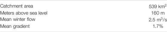
TABLE 1. Characteristics of the Sokna river (Stickler et al., 2010).

FIGURE 2

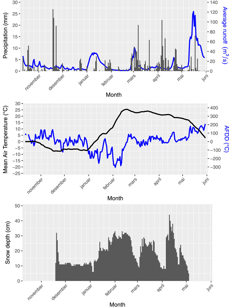
FIGURE 2. Metrological variables for the season the survey was carried out.

FIGURE 3

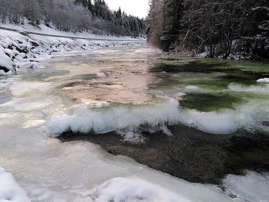
FIGURE 3. Ice Dam 1, Sokna river 5th of January 2021. Ice dam formation in progress. Picture taken at drone survey location.

Overview of Collected Data

The dataset includes drone imagery collected on 11 different days over the 2020–2021 field season. Table 2 contains the dates and ice conditions of all the drone flights considered in this paper. Table 3 contains the technical specifications of the pictures taken and the associated camera parameters. Furthermore 50 ice thickness measurements were taken on the 20th of Jan 2021. Locations of these measurements can be seen in Figure 4.

TABLE 2

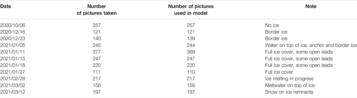
TABLE 2. Drone flights.

TABLE 3

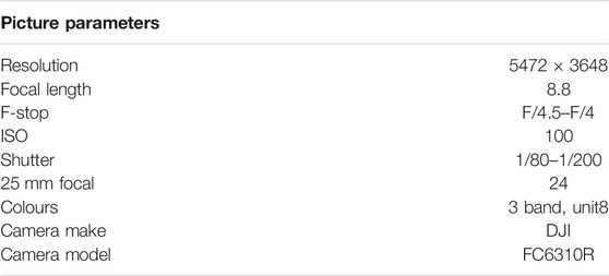
TABLE 3. Picture parameters and camera information.

FIGURE 4

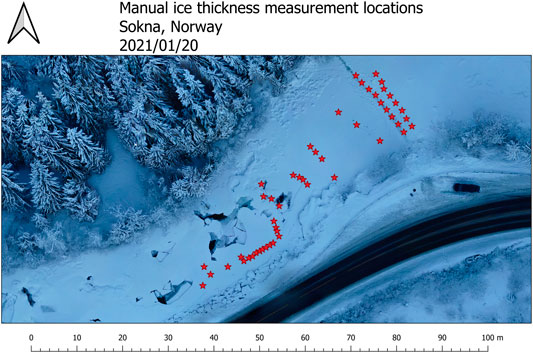
FIGURE 4. Manual ice thickness measurement locations.

Methods

Gathering Drone Imagery

A DJI Phantom 4 RTK drone was used for collecting imagery data. The drone’s location is estimated using GPS/GLONASS and corrected using CPOS. The CPOS service consists of real-time correction data received from the Norwegian Mapping Authority (Kartverket) over a 4G internet connection. The CPOS system calculates a virtual reference station (VRS) based on permanent geodetic stations and the user’s position. The drone treats data from this VRS as if it was data from a physical base station. A separate base station is therefore not required (Kartverket, 2021). The drone was flown multiple times over the study site throughout the 2020–2021 winter field season. An attempt was made to time the flights such that interesting changes in the ice cover—including no ice, freeze up, stable ice cover and breakup conditions—were captured. Furthermore, an attempt was made at avoiding adverse conditions such as glare, strong wind, fog, darkness, and rain. For each drone flight the drone took off from the same location. Due to the Norwegian drone flight regulations, the drone flight path was manually controlled with the objective of making the images cover the same area at each flight. Pictures were taken such that every picture had a minimum of 30% overlap with the previous picture. The choice of 30% overlap was based on Alfredsen et al. (2018) where ice was mapped over an area similar to the current study. The choice of overlap in the previous work was based on the experience of the drone pilot from similar SfM applications. Since the DEM of the ice surface generated by Alfredsen et al. (2018) was shown to be accurate, a similar strategy of a minimum overlap of 30% was adopted also in this project. The ice cover being mostly flat suggests that a relatively low overlap value is acceptable. The flightpath covered the area 3 times each session, once at 20 m altitude with camera pointing straight down, once at 50 m altitude with camera pointing straight down and once at 20 m altitude with camera at a 30° angle to the vertical capturing the sloping riverbank. Pictures were taken using the continuous autofocus setting, for further specification of optical parameters see Table 3.

Manual Ice Thickness Measurements

On the 20th of Jan 2021, 50 manual ice thickness measurements were made in the studied area using a Kovacs ice thickness gauge. Each measurement consisted of drilling a hole with an ice auger and then inserting the Kovacs ice thickness gauge. If the ice reached all the way to the riverbed a measuring stick was used instead. Measurement locations were chosen to ensure measurements from level ice, anchor ice dam crest, downstream of anchor ice dam crest and upstream of ice dam crest. The ice upstream of the anchor ice dam crest in the centre of the river was mostly inaccessible for manual measurement. Much of the ice cover was not manually accessible, measurements were therefore not made in a systematic grid. Major voids in the ice were subtracted from the measured ice thickness using a measuring stick where possible. See Figure 4 for ice thickness measurement locations.

Photogrammetry

The purpose of the photogrammetry step is to convert raw drone photographs into digital elevation models (DEMs) and orthomosaics. This was achieved using the proprietary software Agisoft Metashape Professional (Agisoft Metashape Professional, 2020). The following procedure—based on the procedure in (Alfredsen et al., 2018)—was adhered to:

1. Estimate image quality and discard images of quality less than 0.7

2. Align photos with accuracy “high”, discard any photos with reprojection error above 0.2

3. Build dense cloud with quality “high”

4. Build DEM

5. Build orthomosaic with hole filling enabled

Unless specified all settings were left as default (In Agisoft Metashape v1.7.0 build 11736). Note that camera alignment optimization based on Ground Control Points (GCPs) was not carried out since we used a drone with an onboard RTK-GPS. The collected GCPs were used to evaluate the accuracy of the positioning of the drone and the model. This procedure was repeated for each dataset, where each dataset consisting of all drone pictures taken of a particular location in a particular day. The output of this procedure was a pair of TIFF raster files—one DEM and one orthomosaic—for each day drone imagery was taken.

QGIS Post-processing

QGIS was used for post-processing the data (QGIS Development Team, 2009). To process the DEM raster output from Agisoft Metashape Professional, the “Ice volume” QGIS plugin was developed using the pythonic QGIS API PyQGIS and the Qt framework for the GUI. The purpose of the “Ice volume” plugin is to process river DEMs to estimate ice volume and ice thickness.

At the time of publication, the plugin takes 3 inputs:

• Path to a folder containing all .tif raster DEMs to be analysed

• Path to a .tif raster DEM with no ice and minimum water level

• Path to a .shp polygon file delineating the riverbank of the river segment

Of these all must be supplied by the user. The no ice and minimum water level raster can be acquired by flying the drone at the same site under low flow conditions with no ice and generating the rasters using SfM similarly to the ice rasters. The rasters must be overlapping and from the same location. The plugin clips all the input DEMs to the shape of the riverbank polygon. The riverbank polygon must be adjusted such that the impact of vegetation on the DEM is minimized. Without post-processing, the DEMs output by Agisoft contain spurious holes and spikes. These holes arise from insufficient number of photos, extreme reflectance values, or other optical disturbances. To remove spurious holes and spikes, Wang and Liu’s algorithm (Wang and Liu, 2006) for filling surface depressions is applied twice, once normally and once with an inverted DEM to remove spikes. This algorithm is run with a minimum slope parameter of 0.1. Then the clipped no-ice DEM is subtracted from each clipped DEM, giving difference DEMs. Statistics and transects are then calculated for the difference DEMs. The difference DEMs represent an upper bound on how thick the ice is in any given location. The described photogrammetry workflow applied to a single ∼200 picture dataset (covering an area of approximately 400 m × 100 m), run on a Dell Latitude 7,490 laptop with 16 GB of RAM and an Intel i7-8650U CPU completes in about 24 h. Most of this time is spent building the dense cloud. The QGIS post-processing run on the same laptop with the same dataset (+the no-ice basecase) completes in about 15 min.

Snow Adjustment

The drone model cannot easily tell the difference between ice and snow, nor can it easily be used to deduce the snow depth on an ice cover. A local snow depth measurement station, however, is available and its measurements are detailed in Figure 2. This snow depth is used to calculate an estimate for the snow depth on the ice cover. We assume that snow depth on ice cover is zero just after freeze-up and is set to zero whenever discharge exceeds freeze-up discharge (when this happens the snow is either flushed away or becomes snow-ice). When discharge is less than the freeze-up discharge, snow depth is assumed to change at the same rate as at the local measurement station. If this algorithm gives negative snow depth, then snow depth is set to zero. From field observations the 10th of January 2021 was set as the freeze-up date. The snow depth on the ice cover is assumed to be of uniform thickness.

Results

DEM Deviation From Control Points

To evaluate the accuracy of the DEM models, control points were recorded for 3 drone flights (2020/10/06, 2021/01/05, 2021/01/11) using a Leica VIVA GS16 RTK GPS system. For the total error the Metashape software was used to compare the model to the manually recorded control points. For these drone flights 10, 4 and 4 control points were recorded respectively, all on the banks of the river. The no-ice condition (2020/10/06) gave an average total error of 0.03 m, with a standard deviation of 0.01 m. (See Figure 10 for GCP location distribution.) The water on ice condition (2021/01/05) gave an average total error of 0.09 m, with a standard deviation of 0.03 m. The full ice cover condition (2021/01/11) gave an average total error of 0.06 m, which a standard deviation of 0.01 m. To determine altitude errors, the z-coordinate of recorded GPS points were subtracted from the z-coordinate of DEMs at the corresponding x-y coordinate. While for the total error, only control points recorded at crosshairs recognizable in the orthomosaic were used, the altitude error also used points recorded elsewhere (referred to as “other points” in Table 4). The water on ice condition (2021/01/05) gave an average altitude error of all GCPs of 0.06 m, with a standard deviation of 0.02 m. GCPs on border ice alone gave an average error of 0.06 m, with a standard deviation of 0.02 m. While points not on the border ice gave an average error of 0.06 m with a standard deviation of 0.02 m, I. e., there is no significant difference in error between border ice GCPs and on land GCPs. A Kendall rank correlation test was carried out to determine whether there is any correlation between distance from the study centre and errors. The test suggests that there is no statistically significant correlation (Kendall correlation coefficient = −0.15, Kendall test statistic = 58, p-value = 0.44). These low errors show that the precision of the RTK drone is sufficient and georeferencing using control points was not considered necessary. Errors are summarized in Table 4.

TABLE 4

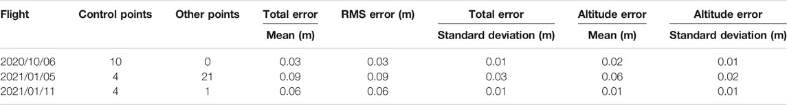
TABLE 4. Model error relative to control points.

Thickness Deviation From Manual Measurements

To evaluate the performance of the model it is instructive to consider the distribution of errors, i.e., the difference between manual ice thickness measurements and model ice thickness. For the model without hole and spike removal the errors have a mean of +21 cm and a standard deviation of 40 cm. Figure 5B shows this distribution of errors. An Anderson-Darling test (A = 0.73, p-value = 0.05) suggests that the error distribution is approximately normal. The QQ-plot (Figure 5A) suggests the same, with the caveat that the distribution has a long tail of negative errors, this tail also explains why the Anderson-Darling p-value isn’t better. Note that negative errors imply that the model predicts thinner ice than the manual measurements while positive errors imply that the model predicts thicker ice, i.e., Figure 5B suggests that the model is much more likely to overestimate ice thickness than it is to underestimate it. This is expected as the model does not consider voids or water content below the ice cover. For the model with spike and hole removal the errors have a mean of +18 cm and a standard deviation of 30 cm, i.e., no significant change in the mean, but a useful reduction in standard deviation. An Anderson-Darling test (A = 2.2, p-value < 0.001) suggests that the error distribution is no longer normal (See Figure 5C,D).

FIGURE 5

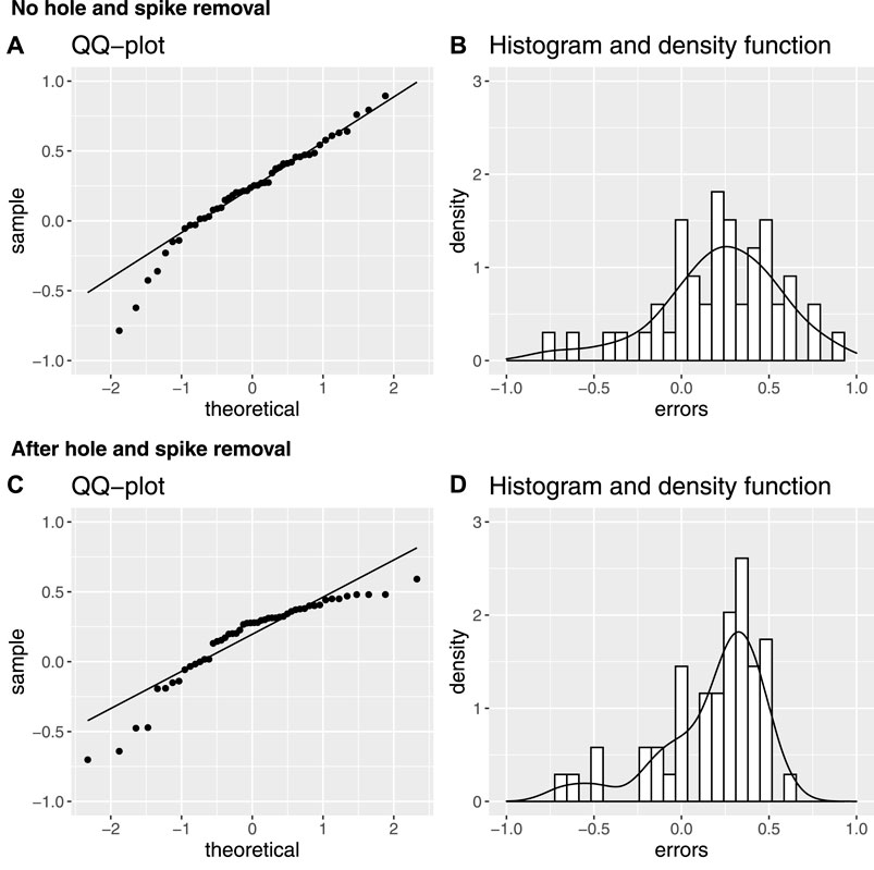
FIGURE 5. (A) Quantile-quantile plot comparing sample errors and theoretical normal errors without hole and spike removal algorithm applied. (B) Distribution of errors (Model ice thickness–real ice thickness) without hole and spike removal algorithm applied. (C) Quantile-quantile plot comparing sample errors and theoretical normal errors with hole and spike removal algorithm applied. (D) Distribution of errors (Model ice thickness–real ice thickness) with hole and spike removal algorithm applied.

DEM Temporal Trends

The drone model returns an upper bound on the ice thickness. The model is unable to estimate ice growth under a stable ice cover. This does imply that the drone model’s upper bound moves closer to the real ice thickness throughout the season as the ice thickness grows. To consider how the model ice thickness changes over time is still interesting; during freeze-up, when water flows over the ice, the model ice thickness can be expected to be a closer approximation of the true ice thickness. When a stable ice cover has been achieved any changes in ice thickness should be explainable as snow deposition, ice cover collapse or thermal expansion/contraction (or as SfM and GPS inaccuracies). In narrow rivers—such as the one studied—ice-bank adhesion is assumed to be strong enough for height differences due to water pressure to be negligible until break-up. Small changes in the model ice thickness when the ice cover is full and stable gives increased confidence in the model. To record how ice thickness varies with time, we compare ice thickness rasters for all flights. We compare them in two ways; through aggregate statistics and trough ice thickness profile comparisons. Figure 11 shows how estimated mean and median ice thickness varied during the field season. The key takeaway is that ice thickness increased rapidly in the freeze-up period, then was relatively constant throughout the rest of the season. Note the difference between the mean and the median ice thickness: the median is less affected by outliers than the average is. Ice volume can also be obtained by integrating ice thickness over the raster (this simplifies to raster area x average ice thickness). For the full ice cover condition (2021/01/18), this gives an ice volume of 8.5 × 10³ m³. Figures 6–9 show how the ice thickness at the river centreline varied through the field season. Figure 6 corresponds to drone runs where there is only border ice. Here the average centreline ice thickness hovers around zero. This is as expected since there is little ice at the centre of the river. Deviations from this are primarily errors caused by variable water level and water level opacity. The 2021/03/12 drone run in Figure 9 sometimes dips below zero thickness for the same reason. Figure 7, corresponds to the freeze-up water-on-ice condition vs. the subsequent stable ice cover condition. The difference between these two conditions shows that the drone is good at imaging anchor ice, as opposed to the water surface in this water on ice condition. The 2021/01/05 drone run therefore provides an estimate of anchor ice thickness at this time, and by extension an estimate of anchor ice volume for later runs 7.2 m³× 103 m³. In the water on ice condition, the anchor ice has not yet been fully obscured by level ice growth and is still visible through the relatively shallow water. Once the level ice has fully covered the river and the water level has dropped there will be a void in-between the underside of the level ice cover and the water/anchor-ice below. The narrow width of the river, as well as structural support from ice dam crests, mean that these suspended level ice covers and associated voids will not frequently collapse. Therefore, the water-on-ice estimate of anchor ice volume is expected to be closer to the real ice volume than equivalent estimates for full ice cover conditions. Full ice cover conditions are prone to large voids not captured by the drone imagery. Figure 8 corresponds to stable ice cover drone runs. As seen in the average/median ice thickness figure (Figure 11), the ice average thickness stays within an approximately 10 cm range throughout this part of the season.

FIGURE 6

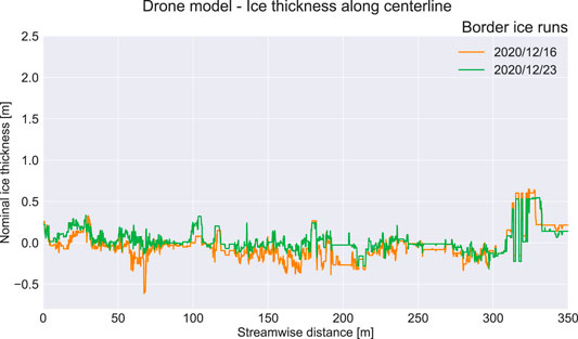
FIGURE 6. Drone model—Ice thickness along centreline for border ice drone runs.

FIGURE 7

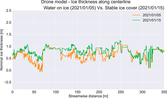
FIGURE 7. Drone model—Ice thickness along centreline for water on ice drone run.

FIGURE 8

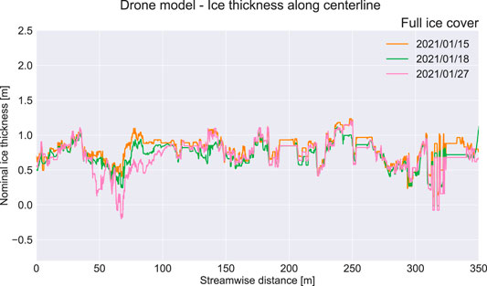
FIGURE 8. Drone model—Ice thickness along centreline for full ice cover drone runs.

FIGURE 9

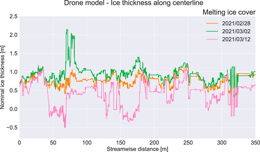
FIGURE 9. Drone model—Ice thickness along centreline for melting ice cover drone runs.

FIGURE 10

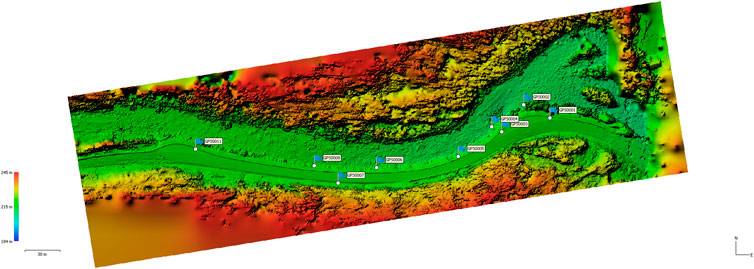
FIGURE 10. 2020/10/06 No-ice DEM with ground control points (GCPs).

FIGURE 11

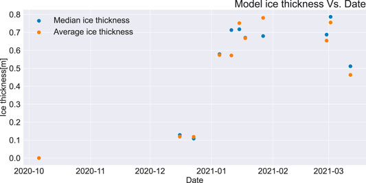
FIGURE 11. Average and median ice thickness as derived from the drone DEM model.

Discussion

A small unmanned aerial vehicle was used in combination with Structure from Motion photogrammetry to build digital elevation models of river ice during the winter season in a small stream. The use of the UAV allowed us to map the extent and estimate the volume of ice during the winter, also during conditions where traditional mapping strategies requiring access to the ice surface (Turcotte et al., 2017) would be impossible. An important feature of this method is the ability to map anchor ice dams (Turcotte and Morse, 2011), which is controlling the ice formation and hydraulic conditions in small streams like Sokna (Stickler et al., 2010). The RTK drone proved to produce accurate data and compared to ground control points measured with RTK GPS the errors were within a few centimeters. The RMS errors from this study (here they round to the same as the mean errors) are of a similar magnitude to those quoted by Alfredsen et al. (2018), who found RMS errors in the range 0.06–0.106 m. When Stott et al. (2020) mapped a small ice-free river in Scotland using comparable equipment to this study they also achieved similar RMS errors (0.066–0.072 m). Depending on lighting conditions, clarity, and depth of the water, the no-ice DEM may either represent the water surface or the riverbed. The lower the water level in the raw data for the no-ice DEM the harder this type of error is to identify by inspection as the error is small. Conversely, the deeper the water, the easier the error is to identify by inspection, but the error, however, can be much more severe. These types of errors can in principle be removed by manually eliminating the problematic areas from the analysis, however this is prone to human error and bias. The no-ice DEM should therefore ideally either be obtained through visual photography by a drone at discharges corresponding to water depth of less than 1 m (Maddock and Lynch, 2020) or optimally be obtained through lidar scanning at an appropriate wavelength for penetrating the water (Mandlburger et al., 2020). The latter method was used by Alfredsen and Juarez (2020) to integrate ice jam remnants in the river bathymetry, and hence numerically assess the impact of ice on flow patterns. Steep rivers also have an extra source of error compared to low-gradient rivers; they have higher turbulence (Wohl and Thompson, 2000), and highly turbulent water will often be captured in the DEM as solid. Furthermore, small steep rivers have rapid local changes in the water surface therefore two pictures of the same area taken in close succession may disagree on whether the water surface or the riverbed should be included in the DEM. Small steep rivers do have some advantages over big low gradient rivers: in a small river a higher percentage of the volume under the upper surface of the ice cover is ice, therefore the models’ upper bound is closer to the real value than if the same method had been applied to a big river. This makes it easier to justify using the estimates derived from the drone method for engineering purposes. If used for engineering purposes, the data should be treated as an upper bound and care should be taken not to add excessive safety factors on top of that. It should also be kept in mind that manual methods for ice thickness measurement that work well on big rivers are often inapplicable to small steep rivers. The short spans and high ice-bank adhesion in small rivers also make air-filled voids common and freeboard-based calculations unfeasible. The DEMs were cut to the riverbank, as this reduces it to the area of interest, hence removing any potential issues associated with the accuracy at the edge of the DEM, such as tall trees blocking line of sight. Vegetation overhang was a significant source of error in the first pass model. Depending on snow fall and foliage, overhanging trees will show up in the DEM as different elevations unrelated to the underlying ice thickness. These errors were however drastically reduced in the final model by inspecting the orthomosaic and cutting away any overhanging vegetation in the no-ice DEM. It is possible that some errors due to overhanging vegetation persists in later DEMs, as snow can cause vegetation to shift to new places. For DEMs of modest extent, manual inspection and removal of vegetation is likely less labour intensive and less error prone than automatic classification of the point cloud. For larger DEMs and larger data sets, automatic surface classification should be considered (Husson et al., 2016). The difference between manual ice thickness measurements and the drone model ice thickness estimates being reasonably well described by a normal or modified normal distribution suggests that it is possible to calibrate the drone model with manual measurements. I.e., use a few manual measurements to determine the mean error, then subtract that from the drone model. The drone model would then represent a best estimate of the ice thickness, rather than a conservative estimate.

Conclusion

This study was motivated by the difficulty of obtaining distributed ice thickness data in steep rivers through manual measurement. The aim of this work was to investigate the possibility of using a small drone and SfM to map the spatial and temporal distribution of ice thickness in a steep river and hence develop and evaluate a method for quantifying ice thickness distributions. The main methods used in this work were: 11 flights with a DJI Phantom 4 RTK drone at different dates for collecting imagery data, GCP points and manual thickness measurements for verification, SfM image processing using Agisoft to obtain DEMs, and a novel PyQGIS plugin for postprocessing DEMs to obtain temporal trends and quantitative statistics. This paper shows that it is possible to use a small drone and SfM to map the development of river ice in a small stream from freeze-up to break-up, including periods at the start and end where access is impossible. The work hence allows larger and more complete river ice data sets to be collected, enabling previously unfeasible analysis. High accuracy measurements of large areas of anchor ice during freeze-up is a particularly novel contribution of this paper. A model—implemented as an open source QGIS plugin—was derived for quantifying the development of ice cover by comparing digital elevation models between flights. This model showed acceptable performance for estimating ice thickness upper bounds when compared to manual measurements. The principal challenge to further develop this model includes developing better ways of estimating volume of air beneath suspended ice covers.

Data Availability Statement

Raw drone footage, environmental data, GCP coordinates and the code version current at the time of publication is available at: https://doi.org/10.5281/zenodo.5674844. For an up to date full specification of the Qgis plugin and to download it for your own use visit: https://github.com/ERodtang/ice_volume. Any other data that support the findings of this study are available from the corresponding author, ER, upon reasonable request.

Author Contributions

ER conducted most of the data collection, analysis and writing in this paper. KA supervised and provided comments on the document, discussions on the topic and help with Agisoft data processing. AJ assisted with data collection and processing of data in Agisoft. All authors contributed to the final version of the manuscript.

Funding

ER was funded by a strategic scholarship from the Norwegian University of Science and Technology (NTNU).

Conflict of Interest

The authors declare that the research was conducted in the absence of any commercial or financial relationships that could be construed as a potential conflict of interest.

Publisher’s Note

All claims expressed in this article are solely those of the authors and do not necessarily represent those of their affiliated organizations or those of the publisher, the editors, and the reviewers. Any product that may be evaluated in this article, or claim that may be made by its manufacturer, is not guaranteed or endorsed by the publisher.

Acknowledgments

The authors would like to thank Vegard Hornnes and Janik John for assistance with fieldwork.

References

Alfredsen, K., Haas, C., Tuhtan, J. A., and Zinke, P. (2018). Brief Communication: Mapping River Ice Using Drones and Structure from Motion. The Cryosphere 12 (2), 627–633. doi:10.5194/tc-12-627-2018

CrossRef Full Text | Google Scholar

Alfredsen, K., and Juarez, A. (2020). “Modelling Stranded River Ice Using LiDar and Drone-Base Models,” in The 25th IAHR International Symposium on Ice, Trondheim, November 23–25, 2020.

Google Scholar

Ansari, S., Rennie, C. D., Clark, S. P., and Seidou, O. (2021). IceMaskNet: River Ice Detection and Characterization Using Deep Learning Algorithms Applied to Aerial Photography. Cold Regions Sci. Tech. 189 (May 2020), 103324. doi:10.1016/j.coldregions.2021.103324

CrossRef Full Text | Google Scholar

Beltaos, S. (2012). Canadian Geophysical Union Hydrology Section Committee on River Ice Processes and the Environment: Brief History. J. Cold Reg. Eng. 26 (3), 71–78. doi:10.1061/(asce)cr.1943-5495.0000046

CrossRef Full Text | Google Scholar

Beltaos, S. (2008). River Ice Breakup. 1st ed. Colorado: Water Resources Publications.

Google Scholar

Beltaos, S. (1995). River Ice Jams. 1st ed. Colorado: Water Resources Publications.

Google Scholar

Beltaos, S., and Tang, P. (2013). “Applying HEC-RAS to Simulate River Ice Jams: Snags and Practical Hints,” in CGU HS Committee on River Ice Processes and the Environment, 17th Workshop on River Ice, 415–430.

Google Scholar

Bennett, K. E., and Prowse, T. D. (2009). Northern Hemisphere Geography of Ice-Covered Rivers. Hydrol. Process. 24, 235. doi:10.1002/hyp.7561

CrossRef Full Text | Google Scholar

Blackburn, J., and She, Y. (2019). A Comprehensive Public-Domain River Ice Process Model and its Application to a Complex Natural River. Cold Regions Sci. Technology. 163 (April), 44–58. doi:10.1016/j.coldregions.2019.04.010

CrossRef Full Text | Google Scholar

Carrivick, J. L., and Smith, M. W. (2019). Fluvial and Aquatic Applications of Structure From Motion Photogrammetry and Unmanned Aerial Vehicle/Drone Technology. WIREs Water. 6 (1), 1–17. doi:10.1002/wat2.1328

CrossRef Full Text | Google Scholar

Chu, T., and Lindenschmidt, K.-E. (2016). Integration of Space-Borne and Air-Borne Data in Monitoring River Ice Processes in the Slave River, Canada. Remote Sensing Environ. 181, 65–81. doi:10.1016/j.rse.2016.03.041

CrossRef Full Text | Google Scholar

Dolan, W., Yang, X., Zhang, S., and Pavelsky, T. (2019). Working towards Optical Remote Sensing of Pan-Arctic River and lake Ice. Ottawa, Ontario: CRIPE.

Google Scholar

Ewertowski, M. W., Tomczyk, A. M., Evans, D. J. A., Roberts, D. H., and Ewertowski, W. (2019). Operational Framework for Rapid, Very-High Resolution Mapping of Glacial Geomorphology Using Low-Cost Unmanned Aerial Vehicles and Structure-From-Motion Approach. Remote Sensing. 11 (1), 65. doi:10.3390/rs11010065

CrossRef Full Text | Google Scholar

Garver, J. I. (2019). “The 2019 Mid-winter Ice Jam Event on the Lower Mohawk River, New York,” in Conference: Mohawk Watershed Symposium, Schenectady, NY, March 22, 2019, 22–27.

Google Scholar

Gaffey, C., and Bhardwaj, A. (2020). Applications of Unmanned Aerial Vehicles in Cryosphere: Latest Advances and Prospects. Remote Sensing. 12 (6), 948. doi:10.3390/rs12060948

CrossRef Full Text | Google Scholar

Gebre, S., Alfredsen, K., Lia, L., Stickler, M., and Tesaker, E. (2013). Review of Ice Effects on Hydropower Systems. J. Cold Reg. Eng. 27 (4), 196–222. doi:10.1061/(ASCE)CR.1943-5495.0000059

CrossRef Full Text | Google Scholar

Husson, E., Ecke, F., and Reese, H. (2016). Comparison of Manual Mapping and Automated Object-Based Image Analysis of Non-submerged Aquatic Vegetation from Very-High-Resolution UAS Images. Remote Sensing 8 (9), 724. doi:10.3390/rs8090724

CrossRef Full Text | Google Scholar

Huusko, A., Greenberg, L., Stickler, M., Linnansaari, T., Nykänen, M., Vehanen, T., et al. (2007). Life in the Ice Lane: the winter Ecology of Stream Salmonids. River Res. Applic. 23 (5), 469–491. doi:10.1002/rra.999

CrossRef Full Text | Google Scholar

Kartverket (2021). Guide to CPOS | Kartverket.No. Available at: https://www.kartverket.no/en/on-land/posisjon/guide-to-cpos (Accessed November 12, 2021).

Google Scholar

Kääb, A., Altena, B., and Mascaro, J. (2019). River-ice and Water Velocities Using the Planet Optical Cubesat Constellation. Hydrol. Earth Syst. Sci. 23 (10), 4233–4247. doi:10.5194/hess-23-4233-2019

CrossRef Full Text | Google Scholar

Lamsters, K., Karušs, J., Krievāns, M., and Ješkins, J. (2019). Application of Unmanned Aerial Vehicles for Glacier Research in the Arctic and Antarctic. Etr. 1, 131–135. doi:10.17770/etr2019vol1.4130

CrossRef Full Text | Google Scholar

Lindenschmidt, K.-E. (2017). RIVICE-A Non-proprietary, Open-Source, One-Dimensional River-Ice Model. Water. 9 (5), 314. doi:10.3390/w9050314

CrossRef Full Text | Google Scholar

Lind, L., Nilsson, C., Polvi, L. E., and Weber, C. (2014). The Role of Ice Dynamics in Shaping Vegetation in Flowing Waters. Biol. Rev. 89 (4), 791–804. doi:10.1111/brv.12077

PubMed Abstract | CrossRef Full Text | Google Scholar

Lindenschmidt, K., Brown, D., and Hahlweg, R. (2021). “Preparing Ice-Jam Flood Outlooks for the Lower Reach of the Red River,” in 21st Workshop on the Hydraulics of Ice Covered Rivers, Saskatoon, Saskatchewan, August 29–September 1, 2021. Available at: http://cripe.ca/publications/proceedings/21.

Google Scholar

Maddock, I., and Lynch, J. (2020). Assessing the Accuracy of River Channel Bathymetry Measurements Using an RTK Rotary-Winged Unmanned Aerial Vehicle (UAV) with Varying Ground Control Point (GCP) Number and Placement. EGU Gen. Assembly. Online, EGU2020–1534. doi:10.5194/egusphere-egu2020-1534

CrossRef Full Text | Google Scholar

Mandlburger, G., Pfennigbauer, M., Schwarz, R., Flöry, S., and Nussbaumer, L. (2020). Concept and Performance Evaluation of a Novel UAV-Borne Topo-Bathymetric LiDAR Sensor. Remote Sensing 12 (6), 986. doi:10.3390/rs12060986

CrossRef Full Text | Google Scholar

Prowse, T. D., and Culp, J. M. (2003). Ice Breakup: A Neglected Factor in River Ecology. Can. J. Civ. Eng. 30 (1), 128–144. doi:10.1139/l02-040

CrossRef Full Text | Google Scholar

Smith, M. W., Carrivick, J. L., and Quincey, D. J. (2016). Structure from Motion Photogrammetry in Physical Geography. Prog. Phys. Geogr. Earth Environ. 40, 247–275. doi:10.1177/0309133315615805

CrossRef Full Text | Google Scholar

Stickler, M., Alfredsen, K. T., Linnansaari, T., and Fjeldstad, H.-P. (2010). The Influence of Dynamic Ice Formation on Hydraulic Heterogeneity in Steep Streams. River Res. Applic. 26 (9), 1187–1197. doi:10.1002/rra.1331

CrossRef Full Text | Google Scholar

Stott, E., Williams, R. D., and Hoey, T. B. (2020). Ground Control point Distribution for Accurate Kilometre-Scale Topographic Mapping Using an Rtk-Gnss Unmanned Aerial Vehicle and Sfm Photogrammetry. Drones 4 (3), 55–21. doi:10.3390/drones4030055

CrossRef Full Text | Google Scholar

Turcotte, B., Morse, B., Dubé, M., and Anctil, F. (2013). Quantifying Steep Channel Freezeup Processes. Cold Regions Sci. Tech. 94, 21–36. doi:10.1016/j.coldregions.2013.06.003

CrossRef Full Text | Google Scholar

Turcotte, B., and Morse, B. (2011). Ice Processes in a Steep River basin. Cold Regions Sci. Tech. 67 (3), 146–156. doi:10.1016/j.coldregions.2011.04.002

CrossRef Full Text | Google Scholar

Turcotte, B., Nafziger, J., Clark, S., Beltaos, S., Jasek, M., Lind, L., et al. (2017). “Monitoring River Ice Processes : Sharing Experience to Improve Successful Research Programs,” in Proceedings of the 19th Workshop on the Hydraulics of Ice Covered Rivers, Whitehorse, YK, Canada, July 10–12, 2017. Available at: http://cripe.ca/docs/proceedings/19/Turcotte-et-al-2017b.pdf.

Google Scholar

Wang, L., and Liu, H. (2006). An Efficient Method for Identifying and Filling Surface Depressions in Digital Elevation Models for Hydrologic Analysis and Modelling. Int. J. Geographical Inf. Sci. 20 (2), 193–213. doi:10.1080/13658810500433453

CrossRef Full Text | Google Scholar

Westoby, M. J., Brasington, J., Glasser, N. F., Hambrey, M. J., and Reynolds, J. M. (2012). 'Structure-from-Motion' Photogrammetry: A Low-Cost, Effective Tool for Geoscience Applications. Geomorphology 179, 300–314. doi:10.1016/j.geomorph.2012.08.021

CrossRef Full Text | Google Scholar

Wohl, E. E., and Thompson, D. M. (2000). Velocity Characteristics along a Small Step-Pool Channel. Earth Surf. Process. Landforms 25 (4), 353–367. doi:10.1002/(sici)1096-9837(200004)25:4<353:aid-esp59>3.0.co;2-5

CrossRef Full Text | Google Scholar

Woodget, A. S., Austrums, R., Maddock, I. P., and Habit, E. (2017). Drones and Digital Photogrammetry: from Classifications to Continuums for Monitoring River Habitat and Hydromorphology. WIREs Water 4 (4), 1–20. doi:10.1002/wat2.1222

PubMed Abstract | CrossRef Full Text | Google Scholar