Rapid Detection of the Change in Surface Flow Patterns Near Fish Passages at Hydropower Dams With the Use of UAS Based Videos Under Controlled Discharge Conditions

Introduction

Rivers are of great importance for both human and animal life. They represent habitats for countless riverine species and serve as sources of drinking water. They are used for transportation and recreational activities, for energy generation, as a water source in production of various goods and for irrigation purposes in agriculture.

River ecosystems are influenced by natural and anthropogenic factors (Khatri and Tyagi, 2014; Zhao et al., 2017). These factors may cause unfavourable changes in riverine environments, such as water pollution, increases in algal biomass, rapid temperature variations or dangerous changes in water depth. As a result, the ability of rivers to sustain human and animal life may be endangered. Understanding this, the scientific community across the world has been putting increasing effort into the development of methods for monitoring and assessment of river ecosystem health. One of the important research directions in this context are non-intrusive flow observation methods such as a non-contact image based surface flow measurement.

Particle Image Velocimetry, or PIV (Adrian, 2005), and Particle Tracking Velocimetry, or PTV (Agüí and Jiménez, 1987; Stegeman, 1995), the most researched and widely applied image based surface flow measurement methods, have originated in a laboratory under controlled conditions. Later they have undergone a series of adaptations in order to be used in field conditions. Other methods of non-intrusive image based surface flow measurement, such as Space-Time Image Velocimetry, or STIV (Fujita et al., 2007), Surface Structure Image Velocimetry, or SSIV (Leitão et al., 2018) and Kanade–Lucas Tomasi Image Velocimetry, or KLT-IV (Perks et al., 2016), initially targeted large-scale field applications. The use of unmanned aerial systems (UAS) as high resolution optical sensor carriers provides additional flexibility in the selection of data acquisition sites.

The advantages associated with the use of non-intrusive image based flow measurement methods in field conditions include the reduction of risks associated with data collection in dangerous flow conditions, such as flood (Fujita and Kunita, 2011; Caltrans DRISI, 2017), and the possibility of acquisition of complete instantaneous surface flow fields (Detert et al., 2017). The latter is of great importance when dealing with less typical purposes of flow data collection, such as the identification of flow patterns near fish passage entrances at hydropower dams. Flow patterns, along with flow discharges and velocities, influence the ability of fish to discover the fish passage entrance (Larinier, 2002). However, as opposed to flow velocities and discharges, flow patterns are difficult to identify by means of traditional point-based flow measurements. Image based flow measurement techniques, on the other hand, are capable of providing detailed information on complete flow fields, including both flow velocity magnitude and direction across the entire study area simultaneously.

In the current research, we identify flow patterns near a fish passage entrance at a hydropower dam by means of KLT-IV. The novelty of this research lies in the performance of measurements in controlled discharge conditions despite the large-scale format of the experiments: the river width in the study area exceeds 100 m, and the river discharge in normal conditions constitutes around 350 m³/s. We analyse three video recordings acquired at the same site with the use of the same camera sensor and the same UAS. The validation of image based measurements is performed by means of comparison with point flow velocity reference data acquired with the use of an electromagnetic flow meter. Based on the performed analysis, we identify the differences in flow patterns resulting from changing discharge conditions and discuss the advantages and the disadvantages of the non-intrusive image based approach, and KLT-IV in particular, for flow pattern identification.

Materials and Methods

Study Area and Experimental Settings

The experimental site selected for the current research (Figure 1A) is located at the foot of a hydropower dam at the River Drava in Austria. The reason for selection of the study site is its relatively large scale and the location of the fish passage entrance downstream from the obstruction at one of the river banks: this is typical for a big number of hydropower dams in Austria, which is of importance when considering the applicability of the proposed flow measurement method to other fish passage locations. In the study area, the river flows from North-West to South-East and its width varies between 100 and 130 m. The entrance into the 650 m long fish passage is located at the northern bank about 150 m downstream from the hydropower dam (see label “FP” in the Figure 1A). The elevation difference created by the dam constitutes 22 m. The river discharge at the site normally varies between 300 and 350 m³/s, while the discharge in the fish passage has values from 0.25 to 0.5 m³/s. Thus, the discharge from the fish passage normally constitutes between 0.07–0.17% of the discharge of the main flow.

FIGURE 1

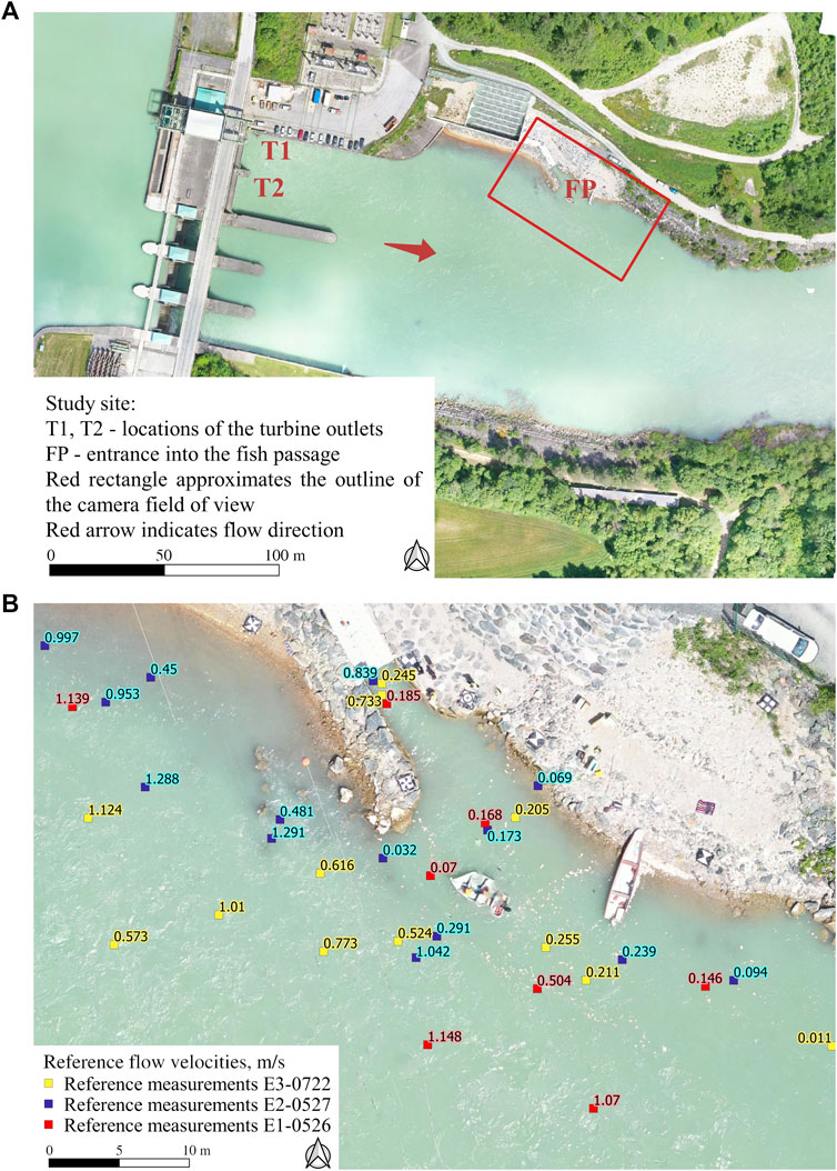
FIGURE 1. (A) An orthomosaic of the study area calculated with the use of UAS based images acquired on 26 May 2020. (B) Reference flow velocity measurements (m/s) near the fish passage entrance in three experiments.

Within the framework of this research, three experiments were conducted. The discharge conditions at the test site were controlled by changing the operation mode of the turbines of the hydropower plant and varying the discharge in the fish passage. Data collection took place at the end of spring and in summer since early spring and autumn are often characterised by high water levels in the river, which limits the possibility to freely choose the operation mode of the hydropower plant. Late spring and summer are also the most suitable seasons in terms of rare precipitation and advantageous air temperatures.

The first experiment took place on 26 May 2020. In this experiment (coded for convenience E1-0526) both hydropower plant turbines were on, producing the discharge at the dam outlet of 353 m³/s. The fish passage discharge was kept close to the lowest value at 0.255 m³/s. The video recording took place in cloudy weather conditions with a slight wind present. To account for low flow velocities near the fish passage entrance, the acquired video was sub-sampled to five fps before processing. The duration of the original video was 5 min, out of which 86 s characterised by the best tracer distribution were selected for further analysis.

The second experiment (E2-0527) took place on 27 May 2020. This time only the hydropower plant turbine located closer to the northern river bank was on, and the main flow discharge constituted 300 m³/s. The discharge in the fish passage was more than twice as high as in the first experiment (0.545 m³/s). The video recording took place in cloudy and non-windy weather conditions. As in the experiment E1-0526, the video was recorded for 5 min and sub-sampled from 25 to five fps before further processing. Out of the original video, 57 s characterised by the best tracer distribution were selected for further analysis.

The last experiment (E3-0722) was conducted on 22 July 2020. During the experiment, both turbines were off, but the residual flow led to a river discharge of 70 m³/s, while the discharge in the fish passage was set at the all-time highest value of 0.61 m³/s. The video recording took place on a sunny and non-windy day. As a result, some light reflections were present in the top right part of the field of view (FOV) during the whole video duration of 5 min. As in the previous two experiments, the video was sub-sampled from 25 to five fps before further processing. Out of the original video, 90 s characterised by the best tracer distribution were analysed. The summary of experimental settings for all three experiments is provided in Table 1.

TABLE 1

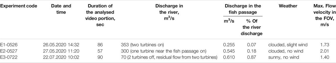
TABLE 1. Differences in discharge in the river and the fish passage in three experiments.

There were no naturally occurring suitable tracers in water at the time of data acquisition. Since the selected flow measurement method relies on the presence of traceable particles in the flow, the required tracers were introduced into the flow manually. Natural ecofoam chips of blue, pink and yellow colours were selected as tracers for the following reasons:

• they are produced from corn starch and are therefore biodegradable, which prevents water pollution;

• their application in previous image based flow measurements has shown that in low wind conditions they accurately describe the surface flow (Dramais et al., 2011; Sutarto, 2015; Strelnikova et al., 2020);

• they have good contrast with the background and are easy to visually identify;

• they have low cost, which is essential in large-scale field experiments, associated with the high volume of the necessary tracer material.

Data acquisition was performed with the help of a 4K Zenmuse X5R camera set at a frame rate of 25 fps and an image resolution of 3840 x 2160 px. As a camera carrier platform, we used a DJI based hexacopter ViewCopter V6 Heavy assembled in Austria (empty mass 7 kg, maximum take-off mass 16 kg; flight time, depending on payload: 15–25 min), which has proven to have high stability in windy conditions. Further improvement of positioning stability of the UAS was achieved by means of using a real time kinematic (RTK) positioning system. In all three experiments, the UAS flight height was set to 75 m above the water level resulting in a ground sampling distance of about 2 cm, enabling easy visual recognition of individual tracers. Though a higher flight altitude would allow to increase the captured area which could be of interest when dealing with even larger rivers, it would likely have a negative impact on the visibility of individual tracers and small tracer clusters, unless tracers of larger size are used. This in turn could negatively influence the accuracy of image-based flow measurement.

Due to a large river width, the FOV used for data acquisition included only the area around the fish passage entrance; the southern river bank was left outside the FOV. All ground control points (GCPs) in the FOV were located along the northern river bank. Black-and-white plastic plates with the dimensions of 0.8 × 0.8 m served as GCP markers. The contrast between the GCP markers and the background was increased by placing pieces of black pond liner underneath the GCP markers. The positions of GCP marker centres were determined with the use of a differential GPS with an accuracy of ±3 cm.

Image Velocimetry With the Use of KLT-IV

Image based velocimetry relies on measuring the displacement of traceable features between the individual images in an image sequence. When images in the sequence are recorded at a constant rate, as in a case of video frames, it is possible to derive the velocity of traceable feature movement in pixels per frame. For the calculated velocities to be comparable to each other, the area of interest for which the velocities are calculated must be characterised by a constant relationship between the image units and the real-world units, that is to have a constant scale. If the frame rate and the scale are known, the velocities calculated in px/frame can be converted into real-world units, e.g. m/s.

The Kanade–Lucas–Tomasi (KLT) algorithm (Shi and Tomasi, 1994) is an established way of feature detection and tracking. Perks et al. (2016) demonstrated that this algorithm can be used for image based velocimetry purposes and later, Pearce et al. (2020) demonstrated the performance of KLT-IV for velocity measurements in low flow conditions. The KLT-IV software (Perks, 2020) represents a suite which, in addition to performing the actual image velocimetry, includes such functions as image orthorectification and stabilisation, as well as discharge calculation. KLT-IV is a free compiled Matlab application. In order to be able to run it, it is sufficient to have the freely available Matlab Runtime installed.

The following minimum data input are required to perform image velocimetry analysis with the use of KLT-IV software:

• a video recording of the flow with visually identifiable traceable features (usually from 30 s up to several minutes in length);

• an initial estimate of the 3D location (x, y, z; in metres) and an orientation of the camera sensor during data acquisition;

• Accurate 3D locations (x, y, z; in metres) of GCPs and the corresponding locations of GCPs in the image space in pixels;

• A defined FOV within which analysis will be undertaken. This can be presented as either minimum and maximum x and y values in metres or as a buffer value around the given GCPs;

• water level in metres.

KLT-IV software allows an easy export of the calculated velocity values in CSV format for further analysis as well as plotting the calculated trajectories of traceable features. These trajectories are colour-coded with respect to the corresponding velocities. The software can also plot the trajectory of the camera carrier platform, usually a UAS, which took place during the video recording. If such movement is present, it can be automatically compensated for by means of an image stabilisation option. KLT-IV performs image orthorectification based on the initial location and orientation of the camera and the GCP data, as well as on an optionally provided camera type from a pre-defined list of commonly used camera sensors, which is used to compensate for various lens distortions, such as a barrel distortion. There is an option of exporting orthorectified images when necessary.

The publicly available version of the KLT-IV software includes no image pre-processing options and no possibility to upload custom camera parameters required for the removal of lens distortions. Therefore, lens distortions characteristic for the Zenmuse X5R camera used in the current research were removed beforehand using Matlab and the Camera Calibrator app (Bouguet, 2015).

Visualisation of image velocimetry results was performed by means of the standard velocity plotting functionality of the KLT-IV software. A standard scale from 0 to 2 m/s was used for velocity plotting in all three experiments despite the differences in maximum velocities within the FOV in order to enable an objective visual comparison between all three surface velocity fields.

Validation of Image Velocimetry Results

Reference measurements intended to be used for the validation of image based flow analysis results were conducted using a bi-axial electromagnetic E-40 probe combined with a P-EMS control unit, a programmable four-quadrant electromagnetic liquid velocity meter produced by Delft Hydraulics. The locations of reference flow velocity measurements were determined with the use of a differential Global Navigation Satellite System (GNSS) with an accuracy of ±3 cm. Reference flow velocities were measured from a boat at different locations: (1) near the entrance into the fish passage, (2) downstream from the fish passage entrance in the vicinity of the northern river bank and (3) in the main flow near the fish passage entrance. Each measurement was performed directly underneath the water surface. Flow velocities in each location were recorded for 1 min, after which all the acquired values were averaged and standard deviations were calculated. A total of eight reference velocities were acquired in the course of 24 min during the experiment E1-0526 (red markers in Figure 1B, 14 reference velocities were measured in the course of 26 min during the experiment E2-0527 (blue markers in Figure 1B and 12 reference velocities were acquired in the course of 27 min during the experiment E3-0722 (yellow markers in Figure 1B).

After performing image velocimetry by means of the KLT-IV software, the exported velocities were compared to reference measurements collected in the field. For each reference measurement, the following was performed. First, we selected all the velocity vectors calculated with the use of KLT-IV within the radius of 0.25 m around the location of each reference measurements. Then, the KLT-IV vectors corresponding to each of the reference measurements were used to calculate the mean velocity magnitude and standard deviation. The number of available velocity vectors varied greatly between locations depending on the density of tracer particles within the region of interest (ROI). The minimum number of available velocity vectors for a reference measurement location was 4 (in the experiment E2-0527), and the maximum number of available velocity vectors was 1217 (in the experiment E3-0722). The median number of KLT-IV velocity vectors per reference measurement location was 63.

The comparison between the reference measurements and the KLT-IV velocities was performed with consideration of uncertainties available in the form of one standard deviation from the mean velocity magnitude values. Since reference measurements were available as points distributed within the FOV and not as a cross-section, for the visual representation of comparison between the reference velocities and the analysis results, the reference velocities were sorted according to their magnitude.

Results

Experiment E1-0526: High Main Flow Discharge, Low Fish Passage Discharge

Despite the intention to perform data acquisition at nadir, the actual camera angle during video recording slightly differed from the intended one. The visual representation of surface flow velocity fields calculated by means of KLT-IV is given in Figure 2. Dark-blue lines running from North-West to South-East in the middle of the Figure 2 represent an artefact resulting from the presence of the power cables within the FOV. The maximum calculated flow velocity magnitude in the FOV was as high as 1.73 m/s. The reference velocities available for the validation of KLT-IV results ranged from 0.070 to 1.148 m/s, however, none of the reference measurements were located in the area characterised by the highest flow velocities according to KLT-IV.

FIGURE 2

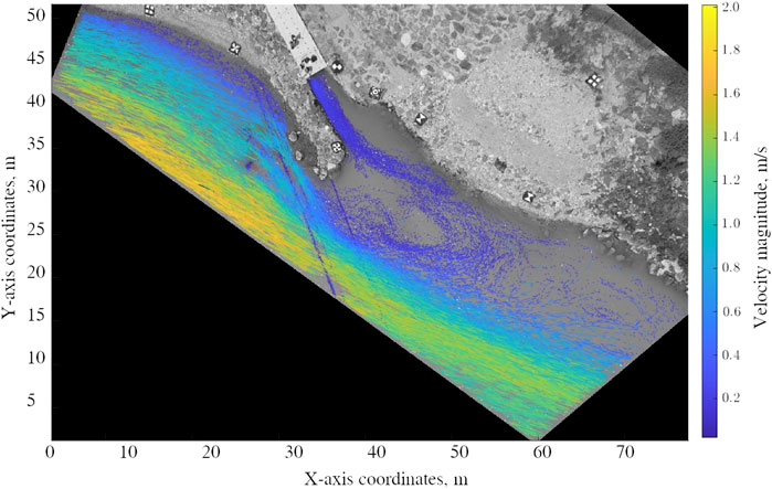
FIGURE 2. The visualisation of surface flow patterns near the fish passage entrance in the experiment E1-0526. Dark-blue lines running from North-West to South-East in the middle of the image represent an artefact resulting from the presence of the power cables within the FOV.

The comparison of reference velocities with the KLT-IV results is presented in Table 2 and visualised in Figure 3. The mean KLT-IV values tend to be slightly higher than the mean reference velocities. However, all reference measurements lie within the one standard deviation uncertainty interval of the corresponding KLT-IV results and vice versa. Reference velocity measurements are characterised by higher standard deviation values than KLT-IV results. Thus, the calculated uncertainties associated with KLT-IV mean velocities are less in comparison to the uncertainties associated with the reference measurements.

TABLE 2

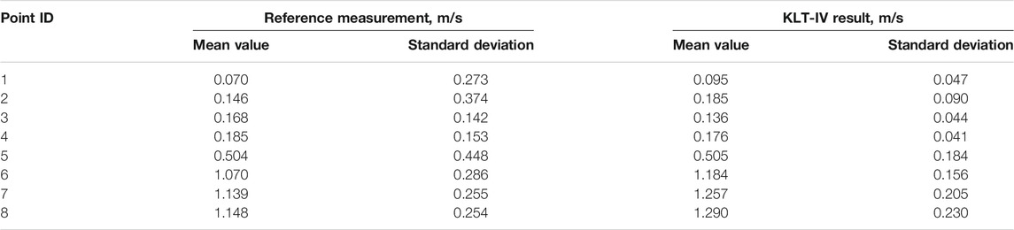
TABLE 2. Comparison of mean velocity magnitudes and standard deviations between the reference measurements and the KLT-IV analysis results in the experiment E1-0526.

FIGURE 3

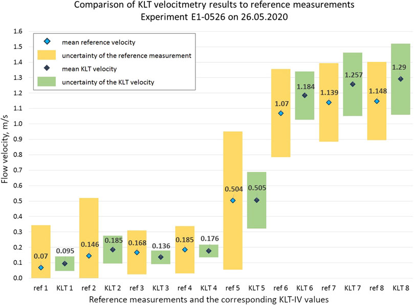
FIGURE 3. The comparison of reference velocity measurements with the KLT-IV results calculated in the experiment E1-0526.

Experiment E2-0527: High Main Flow Discharge, High Fish Passage Discharge

In the second experiment, data acquisition was performed at nadir. The visual representation of surface flow velocity fields calculated by means of KLT-IV for the experiment E2-0527 is given in Figure 4. The artefact in the left bottom corner of the FOV is related to the presence of the power cables within the FOV; it is displaced from its original position in the experiment E1-0526 due to a change in the UAS location and camera angle. The maximum calculated flow velocity magnitude in the FOV was as high as 2.01 m/s. None of the reference measurements were located in the area characterised by the highest flow velocities according to KLT-IV. The reference velocities available for the validation of KLT-IV results ranged from 0.032 to 1.291 m/s.

FIGURE 4

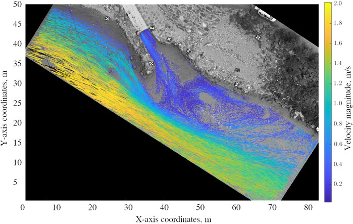
FIGURE 4. The visualisation of surface flow patterns near the fish passage entrance in the experiment E2-0527. The artefact in the left bottom corner of the image is related to the presence of the power cables within the FOV.

The comparison of reference velocity measurements for the experiment E2-0527 with the KLT-IV results is presented in Table 3 and visualised in Figure 5. In over 60% of the cases (9 of 14 measurements), the mean KLT-IV values are slightly higher than the mean reference velocities. At the same time, most reference measurements lie within the one standard deviation uncertainty interval of corresponding the KLT-IV results. In one case the reference measurement lies outside the KLT-IV uncertainty interval, below its lower boundary, whereas the KLT-IV result is still within the uncertainty interval of this reference measurement. Reference velocity measurements are, with one exception, characterised by higher standard deviation values than KLT-IV results.

TABLE 3

TABLE 3. Comparison of mean velocity magnitudes and standard deviations between the reference measurements and the KLT-IV analysis results in the experiment E2-0527.

FIGURE 5

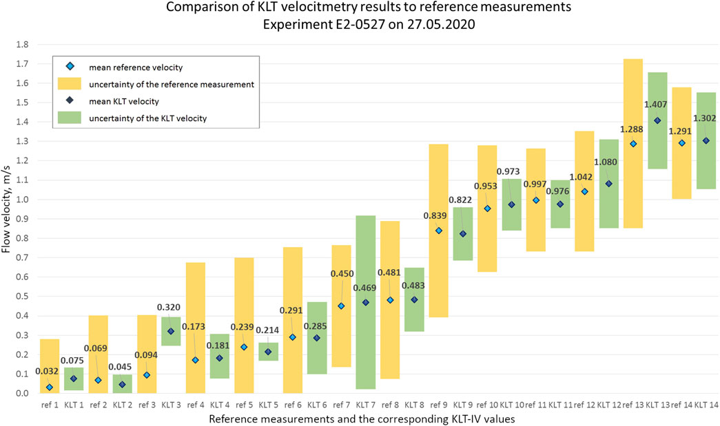
FIGURE 5. The comparison of reference velocity measurements with the KLT-IV results calculated in the experiment E2-0527.

Experiment E3-0722: Low Main Flow Discharge, High Fish Passage Discharge

In the third experiment, as in the experiment E2-0527, data acquisition was performed at nadir. The proportion of the water surface present in the FOV was slightly greater compared to the previous two experiments. The visual representation of surface flow velocity fields calculated by means of KLT-IV for the experiment E3-0722 is given in Figure 6. As in the experiment E2-0527, power cables produce an artefact in the left bottom corner of the FOV. The maximum calculated flow velocity magnitude in the FOV was as high as 1.40 m/s. The reference velocities available for the validation of KLT-IV results ranged from 0.011 to 1.124 m/s.

FIGURE 6

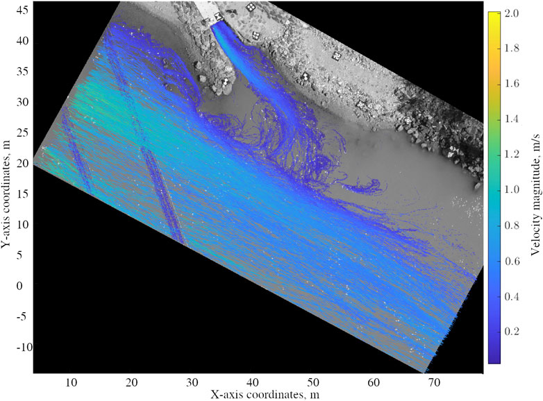
FIGURE 6. The visualisation of surface flow patterns near the fish passage entrance in the experiment E3-0722. The artefact in the left bottom corner of the image results from the presence of the power cables in the FOV.

In the top right corner of the water surface in the experiment E3-0722, downstream from the last reference measurement of 0.011 m/s, almost no tracers were observed in the analysed portion of the video. At the same time, direct sunlight reflections were present in this area. Such reflections constitute a part of the image noise and negatively influence the performance of image-based velocimetry algorithms since the behaviour of the reflections is not representative of the flow while algorithms regarded them as traceable features (Detert and Weitbrecht, 2016; Dal Sasso et al., 2018). In order to avoid false velocity calculation in the top right corner of the water surface with direct sunlight reflections, this area was excluded from ROI during analysis.

The comparison of reference velocity measurements for the experiment E3-0722 with the KLT-IV results is presented in Table 4 and visualised in Figure 7. In the majority of the cases (8 of 12 measurements), the mean reference velocity values are slightly higher than the KLT-IV mean velocities. Most reference measurements, with one exception, lie within the one standard deviation uncertainty interval of corresponding the KLT-IV results. All KLT-IV results lie within the one standard deviation uncertainty interval of the reference measurements. All reference velocity measurements are characterised by higher standard deviation values than KLT-IV results.

TABLE 4

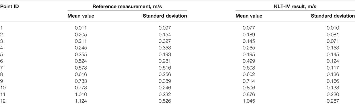
TABLE 4. Comparison of mean velocity magnitudes and standard deviations between the reference measurements and the KLT-IV analysis results in the experiment E3-0722.

FIGURE 7

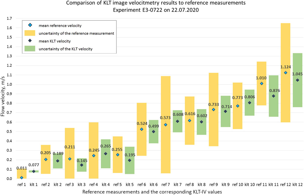
FIGURE 7. The comparison of reference velocity measurements with the KLT-IV results calculated in the experiment E3-0722.

Discussion

The results of KLT-IV analysis show that flow patterns near the entrance into the fish passage observed in three experiments under controlled discharge conditions experience both commonalities and differences. The first obvious difference is the distribution of surface flow velocities in the ROI. In the experiment E1-0526, the discharge from the fish passage entrance was the lowest (0.255 m³/s), and this is reflected in a narrower and slower flow from the fish passage entrance appearing in the Figure 2 when compared to the following two experiments (Figures 4, 6). The fish passage discharge values in the experiments E2-0527 and E3-0722 were greater than in the first experiment, 0.545 m³/s and 0.610 m³/s respectively, which led to more similarities in flow velocities near the fish passage entrance between the experiments E2-0527 and E3-0722 compared to E1-0526. The highest discharge from the fish passage entrance in E3-0722, as expected, was associated with the highest flow velocity, and this was correctly reflected by the flow patterns calculated with the help of KLT-IV (Figure 6).

In all three experiments, the identified flow from the fish passage entrance was more pronounced along the breakwater-like rocky structure since this is the side of the opening in the fish passage entrance, as one can see in Figure 8. This constructional peculiarity leads to a formation of a strong flow along breakwater-like structure heading into the downstream direction. At the same time, a backflow is formed along the bank heading into the opposite direction, towards the fish passage entrance.

FIGURE 8

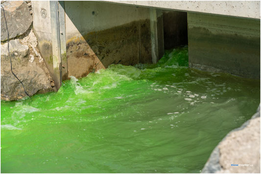
FIGURE 8. An entrance into the fish passage.

In E1-0526, the flow from the fish passage looks narrower than in the other two experiments. This is explained by the fact that there is very little backflow along the river bank in this experiment compared to experiments E2-0527 and E3-0722 because of the significantly lower discharge from the fish passage, resulting in a lower flow velocity. In the experiments E2-0527 and E3-0722, the flow near the fish passage entrance along the river bank represents the backflow, though is not obvious from the Figures 4, 6 since the Figures do not contain visual information about flow directions. It could be of benefit for the users of future versions of the KLT-IV software to have an option of plotting flow directions in addition to colour-coded tracer trajectories.

In all three experiments, mean velocities of the flow from the fish passage entrance were close to the reference measurements:

• E1-0526: 0.185 m/s [ref]/0.176 m/s [KLT-IV];

• E2-0527: 0.839 m/s [ref]/0.822 m/s [KLT-IV];

• E3-0722: 0.733 m/s [ref]/0.714 m/s [KLT-IV] (lower reference value compared to the experiment E2-0527 may be attributed to the fact that the measurement was performed further away from the fish passage entrance than in the experiment E2-0527, as well as to the turbulent nature of the high flow in the close proximity of the fish passage entrance);

• In the experiment E3-0722, additionally to the velocity of the flow from the fish passage entrance, the velocity of the backflow was measured: 0.245 m/s [ref]/0.265 m/s [KLT-IV].

In all three experiments, velocities of the flow from the fish passage calculated with the use of KLT-IV were slightly lower than the reference velocities. At the same time, the velocity of the backflow in the experiment E3-0722 calculated with the use of KLT-IV, was slightly higher than the corresponding reference value. This may be related to the fact that tracer particles were added into the flow from the fish passage entrance directly from above its opening, producing large unstable clusters of tracers within the flow from the fish passage entrance, whereas in the backflow individual tracers were more distinct and easier to track.

The highest velocities in the ROI were, as expected, observed within the main flow in the experiment E2-0527 (2.0 m/s). River discharge values in the experiments E1-0526 and E2-0527 were similar to each other, with a slightly lower main flow discharge value in the experiment E2-0527 (300 m³/s vs. 353 m³/s in E1-0526). However, in the experiment E2-0527 only the turbine T1 near the Northern river bank was in operation, whereas in the experiment E1-0526 the discharge was distributed between the outlets of both turbines T1 and T2. Since the turbine T1 is the one having the greater influence on flow patterns within the FOV, increasing the discharge from its outlet produced a stronger flow closer to this river bank and to the fish passage entrance. In the experiment E1-0526, where about half of the total discharge of 353 m³/s was attributed to the turbine T1, the velocity of the main flow near the fish passage entrance was lower. KLT-IV based flow patterns depicted in Figures 2, 4 correctly reflect these differences. The lowest main flow velocities were associated with the settings of the experiment E3-0722 characterised by the lowest main flow discharge (70 m³/s) distributed between two turbine outlets, which can be seen in Figure 6.

In the experiments E1-0526 and E2-0527, velocities calculated by means of KLT-IV were slightly higher than the majority of reference measurements, whereas in the experiment E3-0722 reference velocities tended to be greater than the ones calculated with the help of KLT-IV. This may be because the first two experiments were characterised by higher main flow discharge and waves were visible on the water surface. These waves were not filtered out before flow velocity calculation since the recorded video frames were used for the analysis “as is”, without preliminary image enhancement. As such, these waves comprised a part of traceable features and could influence the surface flow velocity calculation. In the last experiment, there were almost no waves visible within the ROI, and thus flow velocities were calculated solely based on the movement of artificially introduced tracers.

In all three experiments, the flow from the fish passage entrance joined the main flow at a distance of between 21 and 25 m. However, the behaviour of the flow on the way to the main flow was different. Box plots of flow velocities near the fish passage entrance in all three experiments are juxtaposed to each other in Figure 9.

FIGURE 9

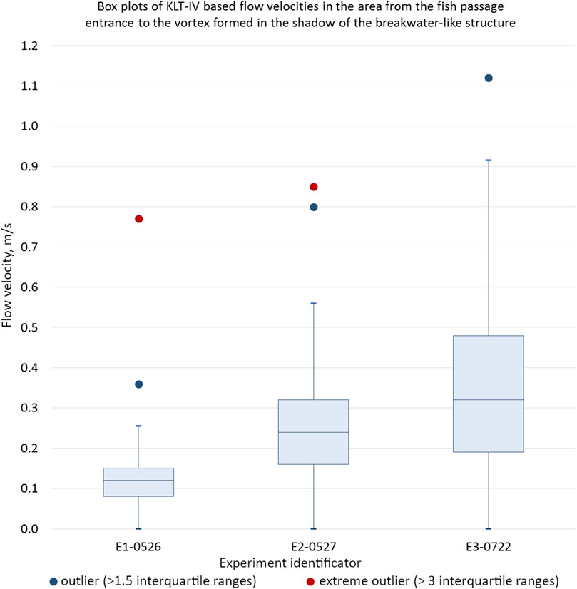
FIGURE 9. Box plots of KLT-IV based flow velocities in the area from the fish passage entrance to the vortex formed in the shadow of the breakwater-like structure.

In the experiment E1-0526, the flow from the fish passage had the lowest velocity and tended to move closer to the river bank. In the shadow of the breakwater-like structure a vortex was formed, and the flow from the fish passage joined the main flow within this vortex. The velocity of the flow from the fish passage entrance downstream to this vortex was relatively constant, reaching up to 0.255 m/s. About 1.03% of all calculated velocity values lied over this upper limit and constituted statistical outliers (values up to 0.36 m/s), whereas 0.05% of all calculated values belonged to extreme outliers (values up to 0.77 m/s). The median flow velocity and the mean flow velocity were almost identical and constituted 0.120 m/s and 0.117 m/s respectively.

In the experiment E2-0527, the flow from the fish passage entrance was much stronger than in the previous experiment, which was expected due to the doubled discharge value. A high standard deviation associated with the reference velocity of the flow from the fish passage entrance (mean velocity 0.839 m/s, standard deviation 0.447 m/s) indicated that the flow from the fish passage was characterised by high turbulence. The flow from the fish passage was directed from North-West to South-East straight into the main flow, not along the bank as in the experiment E1-0526. A vortex was formed in this experiment, too. In this case, however, it was observed directly after at the location where the flow from the fish passage joined the main flow. In their majority, flow velocities near the fish passage entrance calculated with the use of KLT-IV did not exceed 0.560 m/s; however, some of the calculated velocities directly near the opening of the fish passage reached as high as 0.800–0.850 m/s, which from the statistical point of view represented outliers. The outlier values constituted 2.83% of all velocities calculated near of the fish passage entrance; extreme outliers, namely the values above 0.800 m/s, constituted 0.07% of all calculated velocity vectors. Considering the fact that the reference mean flow velocity measured in this experiment directly near the opening of the fish passage entrance was equal to 0.839 m/s, it is likely that though high KLT-IV mean velocities in this area represent outliers from the statistical point of view, they have not resulted from a calculation error but rather reflect the actual mean flow velocities in this small region directly near the fish passage entrance.

As in the experiment E1-0256, also in the experiment E2-0527 the mean and the median velocity values within the flow from the fish passage entrance (excluding the backflow) were similar to each other. At the same time, their values were twice as high as in the experiment E1-0526 and constituted 0.250 m/s and 0.240 m/s respectively. These values reflected the change in the discharge from fish passage entrance from 0.255 m³/s to 0.545 m³/s.

In the last experiment, E3-0722, the discharge from the fish passage entrance was increased by about 12%, from 0.545 m³/s to 0.610 m³/s. This discharge value lead to a situation when some of the fish passage pools were close to being overfilled, such that further increase in discharge was impossible. The observed relative change in flow velocities directly near the fish passage entrance was more pronounced than the relative change in the discharge value. The mean and the median velocity values for the flow from the fish passage entrance (excluding the backflow) constituted 0.345 m/s and 0.320 m/s respectively, which represented an increase by over 30% compared to the experiment E2-0527. Overall, flow velocities near the fish passage entrance reached up to 0.915 m/s, with some outliers up to 1.120 m/s, whereas these statistical outliers constituted only 0.29% of all calculated velocity values in the area. Among these, no extreme outliers were observed.

Interestingly, the flow from the fish passage entrance did not follow the shortest way into the main flow as in the experiment E2-0527 but went closer to the river bank. A vortex was formed between the breakwater-like structure and the location where the flow from the fish passage joined the main flow. Due to this phenomenon, in the experiment E3-0722 the flow from the fish passage entrance joined the main flow at an angle of about 70°, whereas in the experiment E2-0527 this angle was more acute, about 45°. For the discoverability of the fish passage entrance, the lesser angle, as in the experiment E2-0527, is considered to be more beneficial (Larinier, 2002). Together with the fact that in both experiments E2-0527 and E3-0722 the flow from the fish passage entrance had almost identical reach into the main flow, it must be concluded that the flow pattern induced near the fish passage entrance in the experiment E2-0527 was preferable over the flow pattern in the experiment E3-0722, despite the fact that the discharge from the fish passage in E2-0527 constituted 0.18% of the river discharge as opposed to 0.87% in the experiment E3-0722. This comparison demonstrates that specifying an attraction flow necessary for the discoverability of a fish passage as dependent solely on its relative discharge in comparison to the discharge of the main flow is an oversimplification, and that fish passage design must be viewed as a more complex optimization problem (Gisen et al., 2017). Other factors, including actual flow patterns induced near the fish passage entrance in current discharge conditions, must be taken into account when accessing fish passage discoverability.

In all three experiments, most of the uncertainties associated with KLT-IV mean velocities calculated as one standard deviation from the mean value were less in comparison to the uncertainties associated with the reference measurements. The reference measurements are likely to have large variability due to pulsed and turbulent flows, which is reflected in the measurements of the flow meter as a large standard deviation. This variability is likely to be reduced by KLT-IV since it tracks feature displacements for several frames (corresponding to, e.g., 1s of the video duration) and only then calculates the velocity based on the length of the restored feature path and the time it took to displace the feature along this path. In this way, small scale accelerations/decelerations get averaged over the path, reducing the variability of the results. Another meaningful factor is that the locations of velocity vectors calculated by the KLT-IV depend on the distribution of traceable features, and as such they must not exactly correspond to the locations of the reference measurements. For this reason, standard deviations calculated for the mean KLT-IV velocities are based on all velocities within a 0.25 m radius around the location of the reference measurement, not in a single point. When several velocity vectors are calculated within such a small area, they are likely to be similar to each other due to the described averaging mechanism of the KLT-IV, and this similarity is likely to contribute to the reduction of the standard deviations associated with the KLT-IV measurements.

Previous studies (Pearce et al., 2020) demonstrated that KLT-IV may be sensitive to feature extraction rate in low flow conditions. In the experiments comprising the current research, the largest absolute difference between the mean reference velocity and the corresponding KLT-IV result was observed in the experiment E2-0527 and comprised of 0.226 m/s for the reference velocity 0.094 m/s, whereas the KLT-IV result was 0.320 m/s. The largest relative differences between the mean reference velocities and the corresponding KLT-IV results were observed in the areas where flow velocities lied below 0.10 m/s. Thus, it is likely that the frame rate of five fps is not optimal for measuring the flow by means of KLT-IV in the areas with velocities lower than 0.10 m/s, which considering the ground sampling distance of around 2 cm constitutes less than one px/frame.

The best correspondence between the reference values and KLT-IV results were observed in the velocity range from 0.291 m/s to 0.997 m/s (which roughly corresponds to 3–10 px/frame). Here, absolute differences between the calculated and the reference mean flow velocities ranged from −0.035 m/s to +0.025 m/s; in relative terms, the differences lied between −6.11% and +4.77%.

Overall, flow velocities calculated with the use of KLT-IV in three experiments corresponded to the available reference measurements: out of 34 available reference velocity values, 32 lied within the one standard deviation uncertainty interval of the corresponding KLT-IV mean velocity. Therefore, image-based flow pattern analysis with the help of KLT-IV represents a promising alternative approach to deriving flow patterns when compared to the complicated hydraulic modelling based on point flow velocity values.

The difficulties associated with the application of the non-contact KLT-IV flow measurement method include the necessity to introduce artificial tracers into the flow in the absence of naturally occurring traceable features, which can be challenging and cost-intensive in the case of large rivers. Further, as with all image-based methods, the quality of the recorded video data is of crucial importance. Environmental noise, such as light reflections and shadows, leads to a false flow velocity calculations, resulting in a creation of spurious velocity vectors (Hauet et al., 2008; Dal Sasso et al., 2018). Windy weather conditions lead to a creation of waves which are not representative of the actual flow but get included into traceable features, thus reducing the quality of image-based analysis. Moreover, when a UAS is used as a camera carrier platform, data capture in windy conditions may further reduce the quality of acquired videos or may be overall impossible due to a high risk of equipment damage. Also, a video recorded in windy conditions tends to be shaky and not easy to stabilise, which significantly increases the video pre-processing effort. Thus, it is advisable to capture data in non-windy weather conditions whenever possible.

Data collection in the described study took place at the end of spring and in summer characterised by rare precipitation and air temperatures suitable for the operation of equipment used in data capture. In winter, data acquisition may be complicated by very low temperatures, below the operating limits of the equipment. Precipitation may lead to the equipment damage or create noise on the water surface, making further application of image-based flow analysis methods impossible. Therefore, it is advisable to perform data collection when there is no precipitation, paying attention to the correspondence between the air temperature and the operational requirements of the employed equipment.

In the absence of strong environmental noise, when there are naturally occurring traceable features in the flow or when there is a possibility to use artificial biodegradable tracers, KLT-IV provides a fast and reliable non-contact method of deriving flow patterns from video recordings acquired with the use of UAS in field conditions.

Conclusion

This study has compared flow patterns calculated based on the video data acquired in three field experiments. All experiments were conducted at the same location near a fish passage at a hydropower dam at the River Drava in controlled discharge conditions. A non-contact image-based flow measurement method KLT-IV was used for surface flow pattern calculation. The validation of the analysis results was performed by means of their comparison with the reference mean flow velocities acquired in the field with the use of an electromagnetic current meter. The validation has shown that in 94% of all cases reference mean flow velocities lied within one standard deviation uncertainty interval from the mean velocity value calculated by means of KLT-IV.

Due to a higher main flow discharge in the first two experiments, visible waves were present on the water surface, whereas in the last experiment only the movement of artificial tracers could be observed. Weather conditions were not exactly identical either: the first experiment was characterised by a slight wind, and in the last experiment the weather was sunnier compared to the previous two experiments. Such environmental effects can be accounted for at the image enhancement stage of data processing. Introduction of image enhancement functionality into the future versions of the KLT-IV software may be beneficial when dealing with noisy video data.

The best correspondence between the reference measurements and KLT-IV results were observed in the flow velocity range from ∼0.3 m/s to ∼1 m/s, which roughly corresponds to 3–10 px/frame. The calculated flow patterns have confirmed expected changes in hydraulic conditions caused by changing discharge values, e.g. an increase in velocity from the fish passage entrance when the corresponding flow discharge was increased. At the same time, some unexpected findings were observed. For example, further increase in discharge from the fish passage did not benefit the resulting flow pattern since it unfavourably changed the angle at which the flow from the fish passage joined the main flow. This finding underlines the importance of developing a methodology which helps to quickly identify the changes in flow patterns in the light of changing discharge conditions in order to be able to increase the fish passage discoverability at peak times of fish migration. The performance of the KLT-IV algorithm in this study and the availability of the free-to-use KLT-IV software show that KLT-IV can represent a promising solution when there is a need to quickly identify the change in surface flow patterns.

Data Availability Statement

The datasets used in this study will be provided by the corresponding author upon request.

Author Contributions

HM, GP, DS, SK, K-HA, PM contributed conception and design of the study; DS wrote the first draft of the manuscript; MTP wrote sections of the manuscript and performed several reviews; US and RS performed UAS-based data acquisition; PM collected ground truth data. All authors contributed to manuscript revision, read and approved the submitted version.

Funding

This research has been partially funded by Verbund Hydro Power GmbH. The publication of this research has been supported by the European Cooperation in Science and Technology (COST Action; grant no. CA16219; “HARMONIOUS–Harmonization of UAS techniques for agricultural and natural ecosystems monitoring”).

Conflict of Interest

All authors except for MTP have financial relationships with Verbund Hydro Power GmbH due to its partial funding of this research. Verbund Hydro Power GmbH does not sell flow measurement software, equipment or services. MTP is the developer of freely available KLT-IV software. MTP has no commercial or financial relationships with Verbund Hydro Power GmbH.

Publisher’s Note

All claims expressed in this article are solely those of the authors and do not necessarily represent those of their affiliated organizations, or those of the publisher, the editors and the reviewers. Any product that may be evaluated in this article, or claim that may be made by its manufacturer, is not guaranteed or endorsed by the publisher.

References

Adrian, R. J. (2005). Twenty Years of Particle Image Velocimetry. Exp. Fluids 39, 159–169. doi:10.1007/s00348-005-0991-7

CrossRef Full Text | Google Scholar

Agüí, J. C., and Jiménez, J. (1987). On the Performance of Particle Tracking. J. Fluid Mech. 185, 447–468. doi:10.1017/S0022112087003252

CrossRef Full Text | Google Scholar

Bouguet, J. Y. (2015). Camera Calibration Toolbox for Matlab. Pasadena, CA: California Institute of Technology (Caltech).

Google Scholar

Caltrans DRISI (2017). Flood Flow Estimation Using Large Scale Particle Image Velocimetry (LSPIV). Davis, CA: AHMTC, University of California at Davis.

Google Scholar

Dal Sasso, S. F., Pizarro, A., Samela, C., Mita, L., and Manfreda, S. (2018). Exploring the Optimal Experimental Setup for Surface Flow Velocity Measurements Using PTV. Environ. Monit. Assess. 190, 159. doi:10.1007/s10661-018-6848-3

PubMed Abstract | CrossRef Full Text | Google Scholar

Detert, M., and Weitbrecht, V. (2016). “Quadrokoptergestütztes Oberflächen-PIV an der Töss,” in Wasserbau - mehr als Bauen im Wasser: Beiträge zum 18. Gemeinschafts-Symposium der Wasserbau-Institute TU München, TU Graz und ETH Zürich vom 29. bis 1. Juli 2016 in Wallgau, Oberbayern. Editor P. Rutschmann (München: Technische Universität München), 924–932.

Google Scholar

Detert, M., Johnson, E. D., and Weitbrecht, V. (2017). Proof‐of‐concept for Low‐cost and Non‐contact Synoptic Airborne River Flow Measurements. Int. J. Remote Sens. 38, 2780–2807. doi:10.1080/01431161.2017.1294782

CrossRef Full Text | Google Scholar

Dramais, G., Le Coz, J., Camenen, B., and Hauet, A. (2011). Advantages of a mobile LSPIV Method for Measuring Flood Discharges and Improving Stage-Discharge Curves. J. Hydro-Environ. Res. 5, 301–312. doi:10.1016/j.jher.2010.12.005

CrossRef Full Text | Google Scholar

Fujita, I., and Kunita, Y. (2011). Application of Aerial LSPIV to the 2002 Flood of the Yodo River Using a Helicopter Mounted High Density Video Camera. J. Hydro-Environ. Res. 5, 323–331. doi:10.1016/j.jher.2011.05.003

CrossRef Full Text | Google Scholar

Fujita, I., Watanabe, H., and Tsubaki, R. (2007). Development of a Non‐intrusive and Efficient Flow Monitoring Technique: The Space‐time Image Velocimetry (STIV). Int. J. River Basin Manage. 5, 105–114. doi:10.1080/15715124.2007.9635310

CrossRef Full Text | Google Scholar

Gisen, D. C., Weichert, R. B., and Nestler, J. M. (2017). Optimizing Attraction Flow for Upstream Fish Passage at a Hydropower Dam Employing 3D Detached-Eddy Simulation. Ecol. Eng. 100, 344–353. doi:10.1016/j.ecoleng.2016.10.065

CrossRef Full Text | Google Scholar

Hauet, A., Kruger, A., Krajewski, W. F., Bradley, A., Muste, M., Creutin, J.-D., et al. (2008). Experimental System for Real-Time Discharge Estimation Using an Image-Based Method. J. Hydrol. Eng. 13, 105–110. doi:10.1061/(asce)1084-0699(2008)13:2(105)

CrossRef Full Text | Google Scholar

Khatri, N., and Tyagi, S. (2014). Influences of Natural and Anthropogenic Factors on Surface and Groundwater Quality in Rural and Urban Areas. Front. Life Sci. 8, 23–39. doi:10.1080/21553769.2014.933716

CrossRef Full Text | Google Scholar

Larinier, M. (2002). Location of Fishways. Bull. Fr. Pêche Piscic. (364 supplément), 39–53. doi:10.1051/kmae/2002106

CrossRef Full Text | Google Scholar

Leitão, J. P., Peña-Haro, S., Lüthi, B., Scheidegger, A., and Moy de Vitry, M. (2018). Urban Overland Runoff Velocity Measurement with Consumer-Grade Surveillance Cameras and Surface Structure Image Velocimetry. J. Hydrol. 565, 791–804. doi:10.1016/j.jhydrol.2018.09.001

CrossRef Full Text | Google Scholar

Pearce, S., Ljubičić, R., Peña-Haro, S., Perks, M., Tauro, F., Pizarro, A., et al. (2020). An Evaluation of Image Velocimetry Techniques under Low Flow Conditions and High Seeding Densities Using Unmanned Aerial Systems. Remote Sens. 12, 232. doi:10.3390/rs12020232

CrossRef Full Text | Google Scholar

Perks, M. T., Russell, A. J., and Large, A. R. G. (2016). Technical Note: Advances in Flash Flood Monitoring Using Unmanned Aerial Vehicles (UAVs). Hydrol. Earth Syst. Sci. 20, 4005–4015. doi:10.5194/hess-20-4005-2016

CrossRef Full Text | Google Scholar

Perks, M. T. (2020). KLT-IV v1.0: Image Velocimetry Software for Use with Fixed and Mobile Platforms. Geosci. Model. Dev. 13, 6111–6130. doi:10.5194/gmd-13-6111-2020

CrossRef Full Text | Google Scholar

Shi, J., and Tomasi, C. (1994). “Good Features to Track,” in Proceedings of IEEE Conference on Computer Vision and Pattern Recognition CVPR-94, Seattle, WA, June 21–23, 1994 (IEEE Comput. Soc. Press), 593–600. doi:10.1109/cvpr.1994.323794

CrossRef Full Text | Google Scholar

Stegeman, Y. W. (1995). Particle Tracking Velocimetry. Eindhoven: Technische Universiteit Eindhoven.

Google Scholar

Strelnikova, D., Paulus, G., Käfer, S., Anders, K.-H., Mayr, P., Mader, H., et al. (2020). Drone-Based Optical Measurements of Heterogeneous Surface Velocity Fields Around Fish Passages at Hydropower Dams. Remote Sens. 12, 384. doi:10.3390/rs12030384

CrossRef Full Text | Google Scholar

Sutarto, T. E. (2015). Application of Large Scale Particle Image Velocimetry (LSPIV) to Identify Flow Pattern in a Channel. Proced. Eng. 125, 213–219. doi:10.1016/j.proeng.2015.11.031

CrossRef Full Text | Google Scholar

Zhao, Y., Zou, X., Liu, Q., Yao, Y., Li, Y., Wu, X., et al. (2017). Assessing Natural and Anthropogenic Influences on Water Discharge and Sediment Load in the Yangtze River, China. Sci. Total Environ. 607-608, 920–932. doi:10.1016/j.scitotenv.2017.07.002

PubMed Abstract | CrossRef Full Text | Google Scholar