Using Machine Learning for Timely Estimates of Ocean Color Information From Hyperspectral Satellite Measurements in the Presence of Clouds, Aerosols, and Sunglint

1 Introduction

Since the launch of the coastal zone color scanner (CZCS) on-board Nimbus 7 in 1978, ocean color properties have been retrieved from space (Evans and Gordon, 1994). One of the most important of these retrieved properties is chlorophyll concentration, which is a key photosynthetic pigment in phytoplankton and has a central role in photobiology, primary production, and ecosystem health of the marine environment. Chlorophyll concentration is an important proxy for the monitoring of harmful algae blooms (HABs) that can grow quickly and produce toxic chemicals that are harmful to both humans and marine life (Millie et al., 1997; Sellner et al., 2003). In addition, long-term monitoring of chlorophyll concentration is important for understanding the effects of climate change on the global ocean carbon cycle (Siegel et al., 2005; Tjiputra et al., 2007).

In the late 1990s and early 2000s, several satellite instruments such as the Sea-Viewing Wide Field-of-View Sensor (SeaWiFS) and the Moderate Resolution Imaging Spectrometer (MODIS) were launched to continue the heritage of ocean color instruments. SeaWiFS and MODIS led to great advancement in ocean color retrievals, enabling global estimates of ocean properties at high spatial resolution (O’Reilly et al., 1998; Franz et al., 2005; Wang et al., 2014). In 2011, NASA launched the Visible Infrared Imaging Radiometer Suite (VIIRS) onboard the NASA-NOAA Suomi National Polar-orbiting Partnership (Suomi NPP) satellite, which continues the history of ocean color measurements from space. The VIIRS instrument provides similar measurements as those of MODIS but at a higher spatial resolution and with a larger swath width (Wang et al., 2013; Wang et al., 2014). More recently, the European Space Agency (ESA) launched a set of ocean color instruments known as the Ocean and Land Color Instrument (OCLI) onboard Sentinel-3A and Sentinel-3B, which launched in February 2016 and April 2018, respectively (Nieke et al., 2012; Tilstone et al., 2021).

In order to determine the bio-optical properties of a water surface, it is important to first retrieve a quantity known as water-leaving radiance (L_w), which is essentially the radiance leaving the water body or the radiance the satellite would measure if there was no atmosphere. An important step of ocean color retrieval algorithms is to derive an atmospheric correction so that effects such as Rayleigh scattering, gaseous absorption, ozone, and aerosol effects can be removed from the radiance measured at the top of the atmosphere by the satellite (Gordon and Wang, 1994; Gordon, 1997). The typical atmospheric corrections for ocean color applications use well-calibrated L1 measurements (Thome et al., 2003) in the near-infrared (NIR) to shortwave infrared (SWIR), where L_w is negligible and extrapolate the atmospheric signal to shorter wavelengths where water-leaving radiance is significant (Gordon, 1997). Atmospheric reflectance contributions and direct scattering from the water surface are removed from the top of atmosphere (TOA) signal to retrieve L_w. A final step, known as the system vicarious calibration, uses in situ measurements to adjust the retrieved L_w to reduce the uncertainty of the retrieval (Franz et al., 2007). Given the retrieved L_w, the remote sensing reflectance (R_rs) is then calculated, which is the ratio of water-leaving radiance, L_w, and the downwelling irradiance at the ocean surface, E_d. The R_rs can then be used to determine information about the bio-optical properties of a water body such as chlorophyll concentration either through band ratios or radiative transfer modeling that assumes information about the scattering and absorption of a water body (Gordon and Wang, 1994; Dierssen, 2010; Mobley et al., 2016; Werdell et al., 2018). Traditional ocean color algorithms, however, have limited spatial coverage when cloud, aerosol, and sunglint are present as there can be substantial retrieval errors in these conditions.

The radiative transfer simulations required for atmospheric corrections are computationally expensive; thus, alternative approaches using machine learning have been proposed for ocean color retrievals. In the late 1990s, Schiller and Doerffer (1999) proposed a technique where a neural network was trained to learn the relationship between TOA reflectance and ocean color properties such as chlorophyll that was simulated from a radiative transfer model. They proposed that this approach can be applied to the Medium Resolution Imaging Spectrometer (MERIS) satellite to produce operational ocean color retrievals with a computationally efficient technique. Ioannou et al. (2011) applied the approach to MODIS to estimate ocean optical properties using synthetic data from the NASA Bio-Optical Marine Algorithm Data Set (NOMAD) to train the neural network. More recently, Chen et al. (2019) proposed a new machine learning method that uses the MODIS Color Index (CI), which is less affected by saturation due to clouds or sunglint, along with the reflectance from MODIS bands 469, 555, and 645 nm (Chen et al., 2019) as inputs for a neural network to retrieve chlorophyll concentration. Chen et al. (2019) developed a neural network using MODIS from the data in the Yellow Sea and East China Sea but showed that it could be applicable in other regions such as the Gulf of Mexico, the Caribbean Sea, and the Arabian Sea. Through this approach, they showed that there is potential to increase the spatial coverage of ocean color retrievals under sunglint and cloud conditions with lower accuracy than that of the traditional MODIS ocean color retrievals.

Another approach that has been proposed to improve ocean color retrievals is to fit spectral measurements to polynomial functions. Steinmetz et al. (2011) developed the POLYnomial-based algorithm applied to Medium Resolution Imaging Spectrometer (MERIS) (POLYMER) to retrieve ocean properties in the presence of sunglint. The POLYMER algorithm is based on the assumption that a polynomial-based function can be used to fit the spectral signal of features such as sunglint using model simulations. Frouin et al. (2014) showed that the POLYMER algorithm could also be applied to retrieve ocean color properties in the presence of semi-transparent clouds. The POLYMER algorithm has been pushed even further to show that it can improve retrievals affected by cloud adjacency effects as well as improve retrievals in the presence of absorbing aerosols (Steinmetz and Ramon, 2018; Zhang et al., 2019).

Other approaches have used principal component analysis (PCA) to extract spectral features from satellite measurements. Through this technique, the PCA is used to decompose TOA reflectance into principal components that can be used to train a neural network to estimate water reflectance or chlorophyll with simulated ocean reflectance for instruments such as MODIS, SeaWiFS, MERIS, and the Polarization and Directionality of the Earth’s Reflectances (POLDER) (Gross-Colzy et al., 2007b,a). In this work, it was shown that decomposed principal components of TOA reflectance from a radiative transfer model can be used to a train a neural network to retrieve chlorophyll under semi-transparent clouds and in sunglint conditions. Frouin and Gross-Colzy (2016) presented a similar approach using reflectance simulated for the future PACE mission and showed that measurements at UV wavelengths are beneficial to atmospheric corrections.

More recently, Joiner et al. (2021b,a) applied the combined principal component and machine learning approach to estimate land surface reflectance under less-than-ideal conditions including moderately thick clouds and heavy aerosol loading using hyperspectral measurements. In that work, Global Ozone Monitoring Experiment–2 (GOME-2) and Hyperspectral Imager for Coastal Ocean (HICO) hyperspectral reflectances were decomposed into principal components (PCs) that describe the various scattering and absorption features in the observed spectra as well as instrumental effects. The coefficients of the leading PCs were then used to train a neural network to predict cloud-free land surface reflectance at red, green, and blue (RGB) wavelengths even in cloud- and aerosol-contaminated scenes. To further explain the approach, they performed radiative transfer simulations using an ice cloud model and C1 cloud model for cloud optical thicknesses of 10 and 20. In those studies, it was shown that even for darker surface albedos, such as water surfaces, there is still a sensitivity of the TOA reflectance to the surface albedo.

In this work, we propose an approach to reproduce ocean properties such as R_rs and chlorophyll from the hyperspectral instruments, the Ozone Monitoring Instrument (OMI) and the TROPOspheric Monitoring Instrument (TROPOMI). These instruments are coarse spatially compared to MODIS and SeaWiFS but with much higher spectral resolution, making them good instruments for atmospheric trace gas retrievals. While not originally designed for ocean color measurements, recent work has shown that the hyperspectral measurements can be used to retrieve apparent optical properties in water such as the diffuse attenuation coefficient (K_d) and Chl-a fluorescence (Dinter et al., 2015; Wolanin et al., 2015; Joiner et al., 2016; Oelker et al., 2019; Köhler et al., 2020; Oelker et al., 2022). Some works have even applied the atmospheric retrieval technique known as differential optical absorption spectroscopy (DOAS) to retrieve phytoplankton groups using UV measurements from the hyperspectral Scanning Imaging Absorption Spectrometer for Atmospheric Chartography (SCIAMACHY) satellite instrument (Vountas et al., 2003; Vountas et al., 2007; Bracher et al., 2009; Sadeghi et al., 2012). More recently, Oelker et al. (2022) applied a similar technique to retrieve underwater light attenuation from TROPOMI at UV and blue wavelengths.

The approach used is similar to that which was used by Joiner et al. (2021b,a) to estimate land surface reflectance, but in this work, we reproduce ocean color properties using principal components that were decomposed from hyperspectral sun-normalized radiances. Since R_rs and chlorophyll concentration are not typically retrieved from OMI or TROPOMI, we co-located MODIS-retrieved chlorophyll and R_rs to the OMI and TROPOMI Field of View (FoV). Using the decomposed principal components, a neural network is trained such that the coefficients of the leading eigenvectors are used to predict the MODIS ocean color data. In this sense, the neural network is essentially learning the relationships between the decomposed radiances and the ocean properties from MODIS. Through this approach, the neural network is able to learn how to perform the atmospheric correction under many conditions including moderate cloud optical thickness and sunglint.

While previous studies utilizing machine learning or polynomial regression approaches to retrieve ocean color use radiative transfer models to produce synthetic TOA reflectance spectra (Steinmetz et al., 2011; Frouin et al., 2014; Gross-Colzy et al., 2007b,a; Frouin and Gross-Colzy, 2016), our approach is based on decomposed principal components from measured radiances. This allows the neural network to learn not only the spectral features related to scattering and absorption by the atmosphere and underlying surface but also the instrumental artifacts in the spectra that can impact retrievals. In addition, whereas the approach by Chen et al. (2019) requires additional information such as the MODIS Color Index, this approach requires no additional inputs beyond measured TOA radiances along with view and solar geometries. Like these other studies, our approach can be applied to less-than-ideal conditions including under clouds, aerosols, and sunglint. This work is one of the first to take advantage of UV measurements for ocean color as other methods use information from blue and longer wavelengths. Measurements at UV wavelengths can help to discern chlorophyll from colored dissolved organic matter (CDOM) and also provide more information about the aerosols in the atmosphere. In addition to extending the ocean color data record to include cloud-, aerosol-, and sunglint-contaminated scenes, this method allows us to create new chlorophyll and R_rs products from hyperspectral instruments, which typically are not used for ocean color monitoring.

2 Data and Methods

2.1 OMI and TROPOMI

OMI is a Dutch–Finnish hyperspectral instrument launched in 2004 on-board NASA’s Aura satellite and was designed to measure trace gases and aerosol composition (Levelt et al., 2006; Levelt et al., 2018). The Aura satellite flies with other Earth-observing satellites with similar local equator crossing time in a constellation known as the A-train, which includes the Aqua satellite that has a MODIS instrument on-board. Aqua and Aura have local equator crossing times near 13:30 and 13:45, respectively. OMI measures hyperspectral radiances and irradiances in three spectral channels imaged on two charged-coupled devices (CCDs), one with two UV channels and the other with a vis channel. The columns of these two-dimensional CCD detectors collect spectral information and the rows record spatial information in the across-track dimension. Since each spectral measurement in the across-track dimension is imaged onto a different row of the detector, they may exhibit some row-to-row spatial variability across the swath and these features are known as detector striping. OMI has a full width half maximum (FWHM) of 0.45–0.6 nm, which is a higher spectral resolution compared to most ocean color instruments, but the instrument has a comparatively coarse spatial resolution of 13 × 24 km at nadir. The MODIS instruments take measurements in discrete bands with a spectral resolution of 10–50 nm but take very high spatial resolution measurements of 0.25–1 km in the FoV. For this work, we use R_rs retrievals from MODIS ocean bands 8 (405–420 nm), 9 (438–448 nm), and 10 (483–493 nm) to train the neural network as those bands are in the OMI and TROPOMI spectral regions (MODIS ocean bands 8–10 shown in Figure 1B). In addition to these MODIS blue bands, there are six other longer MODIS ocean bands that are not used in this study (band 11: 526–536 nm, band 12: 546–556 nm, band 13: 662–672 nm, band 14: 673–683 nm, band 15: 743–753 nm, and band 16: 862–877 nm). The UV-1, UV-2, and vis channels on OMI are measured on separate UV and vis detectors covering a total spectral range of 264–504 nm. Only the measurements from the UV-2 (306–380 nm) and vis (350–500 nm) channels are used in this work. We focused this study on OMI data between 2005 and 2007 to avoid the so-called row anomaly that began to affect the quality of data in some of the OMI rows beginning in 2007 (Schenkeveld et al., 2017).

FIGURE 1

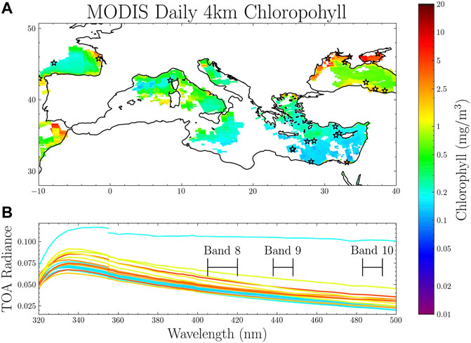
FIGURE 1. Satellite observations over the Mediterranean Sea from 15 March 2005. (A) MODIS daily 4 km chlorophyll concentration co-located to the OMI Fields of View (FoVs), stars correspond to radiances plotted in bottom; (B) cloud-free TOA radiances from OMI for several random locations plotted as a function of wavelength with the color representing the MODIS chlorophyll concentration. The lines on the plot represent the MODIS bands that are in OMI’s spectral range.

TROPOMI is a higher spatial resolution spectrometer launched in 2017 on the Sentinel-5P (S5P) polar orbiting satellite as a part of the Copernicus program of the European Commission (Veefkind et al., 2012). The S5P satellite was the first of the Copernicus missions dedicated to measuring trace gases and aerosols for air quality, climate, and ozone science. It is in a different orbit than Aura and Aqua but has a similar afternoon local equator crossing time at 13:30. The TROPOMI instrument has three CCDs that cover the wavelength range of 270–775 nm (UV, vis, and NIR) and one CCD that measures at longer wavelengths in the SWIR. It has a spectral resolution of 0.25–0.5 nm, which is similar to OMI, but the spatial resolution is much improved with a nadir spatial resolution of 5.5 × 3.5 km (prior to 6 August 2019, the spatial resolution was 7 × 3.5 km), which is closer to typical ocean color instruments. Here, we use TROPOMI bands 3 (320–405 nm) and 4 (405–500 nm) as there are geo-location differences between the UV-vis and NIR bands, making it difficult to use all the wavelengths from these bands simultaneously (Ludewig et al., 2020). The TROPOMI L1b processor was updated in July 2020 but at that time, the mission record before then had not been reprocessed. For this reason, we only used TROPOMI data after August 2020 in this study.

Unlike the SeaWiFS and MODIS instruments, future ocean color missions such as PACE will be hyperspectral and have higher spectral resolution. However, the spectral resolution of OMI and TROPOMI exceed that of PACE considerably. One of the goals of this study is to demonstrate that our approach will be effective if applied to PACE OCI measurements. We, therefore, have convolved UV and vis sun-normalized TOA radiances from OMI and TROPOMI used in this study with a triangular function of 2.5 nm FWHM sampled every 2.5 nm, which is similar to the PACE FWHM of 5 nm and spacing of 2.5 nm. For OMI, we use TOA radiances every 2.5 nm from 320–500 nm (74 wavelengths total) including those in the overlap between UV-2 and vis channels near 355 nm. The measurements in the overlap region between TROPOMI channels have greater noise as well, so only TROPOMI data between 320–400 nm and 405–497.5 nm (70 wavelengths total) are used. We note that we do not use the PACE noise, which could degrade our results. In the supplement, the RMSE of R_rs and chlorophyll shows little to no change when using the nominal high spectral resolution measurements from OMI. However, when smoothing to the PACE FWHM of 5 nm, the 443 nm R_rs RMSE increases from 8.21e-4 to 8.88e-4 and log (CHL) RMSE increases from 0.101 to 0.102.

Figure 1 shows an example of OMI-smoothed measured radiances for a few random locations across the Mediterranean Sea on 25 March 2005. In the top panel, the MODIS-retrieved chlorophyll concentration is mapped on the OMI FoV with the stars denoting the locations of the spectra that are plotted in the bottom panel and color coded based on the retrieved MODIS chlorophyll concentration. In this figure, similar chlorophyll concentration measurements have very different UV–vis measured spectra indicating that the atmospheric signal is much larger than the signal from the ocean surface.

2.2 MODIS Ocean Color Data

Ocean color retrievals of chlorophyll concentration and R_rs at 412 nm, 443 nm, and 488 nm from the Aqua MODIS instrument (Franz et al., 2005) are used to train the neural network. The MODIS R_rs data are normalized for bi-directional reflectance (BRDF) effects, but we note that any error in this BRDF normalization could lead to an error in the approach (Mobley et al., 2016). Since OMI and TROPOMI measurements have lower spatial resolution than MODIS, 4 km ocean color products from MODIS are averaged over the OMI and TROPOMI FoV. This collocation allows us to train the neural network to retrieve ocean color properties under cloud, aerosol, and sunglint conditions as a portion of the coarser OMI and TROPOMI FoVs contains these effects. If less than 50% of valid coverage from the daily Aqua MODIS product is available for an OMI or TROPOMI FoV, it is gap-filled using the MODIS 8-day composite to provide more full global coverage under cloud, aerosol and sunglint conditions. If neither the daily or 8-day MODIS retrievals can provide 50% coverage in the OMI or TROPOMI FoV, that pixel is not considered.

There is another MODIS instrument onboard NASA’s Terra satellite which has a morning overpass time. Terra is in a different orbit than Aura or Aqua so we do not include the data from the MODIS Terra instrument in the training. However, we do show ocean color retrievals from MODIS Terra in the validation to show the daily coverage of ocean color available from both MODIS instruments.

We do note that there are some accuracy issues with the MODIS ocean color retrievals being used in this work. As discussed in the work by Franz et al. (2012), absorbing aerosols are not easy to distinguish from non-absorbing aerosols; thus, the impact of absorbing aerosols is not included in the MODIS atmospheric correction. Also, the work by Chaves et al. (2015) showed that the MODIS chlorophyll concentration is biased particularly at higher latitudes due to the effects of absorption of colored dissolved organic matter on R_rs. In addition, it has been shown that the MODIS ocean color properties have large uncertainty at higher solar angles due to effects such as BRDF (particularly for low chlorophyll concentrations) and uncertainties about phytoplankton absorption properties at high latitudes (Suzuki et al., 1998; Li et al., 2017, 2019). We note that these biases and uncertainties in the MODIS retrievals would likely carry over to our results from OMI and TROPOMI, and as a neural network estimate can only be as good as the data that were used in the training.

2.3 SeaBASS Ocean Color Data

Through independent validation of our results, we compare the neural network (NN)-derived chlorophyll concentration and R_rs from OMI with in situ measurements from various field campaigns available in NASA’s SeaWiFS Bio-optical Archive and Storage System (SeaBASS). Given that OMI only measures to 500 nm, we compare with in situ R_rs at 412, 443, and 488 nm. The validation data available from the SeaBASS webpage are co-located to MODIS and are the best match-ups for validating MODIS (Bailey and Werdell, 2006). These data are from different campaigns and cover different oceanic and coastal regions. There are no in situ measurements available in this dataset during the TROPOMI record; thus, in situ comparisons are only done for OMI.

As per the recommendations by EUMETSAT (2019), we only use OMI scenes where the solar zenith angles are less than 60° and view zenith angle is less than 70°. While it is recommended to use multiple pixels from the satellite measurements in the in situ comparison, the OMI FoV is significantly larger than instruments such as MODIS that are typically used; thus, we instead compare individual OMI pixels with the in situ measurements. Any OMI scenes that satisfy the solar and view zenith angle conditions and are within 10 km of the in situ measurements are used in the comparison. Several statistics are used in this comparison including the root mean square error (RMSE), R², and bias as defined by Brewin et al. (2015).

2.4 Pre-Processing of Inputs

A key part in the development of a machine learning model is to use only the highest quality and most representative data in the training. For this reason, we apply several quality control steps before performing the training of our ocean color neural network.

Since the spectral dependence of land surface reflectance is quite different from that of water surface reflectance, we ignore pixels with mixed land and water. For OMI, only pixels with greater than 90% coverage of water are used in the training. However, TROPOMI only has a binary land water flag available, so the training is simply done wherever that flag is set to water. The TROPOMI L1b data also provide a land classification flag that is used to remove any pixels considered to be water mixed with land or coastline. We also do not use pixels classified as shallow inland water as the focus of this work is mainly on open ocean water and deep inland lakes.

While the main focus of this study is to reproduce ocean properties under clear and cloudy conditions, there are some optically thick clouds for which this approach does not work, so we used an effective cloud fraction (ECF) to remove optically thick clouds. Unlike more commonly used geometric cloud fractions, the ECF is radiometrically based so that it better represents not only the two-dimensional spatial distribution of clouds but also the optical depth of the cloud. Stammes et al. (2008) showed that an ECF of 0.5 corresponds to a cloud optical thickness of approximately 10. Scenes with ECF $>$ 0.5 are excluded from this study (25% of OMI scenes and 28% of TROPOMI scenes were excluded due to optically thick clouds). In addition, we exclude any data with a UV aerosol index (AI) greater than three as this indicates the presence of optically thick absorbing aerosols (0.06% of OMI scenes and 0.05% of TROPOMI scenes were excluded due to heavy aerosol loading) (Torres et al., 2013; Torres et al., 2020).

Ocean color retrievals are not performed over snow or ice so these data are removed based on co-located snow and ice flags using the National Snow and Ice Data Centers (NSIDC) Interactive Multisensor Snow and Ice Mapping System (IMS) in the northern hemisphere and the Near-real-time Ice and Snow Extent (NISE) data in the southern hemisphere (Brodzik and Stewart, 2016; U.S. National Ice Center, 2008). In addition, we ignore data below 70S as an extra measure for possible sea ice in case it is missed by the NISE flags.

2.5 Principal Component Analysis and Machine Learning Approach

A principal component analysis is performed on the measured hyperspectral radiances to extract empirical orthogonal functions (EOFs) in the form of a covariance matrix. The measured radiances are not corrected for any Rayleigh scattering or gas absorption as we assume that the principal component analysis can concentrate the relevant information content from the spectra and the neural network will learn to minimally weigh the information related to atmospheric absorption or scattering. The principal component analysis was performed for all OMI or TROPOMI samples that had available daily or 8-day composite co-located data from MODIS. For OMI, the principal component analysis is performed using 2 days from each month (1^st and 15^th) in 2005 with March being excluded so that it can be used to validate the technique. The TROPOMI principal component analysis is again based on 2 days a month from August–December 2020 with October excluded for validation. We note that for TROPOMI, we do not use the full year as the TROPOMI data were reprocessed with a new L1b processor beginning August 2020 but data from earlier in the mission have not yet been reprocessed. Figure 2 shows some of the principal components of the EOF decomposed from OMI-measured radiances. The leading principal component captures broad features due to Rayleigh scattering. Other leading principal components such as PC 4 and PC 5 appear to have information about other absorbers such as NO₂ and chlorophyll. The sharp discontinuity observed in several PCs at 355 nm is due to the disagreement between the OMI UV and vis channels. Lesser important PCs that account for less than 0.03% of the total variance seem to provide information on the instrumental effects.

FIGURE 2

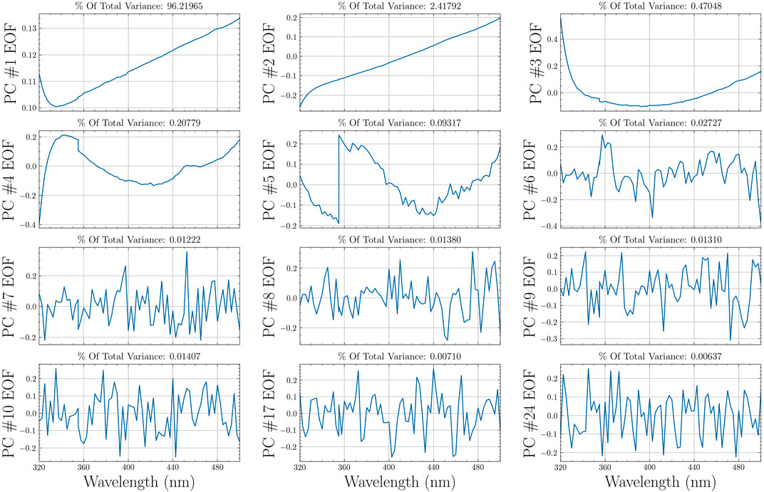
FIGURE 2. Orthogonal functions decomposed from OMI measurements from 2 days each month in 2005 (excluding March). The leading 10 EOFs are shown as well as lower ranked EOFs 17 and 24.

The leading eigenmodes of the covariance matrix can provide coefficients such that the linear combination of the PCs recreates the measured spectra. If the inputs to the principal component analysis are representative of most typical conditions, the principal components can be applied to extract coefficients from other spectra. Figure 3A shows an example of the coefficients of the principal components decomposed from OMI radiances on 15 March 2005, which was not included in the principal component decomposition performed on the training dataset. It shows that the amplitude of PC 1 is strongly correlated with the observed features in the OMI 400 nm TOA reflectance shown in Figure 3B. While the first few PCs provide information about the atmosphere, Figures 3C,D show that coefficients of the fourth PC are correlated with chlorophyll concentration.

FIGURE 3

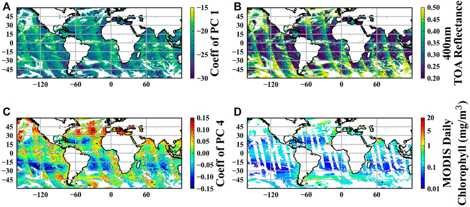
FIGURE 3. OMI measurements and MODIS ocean color retrievals for 15 March 2005. (A) Coefficient of the first PC; (B) 400 nm OMI-measured TOA reflectance; (C) coefficient of the fourth PC; (D) MODIS chlorophyll concentration co-located to OMI.

Once the coefficients of the PCs are extracted from the measured radiances, a neural network is trained to predict the ocean color properties for OMI/TROPOMI pixels that are co-located with the MODIS retrievals of R_rs and chlorophyll. Given the relatively coarse spatial resolution of OMI/TROPOMI measurements, there will be subgrid clouds in many of the co-located data points. Thus, the NN training is effectively confronted both with clear and cloudy observations. The PCA is able to transform the information from the measured spectra and provide it to the neural network in a way that makes it easier for the neural network to learn. The PC coefficients based on the satellite measured radiances are the inputs to the neural network, and the collocated MODIS-retrieved chlorophyll concentration and R_rs are the targets. A single neural network is used to reproduce chlorophyll concentration and R_rs. For this work, only the coefficients of the leading 30 PCs are used as inputs to the neural network, which account for 99.69% of the variance in the training data and 99.73% of the variance in the test data (further discussed in the Supplementary Material). In addition to using the coefficients of the principal components as inputs to the NN, the solar zenith, view zenith, and relative azimuth angles are also provided as inputs to the neural network to account for any dependence on view or solar geometry. In this approach, we assume that through the principal components, the neural network learns how to normalize for the BRDF effects in the OMI and TROPOMI measurements (Supplementary Material S1). We also include the across-track position in the training to help the NN learn about possible striping effects. As shown in Figure 4, the neural network used is a simple six-layer network (one input layer, four hidden layers, and one output layer) that uses the sigmoid activation function. The neural network was trained for 500 iterations and each of the four hidden layers has 32 nodes. The inputs and outputs are all scaled to the range of 0–1 for the training. When training the neural network, we use a random 50% of the samples that were used in the principal component analysis. The histograms in Figure 5 show the different conditions that are included in the training of the TROPOMI NN. This figure shows that a majority of the scenes include at least some partial clouds. In addition, approximately 40% of the input data potentially include sunglint-contaminated scenes as a glint angle less than 40° is generally used to classify potential sunglint-affected retrievals (Gupta et al., 2019).

FIGURE 4

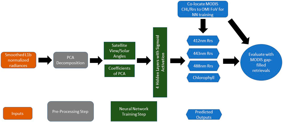
FIGURE 4. Flowchart showing how hyperspectral TOA radiances from OMI and TROPOMI are used to train a neural network to predict ocean color information using ocean color data from MODIS as the training dataset. A single neural network is used to predict all four outputs (details discussed in text).

FIGURE 5

FIGURE 5. Cumulative histograms of the conditions that are included in the input data to the TROPOMI NN training. (A) shows the ECF for the input data and (B) shows the glint angle of the NN training inputs.

3 Results

3.1 TROPOMI Ocean Color

Here, we present a case study of the approach applied to TROPOMI for 15 October 2020. The TROPOMI data from October 2020 were excluded from the PCA and neural network training so that it could be used for validation. Figure 6 shows a comparison of chlorophyll between the TROPOMI machine learning–based chlorophyll and the MODIS standard retrieval for 15 October 2020. There is generally good agreement between the TROPOMI chlorophyll and MODIS chlorophyll with a MAE of 0.09 and RMSE of 0.148 when comparing with daily MODIS Chl. The disagreement seems worse for the higher chlorophyll concentrations possibly due to the limited amount of high chlorophyll available in the training. The TROPOMI comparison to both the daily and 8-day MODIS retrievals is similar, suggesting that using the 8-day composite for gap filling works well for training the neural network where clouds, aerosols, or sunglint conditions exist. Similar comparisons are shown in Figure 7 for R_rs at 412, 443, and 488 nm. TROPOMI and MODIS are in excellent agreement at 412 and 443 nm with an R² of 0.910–0.926. The comparison is a little worse at 488 nm possibly because it is near the edge of the TROPOMI vis detector.

FIGURE 6

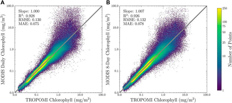
FIGURE 6. Comparisons of chlorophyll from the TROPOMI NN-based method and MODIS atmospheric correction-based retrieval for 15 October 2020. Statistics are shown for Log₁₀ of Chl. (A) Comparisons of TROPOMI NN-based chlorophyll with MODIS daily chlorophyll co-located to the TROPOMI FoV, (B) same as left but comparing with MODIS 8-day composite chlorophyll retrievals co-located to TROPOMI FoV.

FIGURE 7

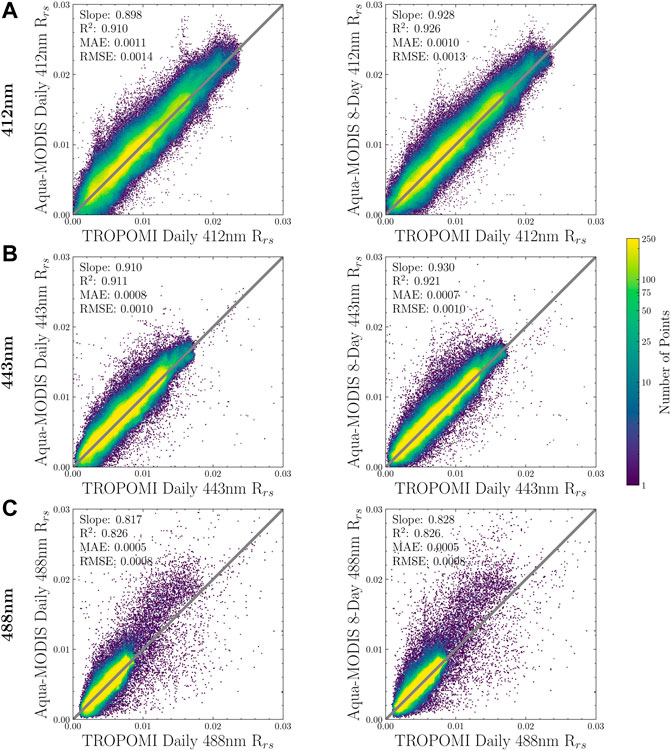
FIGURE 7. Same as Figure 6 but for comparisons of R_rs. (A) shows 412 nm R_rs, (B) shows 443 nm R_rs, and (C) shows 488 nm R_rs.

Since the aim of this research is to retrieve ocean color properties in cloud, aerosol, and sunglint conditions, we present Figure 8, which shows a comparison of the TROPOMI and MODIS R_rs retrievals for 20 October 2020 as a function of these variables. These plots were created using MODIS 8-day composite retrievals so that there would be MODIS data to compare with under cloud, aerosol, and sunglint conditions. The mean error in the TROPOMI machine learning–based chlorophyll grows above an ECF of 0.8 because there is a very low sensitivity to the surface. The middle panel of Figure 8 shows the difference between TROPOMI and MODIS R_rs as a function of glint angle with sunglint generally having glint angles of less than 20°. There is no significant dependence of the error on glint angle, suggesting that this method is working even for sunglint conditions. Finally, there is some dependence on AI with error increasing for AI $<$ -2 and AI $>$ 1, but we also note that the AI from TROPOMI is centered around -1.75. This suggests that the approach could work well for even moderate absorbing aerosol loading scenes.

FIGURE 8

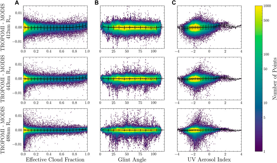
FIGURE 8. Difference on 15 October 2020 between TROPOMI and MODIS Rrs at 412 nm (top), 443 nm (middle), and 488 nm (bottom) as a function of ECF (A), glint angle (B), and aerosol index (C). The black line represents the mean error with the error bars showing +/− 1 standard deviation. The data in this figure were not screened for clouds, aerosols, or sunglint.

Figure 9 shows how the difference between TROPOMI and MODIS R_rs changes compared with the 412 nm measured TOA reflectance from TROPOMI. For TOA reflectance $<$ 0.7, the MODIS R_rs is about 0.001 higher than TROPOMI at 412 and 443 nm, while at 488 nm, the mean difference is almost 0. The mean difference increases to 0.002 for TOA reflectance $>$ 0.7, which is likely due to increased cloudiness in the TROPOMI FoV that limits the signal from the surface. This suggests that the technique is limited for TOA reflectance at 412 nm greater than 0.7.

FIGURE 9

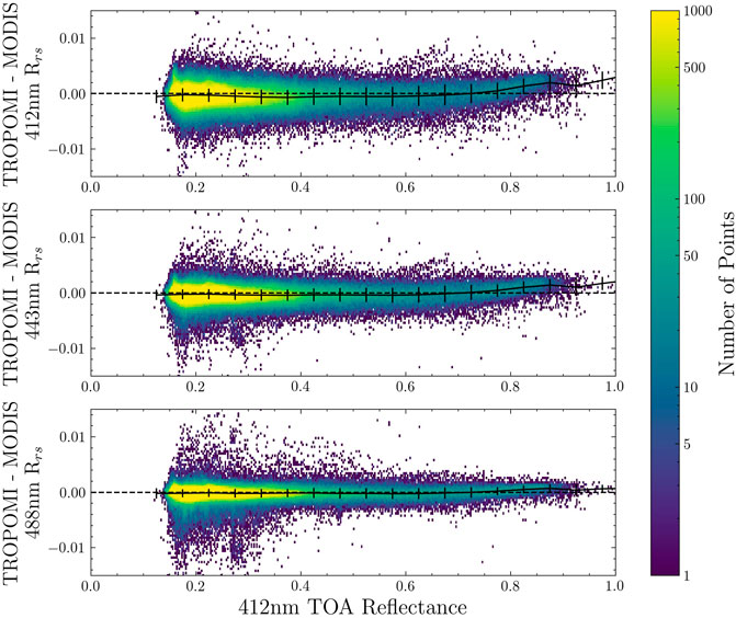
FIGURE 9. Difference on 15 October 2020 between TROPOMI and MODIS Rrs at 412 nm (top), 443 nm (middle), and 488 nm (bottom) as a function of 412 nm TOA reflectance. The black line represents the mean error with the error bars showing +/− 1 standard deviation. The data in this figure were not screened for clouds, aerosols, or sunglint.

In Figure 10, the TROPOMI machine learning–based chlorophyll and MODIS-retrieved chlorophyll are mapped for 15 October 2020 at a spatial resolution of 4 km. We include chlorophyll retrievals from both the Aqua-MODIS and Terra-MODIS instruments in the MODIS daily chlorophyll concentration map to show the total possible coverage available from MODIS on a daily basis. The differences in chlorophyll between TROPOMI and MODIS are generally less than 25%, with some larger differences particularly in higher latitude regions. The TROPOMI daily chlorophyll has coverage for about 47% of the global ocean while the MODIS daily chlorophyll and MODIS Aqua 8-day composite only have 16 and 42% coverage, respectively. For example, the TROPOMI chlorophyll is elevated just off the western coast of Saharan Africa, but this region is missing in both the MODIS daily and 8-day composite images. This is true for several coastal regions globally since the TROPOMI neural network algorithm is able to retrieve under partial clouds. This suggests that the machine learning approach would have better ability to monitor global chlorophyll and HABs in near real-time. In addition, there is no noticeable degradation or discontinuities in the sunglint region from the TROPOMI chlorophyll in Figure 10, whereas the MODIS daily chlorophyll retrieval has a large area missing in each orbit due to sunglint conditions. Supplementary Figures S2–S5 show analogous comparisons of OMI neural network retrievals to MODIS on 15 March 2005 with comparable results as shown with TROPOMI.

FIGURE 10

FIGURE 10. Retrievals of chlorophyll for 15 October 2020 gridded to 4 km. (A) TROPOMI machine learning–based chlorophyll; (B) Aqua MODIS daily chlorophyll retrieval gap-filled with the Terra-MODIS daily chlorophyll retrieval; (C) Aqua-MODIS 8-day chlorophyll retrieval; (D) percent difference between the TROPOMI machine learning–based chlorophyll and the Aqua MODIS daily chlorophyll gap filled with Terra MODIS.

Next, we will show comparisons of TROPOMI and MODIS chlorophyll retrievals over specific regions. Figure 11 shows a case study in the Gulf of Mexico on 10 October 2020, which had considerable cloudiness. While the MODIS daily chlorophyll retrievals are quite limited on this day, the TROPOMI machine learning approach has very few gaps in coverage on this day. The general patterns in the TROPOMI NN-based chlorophyll compare well with the MODIS-Aqua daily chlorophyll where available. In the central Gulf of Mexico, both the TROPOMI chlorophyll and MODIS daily chlorophyll appear higher than in the MODIS 8-day composite as it seems the 8-day composite likely smoothens a lot of the dynamic gyre-like features. In addition, there is no noticeable contamination in the TROPOMI chlorophyll from sunglint features.

FIGURE 11

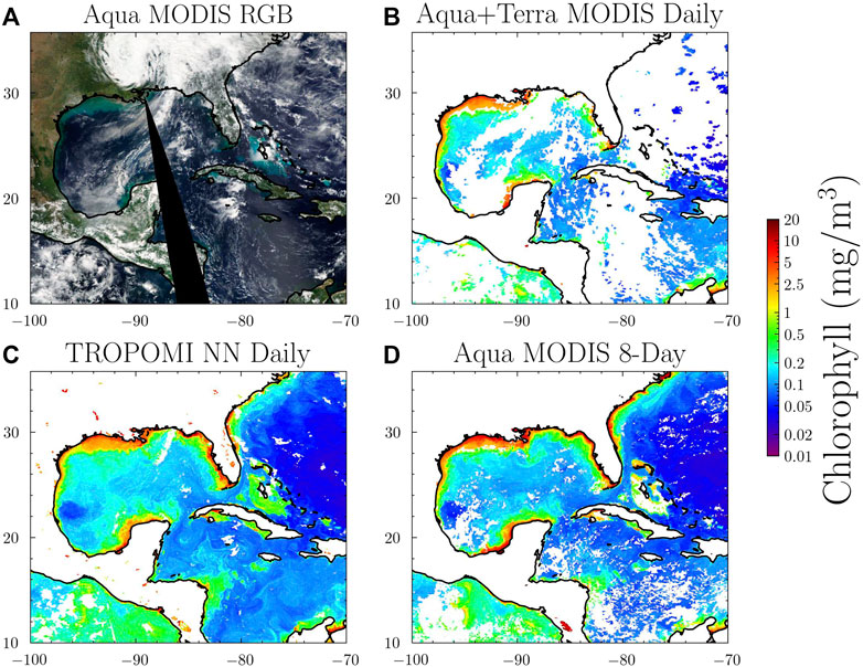
FIGURE 11. Chlorophyll retrievals in the Gulf of Mexico for 10 October 2020. (A) shows a true color image from MODIS Aqua, (B) shows MODIS-Aqua daily 4 km retrieval, (C) shows TROPOMI machine learning–based chlorophyll, and (D) shows MODIS-Aqua 8-day composite of chlorophyll.

In Figure 12, we show the results for a final case study of the TROPOMI chlorophyll in the Arabian Sea on 13 October 2020. There is considerable cloudiness across much of the Arabian Sea significantly limiting the spatial coverage from the MODIS daily chlorophyll. The TROPOMI machine learning–based chlorophyll, however, provides nearly full spatial coverage across the Arabian Sea and captures many of the chlorophyll features in the region. While the MODIS Aqua 8-day chlorophyll composite has better spatial coverage than the daily MODIS chlorophyll, it does not capture well the large gyre-like chlorophyll features in the central Arabian Sea. These gyre-like features can be seen well in the TROPOMI chlorophyll despite the clouds in the region.

FIGURE 12

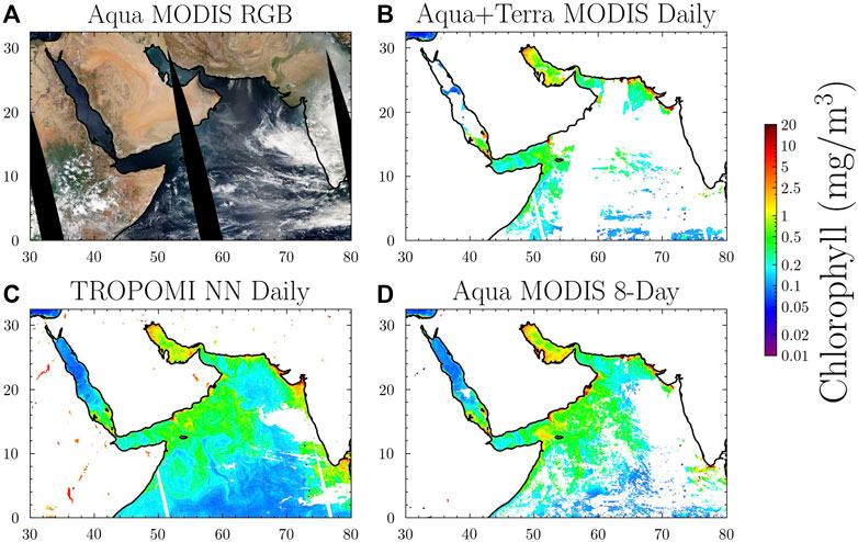
FIGURE 12. Chlorophyll retrievals in the Arabian Sea on 13 October 2020. (A) shows a true color image from MODIS Aqua, (B) shows MODIS-Aqua daily 4 km retrieval, (C) shows TROPOMI machine learning–based chlorophyll, and (D) shows MODIS-Aqua 8-day composite of chlorophyll.

Finally, in Figure 13, we present another example in northern Brazil near the mouth of the Amazon River. In this case, the MODIS daily chlorophyll is very limited due to a combination of sunglint and cloud cover across the region. While the Aqua MODIS 8-day composite has better coverage than the MODIS daily chlorophyll, it still has many gaps including at the outflow of the Amazon River, where there is a large region of elevated chlorophyll. The TROPOMI chlorophyll has much better coverage than both the MODIS daily chlorophyll and Aqua MODIS 8-day chlorophyll composite. The plumes of chlorophyll that extend into the ocean look nearly identical between the TROPOMI NN-based chlorophyll and the Aqua MODIS 8-day composite chlorophyll. The structure of the elevated chlorophyll along the coast in the TROPOMI looks very similar to that of the Aqua MODIS 8-day chlorophyll composite but slightly lower. It is worth noting that the coastal waters in the region may also include suspended particles and elevated CDOM concentrations, which could also impact the measured TOA radiance. In the open ocean, the TROPOMI chlorophyll has much more complete coverage than the MODIS daily chlorophyll and Aqua MODIS 8-day composite chlorophyll.

FIGURE 13

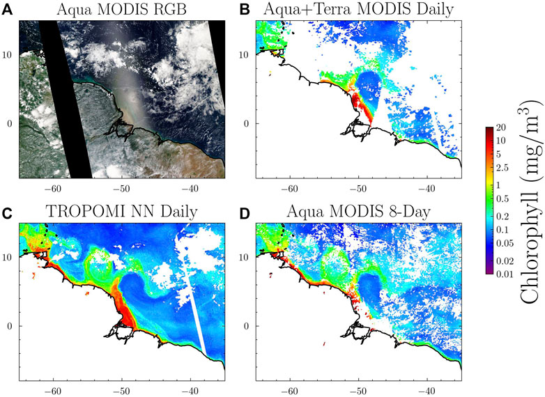
FIGURE 13. Chlorophyll retrievals for the coast of northern Brazil on 10 October 2020. (A) shows true color image from MODIS Aqua, (B) shows MODIS-Aqua daily 4 km retrieval, bottom (C) TROPOMI machine learning–based chlorophyll, and (D) shows MODIS-Aqua 8-day composite of chlorophyll.

3.2 OMI In Situ Comparison

To further evaluate the machine learning–based approach, we compare the machine learning–based chlorophyll with in situ measurements from SeaBASS in Figures 14, 15. As previously noted, this comparison is done with OMI as there is limited in situ data available during the TROPOMI mission. Here, we include comparisons of in situ data with OMI machine learning approach (left panel), MODIS at its native resolution (middle panel), and MODIS co-located to the OMI FoV (right panel) in order to examine the impact of OMI’s coarser spatial resolution in the validation. Optically thick clouds (ECF $>$ 0.5) and heavy aerosol loading scenes ($|AI|>$ 3) were excluded, but ultimately, we found there were no such cases for the in situ validation data anyway. The in situ comparisons of chlorophyll are quite similar for both OMI and MODIS, which is expected since the OMI NN is trained for retrievals from MODIS. The OMI machine learning–based chlorophyll had an RMSE of 2.38 while MODIS chlorophyll on the OMI FoV had an RMSE of 2.43. This is not the case in the R_rs retrievals shown in Figure 15; however, the MODIS R_rs retrievals at the native resolution compared better with the in situ measurements than those on the OMI FoV. The OMI machine learning–based R_rs comparison to in situ data is a little worse than the MODIS comparisons with the in situ data.

FIGURE 14

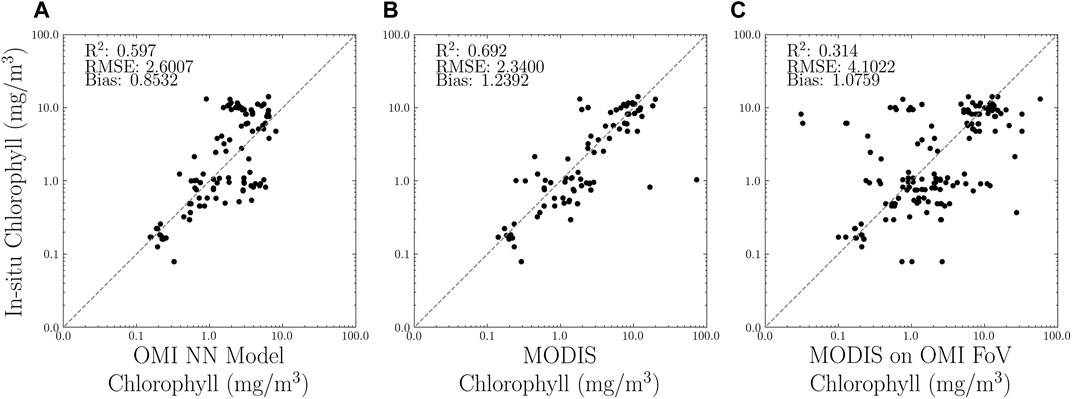
FIGURE 14. Retrievals of chlorophyll compared with in situ measurements. (A) is the OMI machine learning–based chlorophyll, (B) is the MODIS-Aqua chlorophyll at the native resolution, and (C) is the MODIS-Aqua chlorophyll retrieval co-located to the OMI FoV. There are 163 co-located points in the comparison.

FIGURE 15

FIGURE 15. Similar to Figure 14 but for R_rs. (A) are for 412 nm, (B) are 443 nm, and (C) are 488 nm. There are 340 co-located points in the comparison.

4 Conclusion

We have proposed a method for filling in the gaps of multi-spectral satellite ocean color retrievals from instruments such as MODIS when clouds, aerosols, and sunglint interfere with traditional methods. We demonstrated our approach using hyperspectral data from the OMI and TROPOMI instruments, which have lower spatial resolution but serve as a useful proxy for PACE OCI measurements. Our approach is based on performing a principal component analysis on hyperspectral radiances to extract spectral features and then training a neural network to predict MODIS standard ocean color retrieval data from the coefficients of the leading PCs of OMI and TROPOMI radiances. We used daily MODIS ocean color retrievals and MODIS 8-day ocean color composites collocated to OMI and TROPOMI observations to provide training data to the neural network globally, which provided a variety of conditions such as clouds, aerosols, and sunglint contamination for training.

The approach has been applied to spectrally smoothed OMI and TROPOMI high spectral resolution measurements from 320–500 nm. Results from this approach compare well with the standard retrievals from MODIS that utilize atmospheric correction. In addition, the method on the coarse OMI and TROPOMI pixels shows little degradation compared to daily and 8-day MODIS composites, suggesting that the approach performs well for clouds, aerosols, and sunglint, which are less-than-ideal conditions for standard multi-spectral ocean color retrievals. Comparisons between the OMI ocean color estimates and in situ measurements show very similar results with MODIS, suggesting that the approach has similar accuracy to the traditional MODIS retrievals. We do note, however, for heavy absorbing aerosol loading and optically thick clouds, the approach does not work quite as well.

Even though the approach is shown to be promising for OMI and TROPOMI, there are some uncertainties that could provide areas for future improvements. In this work, aerosol index based on UV wavelengths was used to remove potentially heavy aerosol loading scenes. It is known that there are some uncertainties in separating the aerosol signal from the ocean color signal; thus, improved aerosol information could help to improve the selection of input data for the PCA and NN (Torres et al., 2013). It can be assumed that the BRDF effects are different for MODIS and OMI or TROPOMI, and while principal component analysis and neural network may learn how to correct for some of these BRDF effects, there likely is still error due to these effects. It would be beneficial to use training data from the same satellite the approach is being applied to in order to avoid such errors due to BRDF differences between two instruments. This will be possible with some of the future ocean color instruments such as PACE that will provide much higher spectral resolution than the heritage ocean color missions. In addition, many of the upcoming hyperspectral missions will have measurements through the red band, which could provide additional spectral information that could improve the atmospheric correction. In future works, this will be tested using TROPOMI, assuming the geo-location mismatch between the TROPOMI bands can be corrected. Future works will also further evaluate the performance of this approach for case 1 and case 2 waters.

Since OMI has been in flight for over 17 years, the development of an ocean color product from OMI could provide useful information by increasing global daily coverage of ocean color retrievals. While it would not provide the high resolution information available from MODIS, it could be beneficial in frequently overcast regions where MODIS-based retrievals are limited. In addition, TROPOMI could be used to gap fill MODIS retrievals starting in 2018 and provide measurements of ocean color properties that are only slightly coarser resolution than MODIS.

This approach also provides a method for near real-time monitoring of ocean color properties such as chlorophyll. Over the next few years, there will be several new hyperspectral instruments launched for which this approach could be applied. In 2022, NASA’s geostationary Tropospheric Emissions: Monitoring of Pollution (TEMPO) will launch taking measurements across North America hourly with a 5 km spatial resolution (Zoogman et al., 2017). TEMPO will provide a unique opportunity to capture the diurnal changes in the ocean biology of coastal regions including the Gulf of Mexico and the Pacific and Atlantic coasts. The OCI instrument onboard PACE will launch in 2024 as the first hyperspectral instrument dedicated to ocean measurements. Given enough overlap with a well-calibrated L2 ocean color product from an instrument such as MODIS, VIIRS, or OCLI, it may be possible to use this approach to produce an early mission product even with an imperfect L1 calibration. In future works, we will examine whether such an approach is possible with early mission L1 calibration. Both of these instruments will take measurements from the UV through the red edge to allow for possible improvements of this method with the increased spectral information. This approach will also be applicable to NASA’s Geosynchronous Littoral Imaging and Monitoring Radiometer (GLIMR) instrument, which will launch in 2026–2027 taking hourly hyperspectral measurements in the Gulf of Mexico, southern U.S. coastline, and tropical Atlantic Ocean.

Data Availability Statement

The raw data supporting the conclusion of this article will be made available by the authors, without undue reservation.

Author Contributions

ZF was responsible for applying the methodology, data curation, visualization, formal analysis, and wrote the first draft. JJ developed the method and contributed to the manuscript preparation. NK acquired the funding and contributed to the manuscript preparation. DH, WQ, AV, and PC contributed to the manuscript preparation.

Funding

This work was supported by NASA’s Earth Science Division through its Earth Observing System Aura project and the OMI (NNH19ZDA001N-AURAST) and PACE (NNH19ZDA001N-PACESAT) science teams.

Conflict of Interest

ZF, DH, WQ, and AV were employed by Science Systems and Applications, Inc.

The remaining authors declare that the research was conducted in the absence of any commercial or financial relationships that could be construed as a potential conflict of interest.

Publisher’s Note

All claims expressed in this article are solely those of the authors and do not necessarily represent those of their affiliated organizations, or those of the publisher, the editors, and the reviewers. Any product that may be evaluated in this article, or claim that may be made by its manufacturer, is not guaranteed or endorsed by the publisher.

Acknowledgments

We are grateful to the NASA’s Ocean Biology Processing Group for providing the MODIS ocean color data. We thank those involved in the calibration of the instruments including the NASA OMI science team and TROPOMI science team. We also acknowledge the National Snow and Ice Data Center (NSIDC) for providing the snow and ice data.

Supplementary Material

The Supplementary Material for this article can be found online at: https://www.frontiersin.org/articles/10.3389/frsen.2022.846174/full#supplementary-material

References

Bailey, S. W., and Werdell, P. J. (2006). A Multi-Sensor Approach for the On-Orbit Validation of Ocean Color Satellite Data Products. Remote Sensing Environ. 102, 12–23. doi:10.1016/j.rse.2006.01.015

CrossRef Full Text | Google Scholar

Bracher, A., Vountas, M., Dinter, T., Burrows, J. P., Röttgers, R., and Peeken, I. (2009). Quantitative Observation of Cyanobacteria and Diatoms from Space Using Phytodoas on Sciamachy Data. Biogeosciences 6, 751–764. doi:10.5194/bg-6-751-2009

CrossRef Full Text | Google Scholar

Brewin, R. J. W., Sathyendranath, S., Müller, D., Brockmann, C., Deschamps, P.-Y., Devred, E., et al. (2015). The Ocean Colour Climate Change Initiative: Iii. A Round-Robin Comparison on In-Water Bio-Optical Algorithms. Remote Sensing Environ. 162, 271–294. doi:10.1016/j.rse.2013.09.016

CrossRef Full Text | Google Scholar

[Dataset] Brodzik, M. J., and Stewart, J. S. (2016). Near-real-time Ssm/i-Ssmis Ease-Grid Daily Global Ice Concentration and Snow Extent, Version 5. doi:10.5067/3KB2JPLFPK3R

CrossRef Full Text | Google Scholar

Chaves, J. E., Werdell, P. J., Proctor, C. W., Neeley, A. R., Freeman, S. A., Thomas, C. S., et al. (2015). Assessment of Ocean Color Data Records from Modis-Aqua in the Western Arctic Ocean. Deep Sea Res. Part Topical Stud. Oceanography 118, 32–43. doi:10.1016/j.dsr2.2015.02.011

CrossRef Full Text | Google Scholar

Chen, S., Hu, C., Barnes, B. B., Xie, Y., Lin, G., and Qiu, Z. (2019). Improving Ocean Color Data Coverage through Machine Learning. Remote sensing Environ. 222, 286–302. doi:10.1016/j.rse.2018.12.023

CrossRef Full Text | Google Scholar

Dierssen, H. M. (2010). Perspectives on Empirical Approaches for Ocean Color Remote Sensing of Chlorophyll in a Changing Climate. Proc. Natl. Acad. Sci. U.S.A. 107, 17073–17078. doi:10.1073/pnas.0913800107

PubMed Abstract | CrossRef Full Text | Google Scholar

Dinter, T., Rozanov, V. V., Burrows, J. P., and Bracher, A. (2015). Retrieving the Availability of Light in the Ocean Utilising Spectral Signatures of Vibrational Raman Scattering in Hyper-Spectral Satellite Measurements. Ocean Sci. 11, 373–389. doi:10.5194/os-11-373-2015

CrossRef Full Text | Google Scholar

EUMETSAT (2019). Recommendations for sentinel-3 Olci Ocean Colour Product Validations in Comparison with in Situ Measurements. Darmstadt, Germany: EUMETSAT.

Google Scholar

Evans, R. H., and Gordon, H. R. (1994). Coastal Zone Color Scanner “System Calibration”: A Retrospective Examination. J. Geophys. Res. 99, 7293–7307. doi:10.1029/93jc02151

CrossRef Full Text | Google Scholar

Franz, B. A., Bailey, S. W., Meister, G., and Werdell, P. J. (2012). Quality and Consistency of the Nasa Ocean Color Data Record. Proc. Ocean Opt. XXI.

Google Scholar

Franz, B. A., Bailey, S. W., Werdell, P. J., and McClain, C. R. (2007). Sensor-independent Approach to the Vicarious Calibration of Satellite Ocean Color Radiometry. Appl. Opt. 46, 5068–5082. doi:10.1364/ao.46.005068

PubMed Abstract | CrossRef Full Text | Google Scholar

Franz, B. A., Werdell, P. J., Meister, G., Bailey, S. W., Eplee, R. E., Feldman, G. C., et al. (2005). “The Continuity of Ocean Color Measurements from Seawifs to Modis,” in Earth Observing Systems X (Bellingham, Washington, USA: International Society for Optics and Photonics), Vol. 5882, 58820W. doi:10.1117/12.620069

CrossRef Full Text | Google Scholar

Frouin, R., Duforêt, L., and Steinmetz, F. (2014). “Atmospheric Correction of Satellite Ocean-Color Imagery in the Presence of Semi-transparent Clouds,” in Ocean Remote Sensing and Monitoring from Space (Bellingham, Washington, USA: International Society for Optics and Photonics), Vol. 9261, 926108. doi:10.1117/12.2074008

CrossRef Full Text | Google Scholar

Frouin, R. J., and Gross-Colzy, L. S. (2016). “Contribution of Ultraviolet and Shortwave Infrared Observations to Atmospheric Correction of Pace Ocean-Color Imagery,” in Remote Sensing of the Oceans and Inland Waters: Techniques, Applications, and Challenges (Bellingham, Washington, USA: International Society for Optics and Photonics), Vol. 9878, 98780C. doi:10.1117/12.2229891

CrossRef Full Text | Google Scholar

Gordon, H. R. (1997). Atmospheric Correction of Ocean Color Imagery in the Earth Observing System Era. J. Geophys. Res. 102, 17081–17106. doi:10.1029/96jd02443

CrossRef Full Text | Google Scholar

Gordon, H. R., and Wang, M. (1994). Retrieval of Water-Leaving Radiance and Aerosol Optical Thickness over the Oceans with Seawifs: a Preliminary Algorithm. Appl. Opt. 33, 443–452. doi:10.1364/ao.33.000443

PubMed Abstract | CrossRef Full Text | Google Scholar

Gross-Colzy, L., Colzy, S., Frouin, R., and Henry, P. (2007b). “A General Ocean Color Atmospheric Correction Scheme Based on Principal Components Analysis: Part Ii. Level 4 Merging Capabilities,” in Coastal Ocean Remote Sensing (Bellingham, Washington, USA: International Society for Optics and Photonics), Vol. 6680, 668003. doi:10.1117/12.738514

CrossRef Full Text | Google Scholar

Gross-Colzy, L., Colzy, S., Frouin, R., and Henry, P. (2007a). “A General Ocean Color Atmospheric Correction Scheme Based on Principal Components Analysis: Part I. Performance on Case 1 and Case 2 Waters,” in Coastal Ocean Remote Sensing (Bellingham, Washington, USA: International Society for Optics and Photonics), Vol. 6680, 668002. doi:10.1117/12.738508

CrossRef Full Text | Google Scholar

Gupta, P., Levy, R. C., Mattoo, S., Remer, L. A., Holz, R. E., and Heidinger, A. K. (2019). Applying the Dark Target Aerosol Algorithm with Advanced Himawari Imager Observations during the Korus-Aq Field Campaign. Atmos. Meas. Tech. 12, 6557–6577. doi:10.5194/amt-12-6557-2019

CrossRef Full Text | Google Scholar

Ioannou, I., Gilerson, A., Gross, B., Moshary, F., and Ahmed, S. (2011). Neural Network Approach to Retrieve the Inherent Optical Properties of the Ocean from Observations of Modis. Appl. Opt. 50, 3168–3186. doi:10.1364/ao.50.003168

PubMed Abstract | CrossRef Full Text | Google Scholar

Joiner, J., Fasnacht, Z., Gao, B.-C., and Qin, W. (2021a). Use of Hyper-Spectral Visible and Near-Infrared Satellite Data for Timely Estimates of the Earth's Surface Reflectance in Cloudy Conditions: Part 2- Image Restoration with HICO Satellite Data in Overcast Conditions. Front. Remote Sens. 2, 21. doi:10.3389/frsen.2021.721957

CrossRef Full Text | Google Scholar

Joiner, J., Fasnacht, Z., Qin, W., Yoshida, Y., Vasilkov, A., Li, C., et al. (2021b). Use of Multi-Spectral Visible and Near-Infrared Satellite Data for Timely Estimates of the Earth’s Surface Reflectance in Cloudy and Aerosol Loaded Conditions: Part 1-application to Rgb Image Restoration over Land with Gome-2. Submitted.

Google Scholar

Joiner, J., Yoshida, Y., Guanter, L., and Middleton, E. M. (2016). New Methods for the Retrieval of Chlorophyll Red Fluorescence from Hyperspectral Satellite Instruments: Simulations and Application to Gome-2 and Sciamachy. Atmos. Meas. Tech. 9, 3939–3967. doi:10.5194/amt-9-3939-2016

CrossRef Full Text | Google Scholar

Köhler, P., Behrenfeld, M. J., Landgraf, J., Joiner, J., Magney, T. S., and Frankenberg, C. (2020). Global Retrievals of Solar-Induced Chlorophyll Fluorescence at Red Wavelengths with Tropomi. Geophys. Res. Lett. 47, e2020GL087541.

CrossRef Full Text | Google Scholar

Levelt, P. F., Joiner, J., Tamminen, J., Veefkind, J. P., Bhartia, P. K., Stein Zweers, D. C., et al. (2018). The Ozone Monitoring Instrument: Overview of 14 Years in Space. Atmos. Chem. Phys. 18, 5699–5745. doi:10.5194/acp-18-5699-2018

CrossRef Full Text | Google Scholar

Levelt, P. F., Van Den Oord, G. H. J., Dobber, M. R., Malkki, A., Huib Visser, H., Johan de Vries, J., et al. (2006). The Ozone Monitoring Instrument. IEEE Trans. Geosci. Remote Sensing 44, 1093–1101. doi:10.1109/tgrs.2006.872333

CrossRef Full Text | Google Scholar

Li, H., He, X., Bai, Y., Chen, X., Gong, F., Zhu, Q., et al. (2017). Assessment of Satellite-Based Chlorophyll-A Retrieval Algorithms for High Solar Zenith Angle Conditions. J. Appl. Remote Sens 11, 012004. doi:10.1117/1.jrs.11.012004

CrossRef Full Text | Google Scholar

Li, H., He, X., Shanmugam, P., Bai, Y., Wang, D., Huang, H., et al. (2019). Radiometric Sensitivity and Signal Detectability of Ocean Color Satellite Sensor under High Solar Zenith Angles. IEEE Trans. Geosci. Remote Sensing 57, 8492–8505. doi:10.1109/TGRS.2019.2921341

CrossRef Full Text | Google Scholar

Ludewig, A., Kleipool, Q., Bartstra, R., Landzaat, R., Leloux, J., Loots, E., et al. (2020). In-flight Calibration Results of the Tropomi Payload on Board the sentinel-5 Precursor Satellite. Atmos. Meas. Tech. 13, 3561–3580. doi:10.5194/amt-13-3561-2020

CrossRef Full Text | Google Scholar

Millie, D. F., Schofield, O. M., Kirkpatrick, G. J., Johnsen, G., Tester, P. A., and Vinyard, B. T. (1997). Detection of Harmful Algal Blooms Using Photopigments and Absorption Signatures: A Case Study of the florida Red Tide Dinoflagellate, Gymnodinium Breve. Limnol. Oceanogr. 42, 1240–1251. doi:10.4319/lo.1997.42.5_part_2.1240

CrossRef Full Text | Google Scholar

Mobley, C. D., Werdell, J., Franz, B., Ahmad, Z., and Bailey, S. (2016). Tech. rep., National Aeronautics and Space Administration. Greenbelt, MD, USA: Goddard Space Flight Center.Atmospheric Correction for Satellite Ocean Color Radiometry

Google Scholar

Nieke, J., Borde, F., Mavrocordatos, C., Berruti, B., Delclaud, Y., Riti, J. B., et al. (2012). “The Ocean and Land Colour Imager (Olci) for the sentinel 3 Gmes mission: Status and First Test Results,” in Earth Observing Missions and Sensors: Development, Implementation, and Characterization II (Bellingham, Washington, USA: SPIE), Vol. 8528, 49–57. doi:10.1117/12.977247

CrossRef Full Text | Google Scholar

Oelker, J., Losa, S. N., Richter, A., and Bracher, A. (2022). Tropomi-retrieved Underwater Light Attenuation in Three Spectral Regions in the Ultraviolet and Blue. Front. Mar. Sci. 9. doi:10.3389/fmars.2022.787992

CrossRef Full Text | Google Scholar

Oelker, J., Richter, A., Dinter, T., Rozanov, V. V., Burrows, J. P., and Bracher, A. (2019). Global Diffuse Attenuation Derived from Vibrational Raman Scattering Detected in Hyperspectral Backscattered Satellite Spectra. Opt. Express 27, A829–A855. doi:10.1364/OE.27.00A829

PubMed Abstract | CrossRef Full Text | Google Scholar

O’Reilly, J. E., Maritorena, S., Mitchell, B. G., Siegel, D. A., Carder, K. L., Garver, S. A., et al. (1998). Ocean Color Chlorophyll Algorithms for Seawifs. J. Geophys. Res. Oceans 103, 24937–24953.

Google Scholar

Sadeghi, A., Dinter, T., Vountas, M., Taylor, B. B., Altenburg-Soppa, M., Peeken, I., et al. (2012). Improvement to the Phytodoas Method for Identification of Coccolithophores Using Hyper-Spectral Satellite Data. Ocean Sci. 8, 1055–1070. doi:10.5194/os-8-1055-2012

CrossRef Full Text | Google Scholar

Schenkeveld, V. M. E., Jaross, G., Marchenko, S., Haffner, D., Kleipool, Q. L., Rozemeijer, N. C., et al. (2017). In-flight Performance of the Ozone Monitoring Instrument. Atmos. Meas. Tech. 10, 1957–1986. doi:10.5194/amt-10-1957-2017

PubMed Abstract | CrossRef Full Text | Google Scholar

Schiller, H., and Doerffer, R. (1999). Neural Network for Emulation of an Inverse Model Operational Derivation of Case Ii Water Properties from Meris Data. Int. J. remote sensing 20, 1735–1746. doi:10.1080/014311699212443

CrossRef Full Text | Google Scholar

Sellner, K. G., Doucette, G. J., and Kirkpatrick, G. J. (2003). Harmful Algal Blooms: Causes, Impacts and Detection. J. Ind. Microbiol. Biotechnol. 30, 383–406. doi:10.1007/s10295-003-0074-9

PubMed Abstract | CrossRef Full Text | Google Scholar

Siegel, D. A., Maritorena, S., Nelson, N., Behrenfeld, M., and McClain, C. (2005). Colored Dissolved Organic Matter and its Influence on the Satellite-Based Characterization of the Ocean Biosphere. Geophys. Res. Lett. 32. doi:10.1029/2005gl024310

CrossRef Full Text | Google Scholar

Stammes, P., Sneep, M., De Haan, J., Veefkind, J., Wang, P., and Levelt, P. (2008). Effective Cloud Fractions from the Ozone Monitoring Instrument: Theoretical Framework and Validation. J. Geophys. Res. Atmospheres 113, 16. doi:10.1029/2007jd008820

CrossRef Full Text | Google Scholar

Steinmetz, F., Deschamps, P.-Y., and Ramon, D. (2011). Atmospheric Correction in Presence of Sun Glint: Application to Meris. Opt. Express 19, 9783–9800. doi:10.1364/oe.19.009783

PubMed Abstract | CrossRef Full Text | Google Scholar

Steinmetz, F., and Ramon, D. (2018). “Sentinel-2 Msi and sentinel-3 Olci Consistent Ocean Colour Products Using Polymer,” in Remote Sensing of the Open and Coastal Ocean and Inland Waters (Bellingham, Washington, USA: International Society for Optics and Photonics), Vol. 10778, 107780E. doi:10.1117/12.2500232

CrossRef Full Text | Google Scholar

Suzuki, K., Kishino, M., Sasaoka, K., Saitoh, S.-i., and Saino, T. (1998). Chlorophyll-specific Absorption Coefficients and Pigments of Phytoplankton off Sanriku, Northwestern north pacific. J. Oceanogr 54, 517–526. doi:10.1007/bf02742453

CrossRef Full Text | Google Scholar

Thome, K. J., Czapla-Myers, J. S., and Biggar, S. F. (2003). “Vicarious Calibration of Aqua and Terra Modis,” in Earth Observing Systems VIII (Bellingham, Washington, USA: SPIE), Vol. 5151, 395–405. doi:10.1117/12.506364

CrossRef Full Text | Google Scholar

Tilstone, G. H., Pardo, S., Dall'Olmo, G., Brewin, R. J. W., Nencioli, F., Dessailly, D., et al. (2021). Performance of Ocean Colour Chlorophyll a Algorithms for sentinel-3 Olci, Modis-Aqua and Suomi-Viirs in Open-Ocean Waters of the atlantic. Remote Sensing Environ. 260, 112444. doi:10.1016/j.rse.2021.112444

CrossRef Full Text | Google Scholar

Tjiputra, J. F., Polzin, D., and Winguth, A. M. (2007). Assimilation of Seasonal Chlorophyll and Nutrient Data into an Adjoint Three-Dimensional Ocean Carbon Cycle Model: Sensitivity Analysis and Ecosystem Parameter Optimization. Glob. Biogeochem. Cycles 21. doi:10.1029/2006gb002745

CrossRef Full Text | Google Scholar

Torres, O., Ahn, C., and Chen, Z. (2013). Improvements to the Omi Near-Uv Aerosol Algorithm Using A-Train Caliop and Airs Observations. Atmos. Meas. Tech. 6, 3257–3270. doi:10.5194/amt-6-3257-2013

CrossRef Full Text | Google Scholar

Torres, O., Jethva, H., Ahn, C., Jaross, G., and Loyola, D. G. (2020). TROPOMI Aerosol Products: Evaluation and Observations of Synoptic-Scale Carbonaceous Aerosol Plumes during 2018-2020. Atmos. Meas. Tech. 13, 6789–6806. doi:10.5194/amt-13-6789-2020

CrossRef Full Text | Google Scholar

[Dataset] U.S. National Ice Center (2008). Ims Daily Northern Hemisphere Snow and Ice Analysis at 1 Km, 4 Km, and 24 Km Resolutions, Version 1. doi:10.7265/N52R3PMC

CrossRef Full Text | Google Scholar

Veefkind, J. P., Aben, I., McMullan, K., Förster, H., De Vries, J., Otter, G., et al. (2012). Tropomi on the Esa sentinel-5 Precursor: A Gmes mission for Global Observations of the Atmospheric Composition for Climate, Air Quality and Ozone Layer Applications. Remote sensing Environ. 120, 70–83. doi:10.1016/j.rse.2011.09.027

CrossRef Full Text | Google Scholar

Vountas, M., Dinter, T., Bracher, A., Burrows, J. P., and Sierk, B. (2007). Spectral Studies of Ocean Water with Space-Borne Sensor Sciamachy Using Differential Optical Absorption Spectroscopy (Doas). Ocean Sci. 3, 429–440. doi:10.5194/os-3-429-2007

CrossRef Full Text | Google Scholar

Vountas, M., Richter, A., Wittrock, F., and Burrows, J. P. (2003). Inelastic Scattering in Ocean Water and its Impact on Trace Gas Retrievals from Satellite Data. Atmos. Chem. Phys. 3, 1365–1375. doi:10.5194/acp-3-1365-2003

CrossRef Full Text | Google Scholar

Wang, M., Liu, X., Jiang, L., Son, S., Sun, J., Shi, W., et al. (2014). “Evaluation of Viirs Ocean Color Products,” in Ocean Remote Sensing and Monitoring from Space (Bellingham, Washington, USA: International Society for Optics and Photonics), Vol. 9261, 92610E. doi:10.1117/12.2069251

CrossRef Full Text | Google Scholar

Wang, M., Liu, X., Tan, L., Jiang, L., Son, S., Shi, W., et al. (2013). Impacts of Viirs Sdr Performance on Ocean Color Products. J. Geophys. Res. Atmospheres 118, 10–347. doi:10.1002/jgrd.50793

CrossRef Full Text | Google Scholar

Werdell, P. J., McKinna, L. I. W., Boss, E., Ackleson, S. G., Craig, S. E., Gregg, W. W., et al. (2018). An Overview of Approaches and Challenges for Retrieving marine Inherent Optical Properties from Ocean Color Remote Sensing. Prog. oceanography 160, 186–212. doi:10.1016/j.pocean.2018.01.001

PubMed Abstract | CrossRef Full Text | Google Scholar

Wolanin, A., Rozanov, V. V., Dinter, T., Noël, S., Vountas, M., Burrows, J. P., et al. (2015). Global Retrieval of marine and Terrestrial Chlorophyll Fluorescence at its Red Peak Using Hyperspectral Top of Atmosphere Radiance Measurements: Feasibility Study and First Results. Remote Sensing Environ. 166, 243–261. doi:10.1016/j.rse.2015.05.018

CrossRef Full Text | Google Scholar

Zhang, M., Hu, C., and Barnes, B. B. (2019). Performance of Polymer Atmospheric Correction of Ocean Color Imagery in the Presence of Absorbing Aerosols. IEEE Trans. Geosci. Remote Sensing 57, 6666–6674. doi:10.1109/tgrs.2019.2907884

CrossRef Full Text | Google Scholar

Zoogman, P., Liu, X., Suleiman, R. M., Pennington, W. F., Flittner, D. E., Al-Saadi, J. A., et al. (2017). Tropospheric Emissions: Monitoring of Pollution (Tempo). J. Quantitative Spectrosc. Radiative Transfer 186, 17–39. doi:10.1016/j.jqsrt.2016.05.008

PubMed Abstract | CrossRef Full Text | Google Scholar