Accuracy of UAV Photogrammetry in Glacial and Periglacial Alpine Terrain: A Comparison With Airborne and Terrestrial Datasets

1 Introduction

Unoccupied Aerial Vehicles (UAVs) equipped with digital cameras and other sensors have become a versatile and indispensable tool in cryospheric research, complementing established methods such as in-situ measurements, numerical modelling, and satellite remote sensing (Bhardwaj et al., 2016; Gaffey and Bhardwaj, 2020). The relatively low purchase and maintenance costs, the operational flexibility, as well as the high spatial resolution and accuracy of photogrammetric products derived from UAV-based aerial images have boosted the application of this technology (Whitehead and Hugenholtz, 2014). In dynamic and rapidly changing environments, such as the world’s high mountains, repeated UAV surveys are of particular interest to study and monitor the impacts of climate change on the alpine cryosphere, including glaciers, perennial snow fields, and permafrost.

Despite the remoteness of alpine areas and the challenges related to flying in mountainous terrain (low air pressure, strong winds, poor reception of satellite signals for navigation, etc.), UAVs are increasingly deployed to investigate glacial, proglacial, and periglacial systems at high elevation. Repeated UAV surveys have been performed to derive glacier surface velocities (e.g., Immerzeel et al., 2014; Kraaijenbrink et al., 2016; Wigmore and Mark, 2017; Benoit et al., 2019), to map surface temperatures of debris-covered glaciers (Kraaijenbrink et al., 2018), and to determine glacier albedo (Ryan et al., 2017) and surface roughness (Rossini et al., 2018). Multi-temporal UAV orthophotos and digital surface models (DSMs) have also been used to assess calving dynamics of outlet glaciers (Ryan et al., 2015; Jouvet et al., 2017), to investigate seasonal glacier surface changes (e.g., Groos et al., 2019; Yang et al., 2020), and to estimate surface mass balance patterns (Van Tricht et al., 2021). Moreover, UAV-based aerial surveys have been used for manual and automatic mapping of periglacial landforms (e.g., Dąbski et al., 2017; Mather et al., 2019; Glasser et al., 2020) and proglacial river geometries (Avian et al., 2020).

High-resolution UAV-based photogrammetric products are now also increasingly combined and compared with other airborne and terrestrial datasets. Comparing UAV datasets with precise in-situ measurements is essential to assess the quality, plausibility, and accuracy of photogrammetric products (e.g., Gindraux et al., 2017; Kraaijenbrink et al., 2018; Groos et al., 2019; Yang et al., 2020). Dense point clouds generated from UAV surveys and terrestrial laser scanning were compared in previous studies to identify the (dis)advantages of individual mapping approaches (e.g., Fugazza et al., 2018). The combined use of airborne and terrestrial datasets may furthermore help to fill spatial data-gaps originating from obstacles between measuring instruments and the target area in complex terrain (Šašak et al., 2019). Moreover, the comparison of recent UAV orthophotos and DSMs with older airborne or satellite datasets has the potential to expand investigation periods (e.g., of glacier surface elevation change) further back in time (e.g., Groos et al., 2019). The combined use of UAV and satellite data is still little explored (e.g., Kraaijenbrink et al., 2018), but multi-dataset-approaches will likely become more frequent in the future to upscale findings from local UAV surveys to larger areas. Similar to terrestrial photogrammetry and terrestrial laser scanning (Piermattei et al., 2015; Fischer et al., 2016), the fusion of UAV-based measurements (e.g. glacier surface elevation changes and surface velocities) with other datasets (e.g. ice thickness distribution) paves the way to obtain area-wide information in complex terrain (e.g., distributed glacier surface mass balances) that were previously limited to individual point measurements (Van Tricht et al., 2021).

However, the fusion of UAV products and other spatial datasets creates its own uncertainties. For quantitative investigations (e.g., DSM differencing), the compared datasets should ideally be available in the same reference system and in the same spatial resolution. In addition to internal inaccuracies of photogrammetric datasets resulting inter alia from insufficient image overlap or lack of ground control points (GCPs) (e.g., James and Robson, 2014; Gindraux et al., 2017), the reprojection and resampling may further increase the mismatch between compared datasets from different platforms. If the raw data (e.g., original aerial images) of the compared products are available, they are ideally reprocessed using the same GCPs (i.e., tie points) to generate co-registered point clouds, orthophotos, and DSMs (e.g., Immerzeel et al., 2014; Kraaijenbrink et al., 2018). But as the raw data of publicly available high-resolution remote sensing products are often not accessible, the described procedure is rarely feasible. Therefore, a comparison of UAV products and other datasets may often only be performed on the basis of co-registration of the available orthophotos and DSMs or even without any geometric adjustment.

Due to the general lack of high-resolution (i.e., pixel size $<$1 m) orthophotos and DSMs in mountainous terrain, the potential mismatch between independently processed UAV datasets and concurrent airborne, satellite or terrestrial datasets is largely unknown. Here we make use of multiple UAV, airborne, and terrestrial datasets from four different study sites in the Alps with different topographic settings. Photogrammetric UAV surveys were conducted on the Kanderfirn (a valley glacier in the Bernese Alps), on the Schwarzmilzferner (a small cirque glacier in the Allgäu Alps), in the steep proglacial area of the Glacier du Sex Rouge (a very small plateau glacier in the Vaud Alps), and on the Blauberg (a mountain in the Lepontine Alps with active solifluction lobes) within the framework of ongoing (peri)glacial monitoring programmes (Figure 1). We performed a thorough accuracy assessment of the obtained UAV orthophotos and DSMs and compared them with precise differential Global Navigation Satellite System (dGNSS) measurements and terrestrial tachymeter surveys as well as with high-resolution airborne orthophotos and DSMs provided by the Swiss Federal Office of Topography (Swisstopo). The aim of this comparison is twofold: First, to determine the accuracy, suitability, and pitfalls of UAV data in complex alpine terrain. Second, to analyse differences between data from various platforms and discuss challenges and best practices regarding the fusion of multi-temporal data.

FIGURE 1

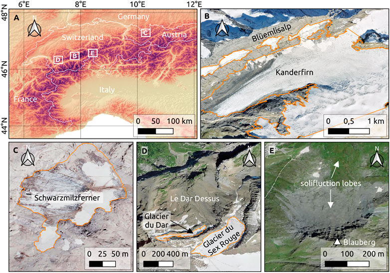
FIGURE 1. (A) Overview of the four study sites in the Alps where the UAV surveys were performed. (B) The Kanderfirn, a west-facing valley glacier in the Bernese Alps. The orange line indicates the glacier outline in 2018. (C) The Schwarzmilzferner, a southeast-facing avalanche-fed cirque glacier in the Allgäu Alps (glacier outline from 2020). (D) The north-facing cirque of Le Dar Dessus below the Glacier du Sex Rouge in the Vaud Alps (glacier outline from 2020). (E) The north-facing slope of the Blauberg, a mountain with active solifluction lobes at the northern margin of the Lepontine Alps. Data basis: void-filled SRTM elevation data (Reuter et al., 2007; Jarvis et al., 2008) (A); SWISSIMAGE from 2018 (B) and 2020 (D,E) provided by Swisstopo; Tiris orthophoto from 2020 provided by the Land Tirol (C).

2 Study Sites

2.1 Kanderfirn (Bernese Alps)

The Kanderfirn (46.477°N, 7.911°E) is a ca. 6 km long south-west-facing valley glacier located to the south of the Blüemlisalp Massif (3,661 m above sea level, a.s.l.) in the Bernese Alps (Figure 1). The glacier covers currently an elevation range from 2,300 to 3,200 m a.s.l. and an area of about 12 km². To monitor the long-term evolution of this glacier, multiple aerial surveys have been performed with a fixed-wing UAV each ablation season since 2017 (Groos et al., 2019). In addition to the geodetic surveys, ablation and surface lowering has been measured in-situ at twelve stakes along the central flow line since 2018. Snow accumulation was investigated for the first time in April 2021. A more detailed description of this study site is provided by Groos et al. (2019).

2.2 Schwarzmilzferner (Allgäu Alps)

The Schwarzmilzferner (47.297°N, 10.296°E) is a very small cirque glacier on the southeastern flank of the mountains Hochfrottspitze (2649 m a.s.l.) and Mädelegabel (2645 m a.s.l.) in the Allgäu Alps (Figure 1). Today, only a small ice patch is left. The elevation range is about 35 m (2410 m–2445 m) and the lateral extension reaches 260 m by 160 m, resulting in an area of about 30,000 m². The glacier was considerably larger in the recent past, reaching about 90,000 m² in 1985 (Schug and Kuhn, 1993). Despite its low elevation and a location exposed to sunshine during most of the day, very high precipitation rates (the annual mean is ca. 3,000 mm; the average snow accumulation in winter is ca. 2000 mm water equivalent) provide the basis for the existence of the glacier until today. Due to its unusual location, this very small glacier got into the focus of scientific interest. In the 1980s, first mass balance investigations were carried out, complemented by mapping its surface from aerial photogrammetry in 1971 and a terrestrial survey in 1985 (Mader, 1991). Since 1985, the glacier lost about two thirds of its area, while the surface elevation reduced by about 28 m.

2.3 Cirque of Le Dar Dessus (Vaud Alps)

The north-exposed and steep (mean slope ∼ 30°) cirque of Le Dar Dessus close to Les Diablerets (western Swiss Alps) has an area of about 1 km² and extends from ca. 2200–2700 m a.s.l. (Figure 1). About half of the cirque was glaciated at the end of the Little Ice Age (cf. Swiss Glacier Inventory SGI 1850, Maisch et al., 2000; Paul, 2004). Due to pronounced shrinkage, the glacier separated into two glaciers (Glacier du Dar and Glacier du Sex Rouge) around 1990 (cf. “journey through time”, Swisstopo). Only two small ice patches with a total area of about 30,000 m² in 2016 have remained in the upper part of the cirque (Linsbauer et al., 2021). Extensive sediment deposits of fine and coarser grain sizes as well as larger blocks of either glacial, gravitative or fluvially-reworked origin cover most of the area. Gravitational processes dominate in the upper part, both gravitative and fluvial processes in the middle part, and fluvial deposits in the lower part of the cirque. Several gullies point to the potential of fluvial erosion in the course of heavy precipitation events. In 2005, a debris flow of several 10⁴ m³ was released at ca. 2450 m a.s.l., which was the estimated lower limit of continuous permafrost at that time (Schoeneich and Consuegra, 2008). The disposition and probability of occurrence of proglacial and periglacial debris flows starting in the cirque of Le Dar Dessus are likely to increase in the future, due to both ongoing thawing of currently still frozen sediments and the assumed increase in the frequency and intensity of triggering precipitation events (Fischer and Keiler, 2019).

2.4 Blauberg Furkapass (Lepontine Alps)

The Blauberg (46.569° N, 8.418° E) is a 2768 m high mountain in the northernmost part of the Lepontine Alps south of the Furkapass, which connects the eastern and western Central Swiss Alps (Figure 1). The northern slope of the Blauberg covers an area of about 0.3 km² and extends from 2,300 m a.s.l. in the valley of the Furkareuss up to 2,760 m a.s.l. at the summit. From the valley up to an elevation of 2,430 m a.s.l., the ground is solely covered by alpine meadows. Above, the percentage of open scree increases steadily. Between 2,500 and 2,650 m a.s.l., open scree predominates. Rocks occur in small areas, but alpine meadows are absent here. The uppermost part of the site is dominated by bare rock. Seasonal ground frost prevailing up to 2,550 m a.s.l. and sporadic permafrost above characterise this periglacial landscape. The slope shape is overall conical and the overall longitudinal slope profile is concave with inclinations ranging from 15 to 53°. Within the area of loose debris, the slope is covered by solifluction lobes.

3 Data and Methods

3.1 UAV Surveys

Two different UAV models were deployed for the autonomous photogrammetric surveys (only the take-off and landing were performed manually) at the four study sites. We made use of a small and light-weight (730 g) commercial quadcopter (DJI Mavic Pro) equiped with a 12.35-megapixel camera to survey the Schwarzmilzferner and the steep cirque of Le Dar Dessus, where starting and landing of a fixed-wing UAV was difficult. The proprietary software Litchi (https://flylitchi.com/) served for mission planning and flight monitoring. For the larger UAV surveys on the Kanderfirn and on the northern slope of the Blauberg, we relied on a self-developed autonomous fixed-wing UAV, which was equipped with a 12-megapixel camera (GoPro Hero 5 Black). This fixed-wing UAV can survey an area of up to 1 km² per flight (for a detailed description of the aerial vehicle and system see Groos et al., 2019). The open-source software Paparazzi (Hattenberger et al., 2014) was used to programme and configure the autopilot of the fixed-wing UAV. Paparazzi also served for mission planning and flight monitoring. A detailed overview of all UAV surveys that were considered in this study for comparison with independent airborne and terrestrial datasets is provided in Table 1.

TABLE 1

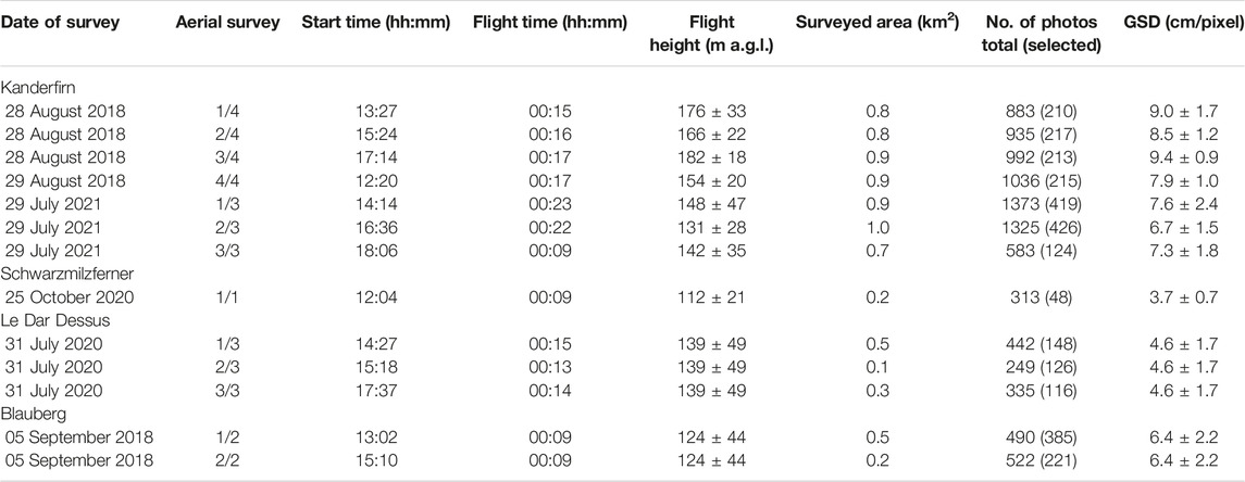
TABLE 1. Details of the conducted UAV surveys at each of the four study sites. The start of each survey is given in the local time (Central European Summer Time). GSD is the ground sampling distance.

3.2 GNSS Surveys

To accurately process and georeference the UAV images and to assess the quality of the produced orthophotos and DSMs (see Section 3.5), ground control points (GCPs) were surveyed at each study site. We generally placed red Teflon sheets (A2 paper size) on ice or snow and white Teflon sheets (same size) on bedrock, debris, and alpine meadows. The centre of each GCP was measured at each site (except Schwarzmilzferner) with a Trimble Geo 7X handheld dGNSS (Trimble, 2013). For the postprocessing of the dGNSS data, we relied on the Swiss Positioning Service (swipos) and the Automated GNSS Network for Switzerland (AGNES). The obtained mean horizontal accuracy was in the order of 10–20 cm and the mean vertical accuracy in the order of 20–30 cm. On 29 July 2021, a 620 m long cross-section profile running from northwest to southeast on the Kanderfirn was surveyed by dGNSS at an interval of about 30 m before the first UAV survey for comparison with the UAV DSM and the assessment of any large-scale distortions in the remote sensing product.

3.3 Geodetic Surveys at the Schwarzmilzferner

Surface area and surface elevation changes have been measured on a regular basis at the Schwarzmilzferner since 1999 at the end of each ablation season, usually in early October. During the first years, kinematic Global Positioning System (GPS) measurements provided information on profiles across the glacier and along its margin. These profiles were then interpolated to a glacier-wide grid using kriging as interpolation algorithm. Due to the high density of profiles and frequent crossing points, this method provided reliable elevation models of the ice surface. However, using only L1 GPS signals resulted in a vertical accuracy of about 0.5 m, despite including existing reference points outside of the glacier. Since 2011, a tachymeter is used to collect elevation information from about 500 locations across the surface by reflectorless laser measurements. The tachymeter is positioned on a reference point on nearby rock, which results in a measurement accuracy of less than 1 cm. Again, kriging is used for interpolation of the elevation model. The high number of measurements (1 measurement per 60 m²) guarantees a surface accuracy of a few centimetres. While the centre of the GCPs of the UAV surveys at the other study sites were measured with a handheld dGNSS, they were measured with the tachymeter on the Schwarzmilzferner. The interpolated tachymeter DSM from 25 October 2020 was used for comparison with the UAV DSM from the same day.

3.4 Airborne Orthophotos and Digital Surface Models

For the three study sites in the Swiss Alps (Kanderfirn, Le Dar Dessus, and Blauberg), high-resolution airborne orthophotos (SWISSIMAGE) and DSMs (swissALTI3D, swissSURFACE3D) from Swisstopo were used for comparison with the UAV data (see Table 2). The SWISSIMAGE (Level 3) is an orthomosaic available for the whole of Switzerland at a resolution of either 10 or 25 cm, depending on the region (Swiss Federal Office of Topography, 2020a). The orthomosaic is compiled of individual airborne photographs, has a positional accuracy of about 10 cm, and is updated every 3 years. Two different high-resolution elevation datasets exist for Switzerland: the swissALTI3D and the swissSURFACE3D. For areas above 2000 m, the swissALTI3D with a resolution of 50 cm is based on numerous airborne photographs that were processed using stereoscopic autocorrelation. The positional accuracy of the product is about ±1–3 m (Swiss Federal Office of Topography, 2021). From 2019 onward, the new swissSURFACE3D based on laser altimetry will successively replace the swissALTI3D. The swissSURFACE3D has a spatial resolution of 50 cm, a horizontal accuracy of ±20 cm, and vertical accuracy of ±10 cm (Swiss Federal Office of Topography, 2020b). We reprojected all photogrammetric products of Swisstopo from CH 1903 + LV95 (EPSG code: 2056) to WGS 84/UTM zone 32N (EPSG code: 32632). At the Schwarzmilzferner, we used the Tiris orthophoto of the Land Tirol with a resolution of 13 cm for comparison with the UAV orthophoto. The positional accuracy of the Tiris orthophoto is not specified.

TABLE 2

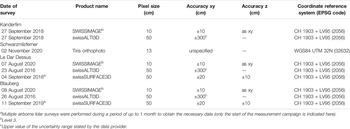
TABLE 2. Characteristics of the airborne orthophotos and DSMs used for comparison with the UAV data.

3.5 Generation of UAV Orthophotos and Digital Surface Models

We used the open-source photogrammetry software OpenDroneMap (www.opendronemap.org) in combination with the application programming interface WebODM (version 1.7) to process the aerial images from the different UAV surveys (for a detailed description of the entire workflow see Groos et al., 2019). OpenDronMap uses a structure-from-motion (SfM) and multi-view-stereo (MVS) approach to generate high-resolution orthophotos, DSMs, and 3D point clouds (Toffanin, 2019). We removed all non-nadir and low-altitude aerial photos and selected only every second or third photo from the original dataset (still guaranteeing a front image overlap of at least 70–80%) to reduce the computational cost of the photogrammetric processing. If multiple overlapping surveys were necessary to survey the entire study area, all selected aerial photos from the different flights were processed as one batch to obtain one consistent orthophoto and DSM per study site. For the accurate processing and georeferencing of the aerial photos, we created a GCP-file that lists the dGNSS position (X, Y, and Z coordinates) of each GCP measured in the field as well as the pixel coordinates of each associated aerial photo on which a GCP is visible (Toffanin, 2019). We used the default settings in WebODM apart from the following specifications to process the selected UAV photos: dsm = true (generates a DSM from the computed dense point cloud), dem-resolution = 20 (output resolution of the DSM set to 20 cm), orthophoto-resolution = 20 (output resolution of the orthophoto set to 20 cm), ignore-gsd = true (ignores the estimated ground sampling distance), optimize-disk-space = true (deletes heavy intermediate files to optimise disk space usage).

3.6 Accuracy Assessment

We used the position of the distributed red and white Teflon sheets that were measured with dGNSS in the field as a ground reference to assess the horizontal (XY) and vertical (Z) accuracy of each generated UAV orthophoto and DSM. In most cases, the red and white Teflon sheets can be identified as blurry or pixelated areas on the generated orthophotos. We measured the distance between the centre of each visible Teflon sheet and the actual position of the respective GCP manually in a geographic information system (GIS) to determine the offset at each GCP as well as the root-mean-square error of the entire orthophoto. This procedure is rather uncommon as the signalised points are in principle either used as GCPs or ground validation points (GVPs, i.e. reference points that were not used for the photogrammetric processing and georeferencing). However, as the number of Teflon sheets distributed in the field was relatively small, we did not split the population in GCPs and GVPs and therefore also did not consider any independent GVPs as in previous attempts (e.g. Rossini et al., 2018; Groos et al., 2019). Since these studies show that the mean offset calculated at GCPs and GVPs is usually similar, we can assume that the offset at the GCPs is more or less representative for the overall accuracy of the orthophoto. To determine the vertical accuracy, we compared the measured elevation at each GCP with the computed elevation in the associated pixel of the generated DSM. In addition, we analysed the elevation difference between dGNSS measurements on the Kanderfirn from 29 July 2021 and the DSM from the same date along a 620 m cross-section profile to verify how accurately the large-scale geometry of the terrain can be reproduced with the applied UAV-photogrammetry approach.

3.7 Data Comparison

To identify potential discrepancies between independently processed UAV data and airborne or terrestrial datasets, we compared the photogrammetric UAV products from the four study sites with high-resolution airborne orthophotos (see Table 2) as well as airborne and tachymeter DSMs. For the comparison of the UAV and airborne orthophotos and the assessment of the horizontal deviation, we identified up to 30 natural reference points at each study site such as boulders, cliffs, and crevasses that were clearly visible on both orthophotos. Analogous to the accuracy assessment using GCPs (see Section 3.6), we measured the relative offset between both orthophotos (UAV vs. airborne) at each reference point in a GIS. The calculated offset (i.e. root-mean square deviation) between multi-temporal products may be affected by surface displacements in the mountains, but we assume that this effect concerns solely the analysis at the Kanderfirn. For the three study sites in the Swiss Alps (Kanderfirn, Le Dar Dessus, and Blauberg), the UAV DSMs were compared with the airborne DSMs (i.e. swissALTI3D). At the Schwarzmilzferner, the tachymeter DSM from the same date as the UAV survey was used for comparison. For all study sites, we computed the DSM difference across the entire overlapping area of the compared DSMs (UAV DSM vs. swissALTI3D or tachymeter DSM). At the Kanderfirn, where a comparison across the glacier area is affected by surface lowering during the ablation season, we further distinguished between the elevation difference across the glacier area (“unstable” terrain) and off-glacier area (“stable” terrain). At the three other study sites (Le Dar Dessus, Schwarzmilzferner, and Blauberg), the elevation difference was computed separately for the area enclosing GCPs and the area without GCPs. As a reference, we also compared the swissALTI3D with the more accurate swissSURFACE3D (see Section 3.4) for the two study sites where lidar surveys have already been performed by Swisstopo (Le Dar Dessus and Blauberg).To check whether the deviation between the UAV and airborne products can be reduced using tie points over stable terrain, we reprocessed the UAV images of the Kanderfirn from 28/29 August 2018 with OpenDroneMap (see Section 3.5). In addition to the original 22 GCPs, we therefore also considered 10 boulders from the off-glacier area that were visible both on the SWISSIMAGE as well as on at least five individual UAV photos as tie points. Since these tie points were not measured by dGNSS in the field, we used the respective XY-coordinates from the SWISSIMAGE and the elevation from the swissALTI3D as a reference.

4 Results

4.1 Quality and Accuracy of the UAV Orthophotos and Digital Surface Models

In total, we performed 13 UAV surveys in complex (peri)glacial alpine terrain using fixed-wing and rotary-wing UAVs (Table 1). Based on the aerial images acquired during the UAV surveys, we could generate orthophotos and DSMs with a spatial resolution of 20 cm for all study areas using the open-source software OpenDroneMap. The SfM and MVS approach delivered consistent and gap-less orthophotos for various surface types present in the study areas, comprising exposed, snow-covered, and debris-covered glacier ice as well as bedrock, scree, and vegetation (Figure 2). The generated DSMs reproduce well the overall geometry of the investigated terrain and also capture characteristic geomorphological features such as medial moraines, supraglacial meltwater channels, and crevasses on the glacier (Figure 3B). However, other geomorphological features such as the solifluction lobes on the northern slope of the Blauberg that only rise by several decimetres above the surrounding surface are difficult to recognise in the UAV DSM (Figure 3E). Although the DSMs do not contain any real data gaps, artefacts (i.e. original voids that were not interpolated properly) have been detected in the DSMs of the Kanderfirn, Le Dar Dessus, and the Blauberg, but not in the DSM of the snow-covered Schwarzmilzferner. The smaller artefacts in the DSM of the Kanderfirn as well as the larger erroneous areas in the DSM of the Blauberg (see encircled areas in Figures 3B,E) originate most probably from insufficient lateral overlap (<50–70%) of the individual aerial photos.

FIGURE 2

FIGURE 2. High-resolution UAV orthophotos (pixel size = 20 cm) compiled from hundreds of individual UAV images (see Table 1) using OpenDroneMap. (A) Kanderfirn, 28/29 August 2018. Background image (outside the white perimeter): SWISSIMAGE Level 3 from 2018 (Swisstopo). (B) Kanderfirn, 29 July 2021. Background image: SWISSIMAGE Level 3 from 2018 (Swisstopo). (C) Schwarzmilzferner, 25 October 2020. Background image: Tiris orthophoto from 2020 (Land Tirol) (D) Le Dar Dessus, 31 July 2020. Background image: SWISSIMAGE Level 3 from 2020 (Swisstopo). (E) Blauberg, 5 September 2018. Background image: SWISSIMAGE Level 3 from 2020 (Swisstopo). The yellow-orange crosses indicate where the aerial images were acquired. GCPs = ground control points. RPs = reference points. At the ablation stakes, surface displacements and surface lowering has been measured repeatedly since 2018.

FIGURE 3

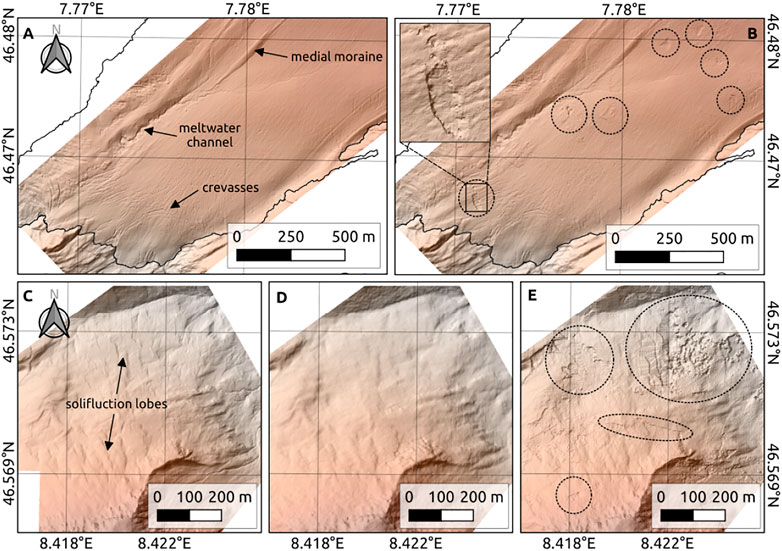
FIGURE 3. Compilation of hillshades created from different airborne and UAV DSMs. Reddish areas indicate higher elevations whereas greyish areas indicate lower elevations. (A) swissALTI3D of the Kanderfirn from 27 September 2018. (B) UAV DSM of the Kanderfirn from 28/29 August 2018. The dashed circles indicate deficiencies in the DSM that were not interpolated properly, most probably because of low image overlap or contrast. (C) swissSURFACE3D of the Blauberg from September 2019, (D) swissALTI3D of the Blauberg from 26 August 2016, and (E) UAV DSM of the Blauberg from 5 September 2018. The dashed circles indicate artefacts that probably originate from insufficient image overlap.

Using the GCPs distributed and measured with dGNSS in the field, we were able to assess the overall accuracy of the UAV orthophotos and DSMs. The absolute number of GCPs used for the processing and georeferencing of the aerial photos varied between 8 and 22 per site (translating into a density of 4–40 GCPs km⁻²), depending on the available time in the field and the accessibility of the terrain. The calculated horizontal and vertical root-mean-square error (RMSE) varies greatly between the four study sites (Table 3). At the two larger study sites (Kanderfirn and Blauberg), where the fixed-wing UAVs were deployed, the XY-RMSE ranges from 0.97 to 1.34 m and the Z-RMSE from 0.30 to 1.75 m. At the two smaller sites (Schwarzmilzferner and Le Dar Dessus), however, the horizontal and vertical RMSE is less than 0.30 m and, thus, in the order of the accuracy of the deployed dGNSS. The horizontal accuracy of the orthophotos is particularly dependent on the ground sampling distance (GSD) and therefore tends to decrease with increasing flight height (Figure 4).The cross-comparison between the UAV DSM and dGNSS measurements along a 620 m long cross-section profile on the Kanderfirn perpendicular to the flow-line reveals that the UAV DSM reflects well the overall geometry of the glacier (Figure 5A). Large-scale radial distortion towards the edges of the UAV DSM (often referred to as “warping”, “doming” or “fishbowling”) was not detected. However, the accuracy of the UAV DSM tends to slightly decrease towards the orographically left glacier margin (Figure 5B). The root-mean-square deviation of the UAV DSM elevations from the measured dGNSS elevations is 0.5 ± 0.5 m. At about 40% of the compared points along the cross-section profile, the deviation is less than the general dGNSS accuracy.

TABLE 3

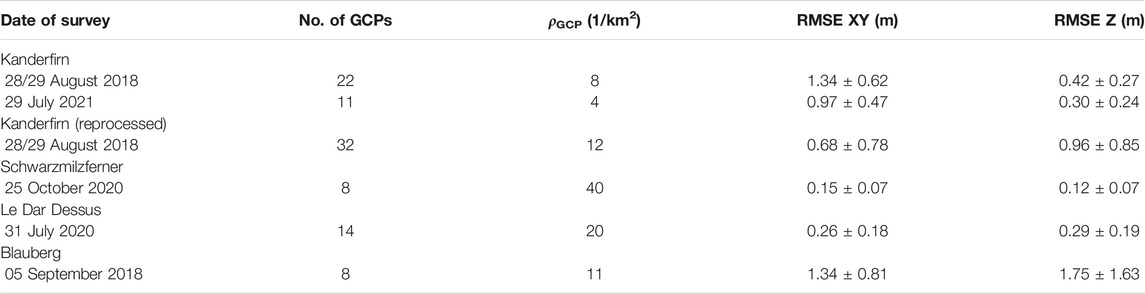
TABLE 3. Number of GCPs used for the processing of UAV images from each survey and for the validation of the individual UAV orthophotos and DSMs generated with WebODM. ρ_GCP is the density of GCPs per km² of surveyed area (the concept is described in more detail by Gindraux et al., 2017). The root-mean-square error (RMSE) (± standard deviation) indicates the lateral (XY) and vertical (Z) accuracy of the photogrammetric products as inferred from the deviation between the GCPs’ position (see Figure 2) measured by dGNSS and the XYZ position of the red and whity Teflon sheets visible on the orthophotos. Only 12 (out of 22) and 8 (out of 11) GCPs were used for the validation of the XY offsets of the Kanderfirn orthophotos from 28/29 August 2018 and 29 July 2021, respectively, as not all GCPs were found on the generated orthophotos.

FIGURE 4

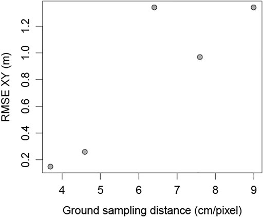
FIGURE 4. Relationship between ground sampling distance (GSD), which increases with flight height, and the root-mean-square error (RMSE) measured at the GCPs (see Tables 1, 2). The RMSE serves as measure for the overall orthophoto accuracy. Note that not only the GSD (i.e. flight height) affect orthophoto and DSM accuracy, but also other parameters such as GCP density.

FIGURE 5

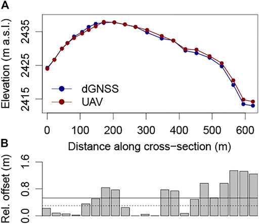
FIGURE 5. Surface elevation profile across the tongue of the Kanderfirn, perpendicular to the flow line, as inferred from dGNSS measurements and UAV photogrammetric surveys on 29 July 2021. (A) Comparison of the dGNSS and UAV-based surface elevation cross-section profiles. (B) Deviation between the 22 dGNSS measurements and the surface elevation at the same points extracted from the generated UAV DSM. The solid line represents the mean deviation and the dashed line the upper limit of the vertical accuracy of the dGNSS measurements (0.30 m). Note that the vertical deviation is largest near the orographically left glacier margin. In steeper areas, small horizontal offsets in the order of a few decimetres may result in relatively large vertical errors ($>$1 m).

4.2 Similarities and Discrepancies Between the Compared Datasets

The horizontal offset (Table 4) at selected reference points (see Figure 2) between the UAV and airborne orthophotos is larger than the positional accuracy (Table 3) of the UAV products themselves, thus indicating that the offset cannot be explained by the limited accuracy of the UAV products alone. The largest root-mean-square deviation (RMSD) of a UAV orthophoto from an airborne orthophoto was observed at the Kanderfirn (Table 4). Across the glacier area, the XY-RMSD is 3.33 ± 1.06 m. However, part of the deviation can be explained by the ice flow during the 1-month period between the acquisition date of the UAV orthophoto and the SWISSIMAGE Level 3 orthophoto (Table 1, 2). The mean surface displacement of the lower ablation zone of the Kanderfirn as measured with dGNSS at six ablation stakes (see Figure 2) in the period from end of August until end of September 2018 was 0.9 ± 0.5 m per month. Consequently, the XY-RMSD of 1.4 ± 0.8 m measured at three points in the stable terrain outside the glacier area seems a more realistic measure for the actual deviation. At the Schwarzmilzferner, for which the most accurate UAV orthophoto was obtained (XY-RMSE = 0.15 ± 0.07 m), the XY-RMSD relative to the Tiris orthophoto was 1.89 ± 0.81 m. Since most reference points were located across the off-glacier area (suitable reference objects on the ice were covered by snow), the XY-RMSD across the glacier area with GCPs might be smaller, but the general deviation may indicate a shift or distortion in the Tiris orthophoto.

TABLE 4

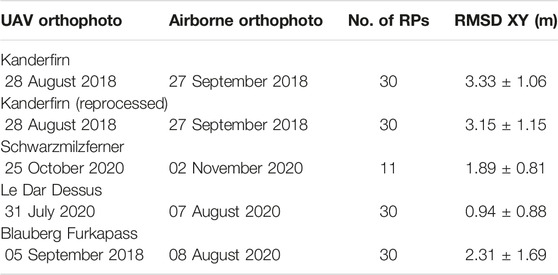
TABLE 4. Lateral offset (XY) between the UAV and airborne orthophotos at selected reference points (RPs) (see Figure 2). Natural objects such as boulders, cliffs, and crevasses that were visible on both orthophotos served as RPs and were used for determining the lateral root-mean-sqaure deviation (RMSD) between both products.

In the course of the analysis, we also detected a considerable distortion in the SWISSIMAGE (Level 3) from the Kanderfirn. The horizontal displacement was much larger than the general XY-accuracy of ±10 cm given by Swisstopo (Swiss Federal Office of Topography, 2020a). Compared to the UAV orthophotos, the swissALTI3D, and the SWISSIMAGE (Level 3) orthophoto from 2014 (not shown), the SWISSIMAGE (Level 3) orthophoto from 2018 is shifted by about 10 m to the north in the area close to the terminus (Figure 6). It is evident that the area of distortion is located at the margin of two different tiles (no. 2625_1145 and 2625_1146) of the swissALTI3D (Figure 6D) that was used for the orthorectification of the aerial photos (Swiss Federal Office of Topography, 2020a). The lower level of detail and poor interpolation of the swissALTI3D-tiles south of 46.4650°N may have caused larger uncertainties in the proglacial area of the Kanderfirn. However, it is not obvious why the SWISSIMAGE (Level 3) is distorted whereas the underlying swissALTI3D is not. This discrepancy reveals that also airborne orthophotos with the highest spatial resolution and accuracy that are currently available for alpine areas require an independent validation and quality check in mountainous terrain before comparison with other datasets.

FIGURE 6

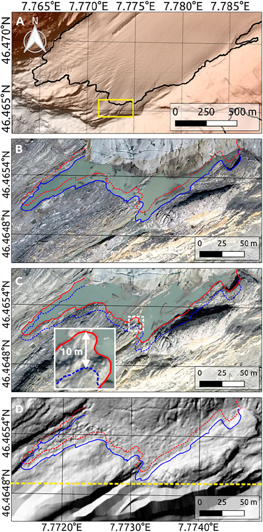
FIGURE 6. Horizontal displacement error in the SWISSIMAGE (Level 3) from 27 September 2018 at the terminus of the Kanderfirn. (A) Hillshade created from the swissALTI3D (27 September 2018). The yellow rectangle indicates the perimeter of the maps below (B–D). (B) UAV orthophoto from 28/29 August 2018. (C) SWISSIMAGE (Level 3) from 27 September 2018. (D) Hillshade created from the swissALTI3D. The dashed yellow line indicates the boundary between the high-resolution tile to the north (no. 2625_1145) and the poorly interpolated tile to the south (no. 2625_1146). The red line indicates the outline of the proglacial lake as seen on the SWISSIMAGE (Level 3) from 2018 and the blue line indicates the lake outline as seen on the UAV orthophoto, the swissALTI3D, and the SWISSIMAGE (Level 3) from 2014 (not shown).

Although both the UAV DSMs and the airborne and terrestrial DSMs reflect well the overall geometry of the four alpine study sites, there are discrepancies between the compared DSMs and inconsistencies within the individual DSMs. While the swissALTI3D does not contain any obvious artefacts (Figures 3A,D), the accuracy and level of detail may be decreased in areas where high-resolution aerial photos are not available in sufficient quantity (Figure 6D). Compared to the swissALTI3D, the sharpness and level of detail is further improved in the successor elevation product swissSURFACE3D, which is based on laser altimetry (cf. Figures 3C,D). The UAV DSMs have a similar level of detail as the swissALTI3D and capture characteristic geomorphological features (cf. Figures 3A,B), but they may contain artefacts in areas where the overlap or contrast of the acquired aerial photos is not sufficient (Figures 3B,E). The tachymeter DSM is very accurate in the centre of the study site (Section 3.3), but as it is based on the interpolation of individual point measurements, it has a lower level of detail than the UAV and airborne DSMs and becomes less accurate towards the edges of the dataset.

The aforementioned distortions and artefacts in the individual DSMs are one major reason for the discrepancies between the compared datasets from the same sites (Figure 7). Another reason is the missing co-registration of the DSMs. A small horizontal shift between the compared DSMs from the same site may cause a large vertical error (i.e. elevation difference) especially in steep terrain (larger dashed circle in Figure 7D). The smallest deviation in surface elevation was therefore observed at the Schwarzmilzferner where individual laser measurements served both for the generation of the tachymeter DSM and the georeferencing of the UAV DSM (Figures 7C, 8C). Despite the general discrepancies and artefacts, spatio-temporal surface elevation changes associated with the melting of glacier ice (Figures 7A,B and Figures 8A,B) or the accumulation of snow and avalanche deposits (black ovals in Figures 7B,D) can be mapped using multi-temporal DSMs. The mean surface elevation change across the tongue of the Kanderfirn derived from DSM differencing for the period from 28/29 August to 27 September 2018 (−1.4 ± 0.8 m) is similar to the ice-flow-corrected elevation change for the same period (−1.1 ± 0.1 m) measured by dGNSS at four ablation stakes (Figure 2). The same holds true for the mean glacier surface elevation change between 28/29 August 2018 and 29 July 2021 (Figures 7B, 8B) measured by DSM differencing (−7.5 ± 2.2 m) and dGNSS (−7.3 ± 1.9 m; n = 4). However, the dataset comparison shows that considerable uncertainties remain in the UAV DSMs in areas without GCPs (e.g., Figures 7B, 8B), in areas with few or unevenly distributed GCPs (e.g., Figures 7D, 8D), and in areas with low image contrast and low lateral image overlap ($<$50–70%) (e.g., Figures 7E, 8E).

FIGURE 7

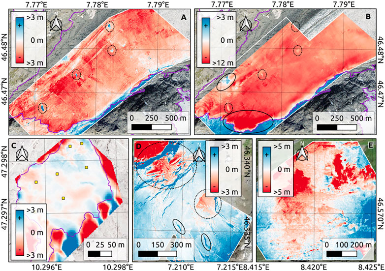
FIGURE 7. Surface elevation difference between the UAV DSMs and airborne or terrestrial DSMs. The purple lines indicate glacier boundaries (A–C). (A) Kanderfirn: swissALTI3D 2018-09-27 minus UAV DSM 2018-08-28/29. The dashed circles indicate the most prominent artefacts in the UAV DSM. Note that the predominantly negative elevation change (i.e. surface lowering) is the result of melting from end of August until end of September 2018. (B) Kanderfirn: UAV DSM 2021-07-29 minus UAV DSM 2018-08-28/29. The black ovals indicate areas of pronounced surface elevation change. The positive elevation changes (encircled blue area) originate from increased avalanche activity during winter 2020/2021, whereas the surface lowering (encircled red area) at the tongue is the result of itense melting between 2018 and 2021. (C). Schwarzmilzferner: UAV DSM 2020-10-25 minus Tachymeter DSM 2020-10-25. Note that the difference between both DSMs is relatively small on the glacier where GCPs (yellow squares) were distributed. However, the elevation difference increases rapidly outside the glacier area, which was not surveyed with the tachymeter. (D) Le Dar Dessus: UAV DSM 2020-07-31 minus swissALTI3D 2016-08-23. The dashed circles indicate very steep areas (i.e. cliffs with a slope of 30-90°) where small horizontal offsets between the DSMs result in large elevation differences ($>$1 m). The black ovals indicate gullies that were filled by snow in 2020, but not in 2016. (E) Blauberg: UAV DSM 2018-09-05 minus swissALTI3D 2016-08-26. The large elevation differences, especially in the lower (i.e. northern) part of the slope, originate from inaccuracies in the UAV DSM.

FIGURE 8

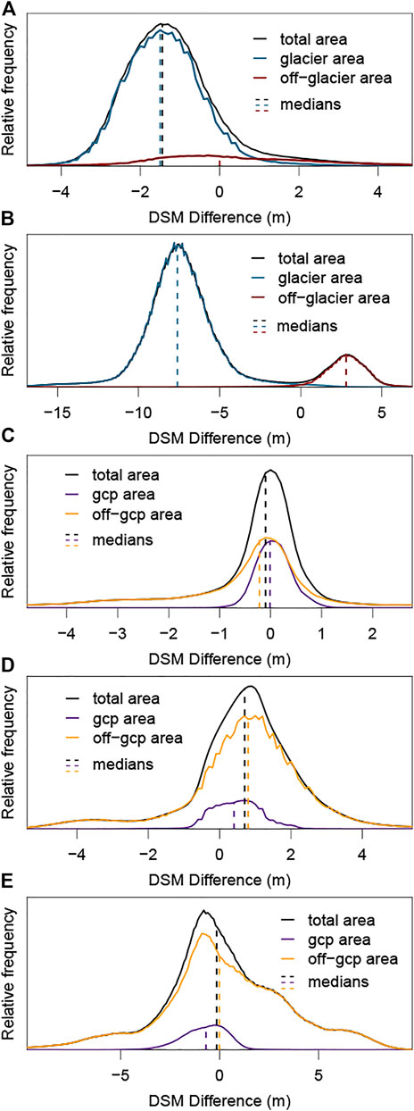
FIGURE 8. Frequency distribution of the pixel-based elevation difference between the UAV DSMs and airborne or terrestrial DSMs. (A) Kanderfirn: swissALTI3D 2018-09-27 minus UAV DSM 2018-08-28/29. (B) Kanderfirn: UAV DSM 2021-07-21 minus UAV DSM 2018-08-28/29. Note that the curve and median of the total area and glacier area overlap. (C). Schwarzmilzferner: UAV DSM 2020-10-25 minus Tachymeter DSM 2020-10-25. (D) Le Dar Dessus: UAV DSM 2020-07-31 minus swissALTI3D 2016-08-23. (E) Blauberg: UAV DSM 2018-09-05 minus swissALTI3D 2016-08-26. For subfigures (A) and (B), the elevation difference distribution was computed separately for the glacier area and off-glacier area. For subfigures (C–E), the elevation difference distribution was computed separately for the area enclosing GCPs (see Figure 2) and the area without GCPs.

As the test at the Kanderfirn shows, considering additional tie points in stable terrain can help reduce the deviation between multiple DSMs from the same site. Reprocessing the UAV images from 28/29 August 2018 with additional tie points from outside the glacier area improved the horizontal (XY) accuracy of the UAV DSM (Table 3) and minimally decreased the elevation difference to the swissALTI3D in the proglacial area (cf. Figures 9A,B). However, the drawback of using additional tie points from the off-glacier area for the generation of a DSM is the potential feedback on the reconstructed glacier geometry. In our example, the exclusive use of additional tie points along the orographically left glacier margin due to the lack of aerial photos of stable terrain along the orographically right glacier margin led to a slight tilting of the UAV DSM. In direct comparison with the swissALTI3D, the tilting caused an amplified surface lowering along the right glacier margin and an unrealistic uplift along the orographically left glacier margin (Figure 9B).

FIGURE 9

FIGURE 9. Surface elevation difference at the Kanderfirn between 28/29 August and 27 September 2018. (A) swissALTI3D minus UAV DSM (as in Figure 7A). (B) swissALTI3D minus reprocessed UAV DSM using additional tie points along the orographically left glacier margin and in the proglacial area.

5 Discussion

The accuracy assessment of the generated UAV orthophotos and DSMs shows that UAV photogrammetry is generally well suited for characterising and analysing surface processes and changes in (peri)glacial alpine terrain. However, some of the discrepancies observed between the compared UAV, airborne, and terrestrial data originate from inaccuracies and artefacts in the UAV products and emphasise the need to further improve the methodology, from data collection to data processing. While some of the typical error sources in UAV photogrammetry such as insufficient image overlap are independent of the study area, other possible error sources such as low image contrast (e.g., in snow-covered areas) or small number of GCPs (e.g., in rugged terrain) are generic for aerial surveys in the mountains. Another challenge related to UAV and terrestrial photogrammetry and lidar in the mountains is the often limited area of stable terrain that is required for the co-registration of multi-temporal datasets (e.g., Immerzeel et al., 2014; Fischer et al., 2016; Piermattei et al., 2016). The aim of the following discussion is to identify typical error sources and pitfalls in UAV photogrammetry in alpine terrain, outline how they can be avoided, and elaborate best practices for the fusion of spatial data from different dates and platforms based on the findings from the multi-dataset comparison.

One main factor controlling the accuracy of UAV products in mountain environments is the GCP density. At our four study sites, the GCP density ranged from 8 to 40 GCPs km⁻². According to Gindraux et al. (2017), a density of more than 10 GCP km⁻² should be sufficient to generate orthophotos and DSMs with a decimetre accuracy. The accuracies (RMSEs) we obtained for the four alpine study sites vary between less than 15 cm and more than 100 cm (Table 3). In other studies, accuracies of 10–15 cm have been reported (e.g., Rossini et al., 2018), but in this case the surveyed area was relatively small ($<$0.7 km²) and the GCP density very high ($>$120 GCPs km⁻²). Besides GCP density, also the GCP distribution affects the orthophoto and DSM accuracy. While an even distribution would be ideal, this is often not feasible in alpine terrain as certain areas are inaccessible or too dangerous to distribute GCPs (e.g., Van Tricht et al., 2021). Inaccessibility of the terrain was also the reason for the uneven distribution of GCPs in the north-facing cirque of Le Dar Dessus below the Glacier du Sex Rouge (Figure 2D). Another reason for the insufficient number or distribution of GCPs may be limited time during field work.

Other important factors regarding the accuracy of UAV photogrammetric products are image resolution (i.e. GSD), image coverage, and image overlap, all related to flight height, as well as image contrast. The image matching during the photogrammetric processing is usually hampered in those areas in the mountains which are covered by fresh snow (e.g., Gindraux et al., 2017; Van Tricht et al., 2021). The low contrast leads to a reduced number of matching keypoints and, thus, causes inaccuracies and artefacts in the UAV products. However, the accurate and consistent UAV orthophoto and DSM from the snow-covered Schwarzmilzferner (Figure 2C) show that snow after being exposed to sunlight or rain has enough texture to allow for image matching and alignment. This finding is also supported by other studies (e.g., Bühler et al., 2016; Gindraux et al., 2017). The reasons for insufficient image overlap or coverage can be manifold. In deeply incised valleys, surveying areas along steep rock faces (such as the Blüemlisalp to the north of the Kanderfirn; Figure 1B) may be infeasible because of strong slope winds and limited GNSS accuracy. Insufficient image overlap may originate from large distances between adjacent flight paths (see for example Figures 2E, 3E) or from infrastructure in the mountains that must be circumvented. This was the case in the area of Le Dar Dessus where a cable car between La Tête aux Chamois and Le Sex Rouge crosses the surveyed cirque (see increased space between flight paths in the middle of Figure 2D). As the accuracy of UAV products is essential for quantitative analysis and comparison with other datasets, improving the methodology is necessary.

While some of the aforementioned challenges are inherent to UAV photogrammetry in the mountains, other limitations can be overcome. Careful flight-planning provides the basis for the acquisition of aerial photos with sufficient lateral overlap ($>$70–80%) and is essential to find an adequate compromise between a high image resolution (i.e. small GSD), a complete coverage of the area of interest, and a reasonable flight time. To be able to perform an accuracy assessment and co-register multi-temporal UAV orthophotos and DSMs, it is highly recommended to survey also stable terrain outside the (peri)glacial areas when studying surface processes and changes in the mountains (e.g., Immerzeel et al., 2014; Rossini et al., 2018; Groos et al., 2019; Van Tricht et al., 2021). A solution to increase the accuracy in areas covered by fresh snow is the enhancement of the image contrast through the use of multi-spectral cameras with a near infrared band (Bühler et al., 2017). The even distribution of sufficient GCPs both in the dynamic area and surrounding stable terrain is a prerequisite to obtain accurate UAV orthophotos and DMSs (Gindraux et al., 2017). Distinct natural features (serving as GCPs) in stable, but inaccessible, terrain might be measured with a tachymeter or similar device from reachable spots. An alternative to the distribution of GCPs in rugged terrain is the use of UAVs with a high-precision differential GNSS onboard (e.g., Chudley et al., 2019; Zhang et al., 2019; Stott et al., 2020; Van Tricht et al., 2021).

Besides the potential improvements in UAV photogrammetry discussed before, the evaluation and co-registration of multi-temporal orthophotos and DSMs (from different platforms) is key for the accurate analysis of surface displacements and surface elevation changes in alpine terrain. The displacement error discovered by chance in the SWISSIMAGE (Level 3) of the Kanderfirn (Figure 6) underlines the need for a careful quality check of external datasets used for comparison with UAV data. In steep terrain, small horizontal shifts between datasets may result in large vertical elevation change errors as the DSM difference map of Le Dar Dessus illustrates (Figure 7D). The processing steps for the co-registration of spatial data from different dates and platforms vary depending on the type of data that are available (Figure 10). In the optimal case, the raw data (i.e. aerial photos) of consecutive UAV or airborne surveys are processed along with GCPs or high-precision GNSS data to generate accurate orthophotos and DSMs (Figure 10). Common GCPs (i.e. tie points) in stable terrain may serve for the accurate co-registration of multi-temporal datasets (e.g., Immerzeel et al., 2014; Kraaijenbrink et al., 2018). If no GCPs or high-precission GNSS data are available, the original aerial photos can only be processed and co-registered using tie points in stable terrain (e.g., Benoit et al., 2019; Fu et al., 2021).

FIGURE 10

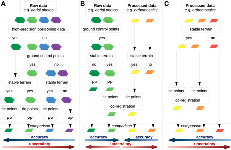
FIGURE 10. Overview of potential processing steps required for the analysis and comparison of multi-temporal UAV, airborne, satellite, or terrestrial data from the same location in (peri)glacial alpine terrain. The data processing differs depending on whether only the processed data (i.e. orthomosaics or DSMs) or also the raw data (i.e. individual aerial photos) are available. Green to violet rectangles indicate raw data whereas yellow to red rectangles indicate processed data. (A) Comparison of raw data from one or multiple platforms. If the original aerial photos from UAV or airborne surveys are available, GCPs and tie points in stable terrain can be directly used during the photogrammetric processing (PP) to align orthophotos or DSMs from differents dates. (B) Comparison of raw and processed data from different sources (e.g. UAV vs. airborne or satellite data). Tie points in stable terrain may serve for the co-registration of multi-temporal orthophotos or DSMs. (C) Comparison of processed data. Tie points in stable terrain may serve for the co-registration of multi-temporal orthophotos or DSMs. Without high-precision positioning data, GCPs, or tie points, the comparison of data from different dates or platforms is fraught with great uncertainties.

Instead of processing aerial photos from different dates independently, latest studies promote the photogrammetric processing of multi-temporal images in a single block to further increase the accuracy (Feurer and Vinatier, 2018; Cook and Dietze, 2019; Zhang et al., 2020). The new method makes use of keypoint detection algorithms such as the scale invariant feature transform (SIFT) and assumes that a certain number of matching keypoints in the photos (restricted to stable terrain) is invariant in space and time. This means that keypoints automatically detected in the photos from different dates are used to align the multi-temporal point clouds across stable terrain before 3D changes (in dynamic areas) are quantified through DSM differencing (Feurer and Vinatier, 2018). However, if only processed datasets such as airborne orthophotos and DSMs are available for a multi-temporal comparison, established co-registration tools can be used to match the multi-temporal datasets (Scheffler et al., 2017). As aerial photos of the stable terrain are generally a prerequisite for accurate co-registration of multi-temporal datasets (Figure 10), extending the UAV surveys beyond the primary area of interest is of utmost importance in dynamic mountain environments despite the associated challenges. In addition, UAVs equipped with a multi-spectral camera and a high-precision dGNSS are recommended to obtain the data accuracy needed for studying surface processes and 3D changes in alpine terrain.

6 Conclusion

In our study, we assessed the accuracy of UAV photogrammetry in (peri)glacial alpine terrain by comparing high-resolution UAV orthophotos and DSMs with airborne and terrestrial datasets at four alpine study sites with different topographic settings. The generated UAV products reflect the overall geometry of the investigated sites and also depict characteristic geomorphological features. However, the observed accuracy varies considerably between the study sites as the comparison with in-situ dGNSS measurement shows. The most accurate UAV products (RMSD $<$15 cm) were obtained at the smallest study site (0.2 km²) with a high GCP density (40 GCPs km⁻²) and sufficient image overlap and contrast, whereas lower accuracies (RMSD $>$100 cm) and artefacts associated with a low GCP density ($<$15 GCPs km⁻²) and insufficient lateral image overlap ($<$50–70%) were observed when more extensive areas were surveyed ($>$2.5 km²). As the low image contrast (e.g. in snow-covered areas) and the uneven distribution of GCPs (e.g. in rugged terrain) are inherent to UAV photogrammetry in the mountains, the use of UAVs equipped with multispectral cameras and high-precission dGNSS is recommended to improve the mapping accuracy. The comparison of multi-temporal UAV, airborne, and terrestrial datasets enabled the investigation of surface elevation changes, but the analysis also revealed considerable discrepancies in the datasets. The discrepancies originate both from distortions and artefacts in the UAV orthophotos and DSMs and from deficiencies in the external airborne datasets. Small horizontal shifts can result in large vertical surface elevation change errors in steep terrain. An accurate co-registration of multi-temporal UAV, airborne, and terrestrial data using tie points in stable terrain is therefore of utmost importance when it comes to the investigation of surface displacements and surface elevation changes in the high mountains.

Data Availability Statement

The raw data supporting the conclusion of this article will be made available by the authors, without undue reservation.

Author Contributions

AG designed the study. AG, MF, CM, and AS-R coordinated the fieldwork at the different study sites. AG performed the aerial surveys with the support of all authors. CM conducted the terrestrial geodetic survey. AG, RA, NK, and CM analysed the data and generated the orthophotos and digital surface models. AG created the figures and drafted the manuscript with contributions from MF, CM, and AS-R. All authors contributed to the final version of the manuscript.

Funding

The expenses for the fieldwork on the Kanderfirn, in the cirque of Le Dar Dessus, and on the Blauberg in the Swiss Alps were covered by the Institute of Geography of the University of Bern. The fieldwork on the Schwarzmilzferner in the Allgäu Alps was financed by the Geodesy and Glaciology group of the Bavarian Academy of Sciences and Humanities. Open access funding was provided by the University Of Bern.

Conflict of Interest

The authors declare that the research was conducted in the absence of any commercial or financial relationships that could be construed as a potential conflict of interest.

Publisher’s Note

All claims expressed in this article are solely those of the authors and do not necessarily represent those of their affiliated organizations, or those of the publisher, the editors and the reviewers. Any product that may be evaluated in this article, or claim that may be made by its manufacturer, is not guaranteed or endorsed by the publisher.

Acknowledgments

We would like to thank Thalia Bertschinger, Nicolas Brand, Sabrina Erlwein, Nicole Fahrni, Lars Imbach, Ann Christin Kogel, Astrid Lambrecht, Simon Mägli, Carla Padovan, Alexis Rüeger, and Lorenz Zeller for support during the fieldwork at the different study sites. We are also grateful to Saliba Saliba and Manuel Bart for their technical support with WebODM. Special thanks go to Sinh Marc Ly and Mira Barben for their assistance in analysing the data.

References

Avian, M., Bauer, C., Schlögl, M., Widhalm, B., Gutjahr, K.-H., Paster, M., et al. (2020). The Status of Earth Observation Techniques in Monitoring High Mountain Environments at the Example of Pasterze Glacier, Austria: Data, Methods, Accuracies, Processes, and Scales. Remote Sens. 12, 1251. doi:10.3390/rs12081251

CrossRef Full Text | Google Scholar

Benoit, L., Gourdon, A., Vallat, R., Irarrazaval, I., Gravey, M., Lehmann, B., et al. (2019). A High-Resolution Image Time Series of the Gorner Glacier - Swiss Alps - Derived from Repeated Unmanned Aerial Vehicle Surveys. Earth Syst. Sci. Data 11, 579–588. doi:10.5194/essd-11-579-2019

CrossRef Full Text | Google Scholar

Bhardwaj, A., Sam, L., AkankshaMartín-Torres, F. J., Martín-Torres, F. J., and Kumar, R. (2016). UAVs as Remote Sensing Platform in Glaciology: Present Applications and Future Prospects. Remote Sens. Environ. 175, 196–204. doi:10.1016/j.rse.2015.12.029

CrossRef Full Text | Google Scholar

Bühler, Y., Adams, M. S., Bösch, R., and Stoffel, A. (2016). Mapping Snow Depth in Alpine Terrain with Unmanned Aerial Systems (UASs): Potential and Limitations. Cryosphere 10, 1075–1088. doi:10.5194/tc-10-1075-2016

CrossRef Full Text | Google Scholar

Bühler, Y., Adams, M. S., Stoffel, A., and Boesch, R. (2017). Photogrammetric Reconstruction of Homogenous Snow Surfaces in Alpine Terrain Applying Near-Infrared UAS Imagery. Int. J. Remote Sens. 38, 3135–3158. doi:10.1080/01431161.2016.1275060

CrossRef Full Text | Google Scholar

Chudley, T. R., Christoffersen, P., Doyle, S. H., Abellan, A., and Snooke, N. (2019). High-accuracy UAV Photogrammetry of Ice Sheet Dynamics with No Ground Control. Cryosphere 13, 955–968. doi:10.5194/tc-13-955-2019

CrossRef Full Text | Google Scholar

Cook, K. L., and Dietze, M. (2019). Short Communication: A Simple Workflow for Robust Low-Cost UAV-Derived Change Detection without Ground Control Points. Earth Surf. Dynam. 7, 1009–1017. doi:10.5194/esurf-7-1009-2019

CrossRef Full Text | Google Scholar

Dąbski, M., Zmarz, A., Pabjanek, P., Korczak-Abshire, M., Karsznia, I., and Chwedorzewska, K. J. (2017). UAV-based Detection and Spatial Analyses of Periglacial Landforms on Demay Point (King George Island, South Shetland Islands, Antarctica). Geomorphology 290, 29–38. doi:10.1016/j.geomorph.2017.03.033

CrossRef Full Text | Google Scholar

Feurer, D., and Vinatier, F. (2018). Joining Multi-Epoch Archival Aerial Images in a Single SfM Block Allows 3-D Change Detection with Almost Exclusively Image Information. ISPRS J. Photogrammetry Remote Sens. 146, 495–506. doi:10.1016/j.isprsjprs.201810.1016/j.isprsjprs.2018.10.016

CrossRef Full Text | Google Scholar

Fischer, M., Huss, M., Kummert, M., and Hoelzle, M. (2016). Application and Validation of Long-Range Terrestrial Laser Scanning to Monitor the Mass Balance of Very Small Glaciers in the Swiss Alps. Cryosphere 10, 1279–1295. doi:10.5194/tc-10-1279-2016

CrossRef Full Text | Google Scholar

Fischer, M., and Keiler, M. (2019). “Implications of the rapid disappearance of glacier du sex rouge (western swiss alps) for local multi-hazard and risk assessment at les diablerets,” in Geophysical Research Abstracts, 21.

Google Scholar

Fu, Y., Liu, Q., Liu, G., Zhang, B., Zhang, R., Cai, J., et al. (2021). Seasonal Ice Dynamics in the Lower Ablation Zone of Dagongba Glacier, Southeastern Tibetan Plateau, from Multitemporal UAV Images. J. Glaciol. 1–15. doi:10.1017/jog.2021.123

CrossRef Full Text | Google Scholar

Fugazza, D., Scaioni, M., Corti, M., D'Agata, C., Azzoni, R. S., Cernuschi, M., et al. (2018). Combination of UAV and Terrestrial Photogrammetry to Assess Rapid Glacier Evolution and Map Glacier Hazards. Nat. Hazards Earth Syst. Sci. 18, 1055–1071. doi:10.5194/nhess-18-1055-2018

CrossRef Full Text | Google Scholar

Gaffey, C., and Bhardwaj, A. (2020). Applications of Unmanned Aerial Vehicles in Cryosphere: Latest Advances and Prospects. Remote Sens. 12, 948. doi:10.3390/rs12060948

CrossRef Full Text | Google Scholar

Gindraux, S., Boesch, R., and Farinotti, D. (2017). Accuracy Assessment of Digital Surface Models from Unmanned Aerial Vehicles' Imagery on Glaciers. Remote Sens. 9, 186. doi:10.3390/rs9020186

CrossRef Full Text | Google Scholar

Glasser, N. F., Roman, M., Holt, T. O., Žebre, M., Patton, H., and Hubbard, A. L. (2020). Modification of Bedrock Surfaces by Glacial Abrasion and Quarrying: Evidence from North Wales. Geomorphology 365, 107283. doi:10.1016/j.geomorph.2020.107283

CrossRef Full Text | Google Scholar

Groos, A. R., Bertschinger, T. J., Kummer, C. M., Erlwein, S., Munz, L., and Philipp, A. (2019). The Potential of Low-Cost UAVs and Open-Source Photogrammetry Software for High-Resolution Monitoring of Alpine Glaciers: A Case Study from the Kanderfirn (Swiss Alps). Geosciences 9, 356. doi:10.3390/geosciences9080356

CrossRef Full Text | Google Scholar

Hattenberger, G., Bronz, M., and Gorraz, M. (2014). “Using the Paparazzi UAV System for Scientific Research,” in IMAV 2014, International Micro Air Vehicle Conference and Competition (Delft, Netherlands: Delft University of Technology), 247–252. doi:10.4233/UUID%3AB38FBDB7-E6BD-440D-93BE-F7DD1457BE60

CrossRef Full Text | Google Scholar

Immerzeel, W. W., Kraaijenbrink, P. D. A., Shea, J. M., Shrestha, A. B., Pellicciotti, F., Bierkens, M. F. P., et al. (2014). High-resolution Monitoring of Himalayan Glacier Dynamics Using Unmanned Aerial Vehicles. Remote Sens. Environ. 150, 93–103. doi:10.1016/j.rse.2014.04.025

CrossRef Full Text | Google Scholar

James, M. R., and Robson, S. (2014). Mitigating Systematic Error in Topographic Models Derived from UAV and Ground-Based Image Networks. Earth Surf. Process. Landf. 39, 1413–1420. doi:10.1002/esp.3609

CrossRef Full Text | Google Scholar

Jarvis, A., Reuter, H. I., Nelson, A., and Guevara, E. (2008). Hole-filled SRTM for the Globe Version 4, Available from the CGIAR-CSI SRTM 90m Database. Available at: http://srtm.csi.cgiar.org (Accessed November 5, 2021)

Google Scholar

Jouvet, G., Weidmann, Y., Seguinot, J., Funk, M., Abe, T., Sakakibara, D., et al. (2017). Initiation of a Major Calving Event on the Bowdoin Glacier Captured by UAV Photogrammetry. Cryosphere 11, 911–921. doi:10.5194/tc-11-911-2017

CrossRef Full Text | Google Scholar

Kraaijenbrink, P. D. A., Shea, J. M., Litt, M., Steiner, J. F., Treichler, D., Koch, I., et al. (2018). Mapping Surface Temperatures on a Debris-Covered Glacier with an Unmanned Aerial Vehicle. Front. Earth Sci. 6, 1–19. doi:10.3389/feart.2018.00064

CrossRef Full Text | Google Scholar

Kraaijenbrink, P. D. A., Shea, J. M., Pellicciotti, F., Jong, S. M. d., and Immerzeel, W. W. (2016). Object-based Analysis of Unmanned Aerial Vehicle Imagery to Map and Characterise Surface Features on a Debris-Covered Glacier. Remote Sens. Environ. 186, 581–595. doi:10.1016/j.rse.2016.09.013

CrossRef Full Text | Google Scholar

Linsbauer, A., Huss, M., Hodel, E., Bauder, A., Fischer, M., Weidmann, Y., et al. (2021). The New Swiss Glacier Inventory SGI2016: From a Topographical to a Glaciological Dataset. Front. Earth Sci. 9, 22. doi:10.3389/feart.2021.704189

CrossRef Full Text | Google Scholar

Mader, R. (1991). Der Schwarzmilzferner in Den Allgäuer Alpen. Z. für Gletscherkd. Glazialgeol. 27/28, 139–144.

Google Scholar

Maisch, M., Wipf, A., Denneler, B., Battaglia, J., and Benz, C. (2000). “Die Gletscher der Schweizer Alpen: Gletscherhochstand 1850, Aktuelle Vergletscherung, Gletscherschwund-Szenarien (Schlussbericht NFP 31). 2. Auflage,” in vdf Hochschulverlag an der ETH Zürich (Zürich, Switzerland: vdf Hochschulverlag an der ETH Zürich).

Google Scholar

Mather, A., Fyfe, R., Clason, C., Stokes, M., Mills, S., and Barrows, T. (2019). Automated Mapping of Relict Patterned Ground: An Approach to Evaluate Morphologically Subdued Landforms Using Unmanned-Aerial-Vehicle and Structure-From-Motion Technologies. Prog. Phys. Geogr. Earth Environ. 43, 174–192. doi:10.1177/0309133318788966

CrossRef Full Text | Google Scholar

Paul, F. (2004). The New Swiss Glacier Inventory 2000 – Application of Remote Sensing and GIS (Zürich, Switzerland: Department of Geography, University of Zurich), 52. PhD Thesis. Schriftenreihe Physische Geographie.

Piermattei, L., Carturan, L., de Blasi, F., Tarolli, P., Dalla Fontana, G., Vettore, A., et al. (2016). Suitability of Ground-Based SfM-MVS for Monitoring Glacial and Periglacial Processes. Earth Surf. Dynam. 4, 425–443. doi:10.5194/esurf-4-425-2016

CrossRef Full Text | Google Scholar

Piermattei, L., Carturan, L., and Guarnieri, A. (2015). Use of Terrestrial Photogrammetry Based on Structure-From-Motion for Mass Balance Estimation of a Small Glacier in the Italian Alps. Earth Surf. Process. Landf. 40, 1791–1802. doi:10.1002/esp.3756

CrossRef Full Text | Google Scholar

Reuter, H. I., Nelson, A., and Jarvis, A. (2007). An Evaluation of Void-filling Interpolation Methods for SRTM Data. Int. J. Geogr. Inf. Sci. 21, 983–1008. doi:10.1080/13658810601169899

CrossRef Full Text | Google Scholar

Rossini, M., Di Mauro, B., Garzonio, R., Baccolo, G., Cavallini, G., Mattavelli, M., et al. (2018). Rapid Melting Dynamics of an Alpine Glacier with Repeated UAV Photogrammetry. Geomorphology 304, 159–172. doi:10.1016/j.geomorph.2017.12.039

CrossRef Full Text | Google Scholar

Ryan, J. C., Hubbard, A., Box, J. E., Brough, S., Cameron, K., Cook, J. M., et al. (2017). Derivation of High Spatial Resolution Albedo from UAV Digital Imagery: Application over the Greenland Ice Sheet. Front. Earth Sci. 5, 1–13. doi:10.3389/feart.2017.00040

CrossRef Full Text | Google Scholar

Ryan, J. C., Hubbard, A. L., Box, J. E., Todd, J., Christoffersen, P., Carr, J. R., et al. (2015). UAV Photogrammetry and Structure from Motion to Assess Calving Dynamics at Store Glacier, a Large Outlet Draining the Greenland Ice Sheet. Cryosphere 9, 1–11. doi:10.5194/tc-9-1-2015

CrossRef Full Text | Google Scholar

Šašak, J., Gallay, M., Kaňuk, J., Hofierka, J., and Minár, J. (2019). Combined Use of Terrestrial Laser Scanning and UAV Photogrammetry in Mapping Alpine Terrain. Remote Sens. 11, 2154. doi:10.3390/rs11182154

CrossRef Full Text | Google Scholar

Scheffler, D., Hollstein, A., Diedrich, H., Segl, K., and Hostert, P. (2017). AROSICS: An Automated and Robust Open-Source Image Co-registration Software for Multi-Sensor Satellite Data. Remote Sens. 9, 676. doi:10.3390/rs9070676

CrossRef Full Text | Google Scholar

Schoeneich, P., and Consuegra, D. (2008). “A Centennial Rainstorm and Flood Event in Les Diablerets (Swiss Prealps),” in 11th Congress Interpraevent, Dornbirn, Voralber, 26–30 May, 2008, 370–371.

Google Scholar

Schug, J., and Kuhn, M. (1993). Der Schwarzmilzferner in den Allgäuer Alpen: Massenbilanz und klimatische Bedingungen. Z. für Gletscherkd. Glazialgeol. 29, 55–74.

Google Scholar

Stott, E., Williams, R. D., and Hoey, T. B. (2020). Ground Control Point Distribution for Accurate Kilometre-Scale Topographic Mapping Using an RTK-GNSS Unmanned Aerial Vehicle and SfM Photogrammetry. Drones 4, 55. doi:10.3390/drones4030055

CrossRef Full Text | Google Scholar

Swiss Federal Office of Topography (2021). swissALTI 3D: Das hoch aufgelöste Terrainmodell der Schweiz. Wabern: Bundesamt für Landestopographie swisstopo.

Google Scholar

Swiss Federal Office of Topography (2020a). SWISSIMAGE: Das digitale Orthofotomosaik der Schweiz. Wabern: Bundesamt für Landestopographie swisstopo.

Google Scholar

Swiss Federal Office of Topography (2020b). swissSURFACE 3D: Das hoch aufgelöste Oberflächenmodell der Schweiz. Wabern: Bundesamt für Landestopographie swisstopo.

Google Scholar

Toffanin, P. (2019). OpenDroneMap: The Missing Guide. MasseranoLabs LLC.

Google Scholar

Trimble (2013). Geo 7X Handheld User Guide. Sunnyvale, CA, USA: Trimble.

Google Scholar

Van Tricht, L., Huybrechts, P., Van Breedam, J., Vanhulle, A., Van Oost, K., and Zekollari, H. (2021). Estimating Surface Mass Balance Patterns from Unoccupied Aerial Vehicle Measurements in the Ablation Area of the Morteratsch-Pers Glacier Complex (Switzerland). Cryosphere 15, 4445–4464. doi:10.5194/tc-15-4445-2021

CrossRef Full Text | Google Scholar

Whitehead, K., and Hugenholtz, C. H. (2014). Remote Sensing of the Environment with Small Unmanned Aircraft Systems (UASs), Part 1: A Review of Progress and Challenges. J. Unmanned Veh. Sys. 02, 69–85. doi:10.1139/juvs-2014-0006

CrossRef Full Text | Google Scholar

Wigmore, O., and Mark, B. (2017). Monitoring Tropical Debris-Covered Glacier Dynamics from High-Resolution Unmanned Aerial Vehicle Photogrammetry, Cordillera Blanca, Peru. Cryosphere 11, 2463–2480. doi:10.5194/tc-11-2463-2017

CrossRef Full Text | Google Scholar

Yang, W., Zhao, C., Westoby, M., Yao, T., Wang, Y., Pellicciotti, F., et al. (2020). Seasonal Dynamics of a Temperate Tibetan Glacier Revealed by High-Resolution UAV Photogrammetry and In Situ Measurements. Remote Sens. 12, 2389. doi:10.3390/rs12152389

CrossRef Full Text | Google Scholar

Zhang, H., Aldana-Jague, E., Clapuyt, F., Wilken, F., Vanacker, V., and Van Oost, K. (2019). Evaluating the Potential of Post-processing Kinematic (PPK) Georeferencing for UAV-Based Structure- From-Motion (SfM) Photogrammetry and Surface Change Detection. Earth Surf. Dynam. 7, 807–827. doi:10.5194/esurf-7-807-2019

CrossRef Full Text | Google Scholar

Zhang, L., Rupnik, E., and Pierrot-Deseilligny, M. (2020). Guided Feature Matching for Multi-Epoch Historical Image Blocks Pose Estimation. ISPRS Ann. Photogramm. Remote Sens. Spat. Inf. Sci. 127–134. V-2-2020. doi:10.5194/isprs-annals-V-2-2020-127-2020

CrossRef Full Text | Google Scholar