A Time Series of Snow Density and Snow Water Equivalent Observations Derived From the Integration of GPR and UAV SfM Observations

Introduction

Mountain snowpacks are a primary water resource for downstream communities, yet our ability to accurately measure snow water equivalent (SWE) is limited, as autonomous stations (e.g., SNOTEL) are sparse and spaceborne methods are still in development. Across the western United States, snow provides more than 50% of the total runoff, which further increases to more than 70% of runoff in mountainous portions of the region (Li et al., 2017). Here, SWE has significantly declined since the 1950s, with cumulative decreases of 15–30% (Mote et al., 2018). Snowpack losses are predicted to decline by a further ∼35% by mid-century and ∼50% by 2100 (Siirila-Woodburn et al., 2021), further highlighting our need to accurately measure this important resource.

SWE, the amount of water stored in the snowpack, can be calculated from snow depth and snow density observations. Manual snow depth observations are routinely made via incremented snow probes, but observations of density are time consuming (e.g., 1–2 h for a 1 m deep snowpit for one surveyor or 20:1 time ratio between depth and SWE core observations; Sturm et al., 2010) and have higher uncertainty. Snow depth observations from both airborne platforms (Deems et al., 2013; Harpold et al., 2014; Painter et al., 2016) and satellite platforms (Shean et al., 2016) are becoming increasingly common (McGrath et al., 2019; Deschamps-Berger et al., 2020; Eberhard et al., 2021), yet the conversion to SWE still requires density estimates, which have been shown to be a major uncertainty in measuring SWE at basin and mountain range scales, in particular for deep snowpacks (Raleigh and Small, 2017). At present, there is no single spaceborne approach that is able to consistently measure SWE over the spatial and temporal scales required to adequately inform appropriate resource management in the mountains. This gap is a primary motivation for the NASA SnowEx and other international campaigns, which seek to develop spaceborne methods to measure SWE on global scales, as it is arguably the most important term in the mountain hydrology water balance.

Ground-penetrating radar (GPR) is an established tool for measuring the spatiotemporal patterns in snow depth, density, and SWE at both fixed locations over time and across the landscape (Gubler and Hiller, 1984; Gubler and Weilenmann, 1986; Sand and Bruland, 1998; Marchand et al., 2003; Marshall and Koh, 2008; Lundberg et al., 2010; McCallum, 2014; Schmid et al., 2014; Heilig et al., 2015; McGrath et al., 2018; Webb, 2018). The increased availability and robustness of commercial GPR equipment has facilitated broad use of this method for mapping SWE over large spatial scales (Holbrook et al., 2016; McGrath et al., 2019). Further, recent studies have integrated GPR observations with independent estimates of snow depth to estimate snow density and liquid water content (LWC; discussed below). GPR systems measure the two-way travel time (twt) for an electromagnetic wave traveling from the transmitter, through the snow to the ground surface, and back to the receiver. The twt depends on the distance traveled (layer thickness or snow depth) and the velocity of the electromagnetic wave. In a dry snowpack, radar velocity depends on snow density and can be calculated using coincident radar twt and snow depth measurements (Helfricht et al., 2014) or empirical relationships based on observed or modeled density (e.g., Kovacs et al., 1995). An alternative radar approach independently estimates density from multiple transmitters and receivers, which has been demonstrated in polar firn (Meehan et al., 2021), but is logistically challenging in mountainous terrain. Radar-derived snow depths can then be coupled with density to estimate SWE. In a snowpack containing liquid water, the conversion of twt to depth is more complicated, as the relative permittivity of water is ∼60 times greater than that of dry snow. However, numerous studies (Lundberg and Thunehed, 2000; Bradford et al., 2009; Webb et al., 2018; Bonnell et al., 2021; Webb et al., 2021) have leveraged the observed increase in relative permittivity over dry snow conditions to estimate the LWC of the snowpack.

The use of Structure from Motion Multi-View Stereo (SfM-MVS; SfM hereafter) by researchers and end users has increased exponentially in the past decade due to the increased availability of low-cost consumer drones and easy to use processing software. These advances have allowed end users to produce centimeter scale topographic data for a fraction of the cost of traditional methods such as airborne lidar (Westoby et al., 2012). The widespread use of SfM to measure distributed snow depths at the 100 s of meters to km scale has taken longer to develop, in part due to the challenges of the environment (e.g., highly reflective snow surface, challenging light conditions, etc.). However, recent studies have demonstrated the use of uncrewed airborne platforms (UAVs) to measure snow depths with decimeter accuracy (Vander Jagt et al., 2015; Bühler et al., 2016; Harder et al., 2016; Avanzi et al., 2018; Goetz and Brenning, 2019; Eberhard et al., 2021; Revuelto et al., 2021a). These previous studies have shown that the accuracy of the SfM-derived snow depths depend heavily on: 1) Surface conditions of the snowpack, 2) environmental conditions during image acquisition (e.g., brightness and contrast during flight, wind speeds, precipitation), 3) SfM survey/flight design (e.g., UAV flight elevation, flight pattern, percent overlap of images, distribution and accuracy of ground control points) and 4) SfM processing procedures.

The combination of GPR-measured twt and spatially-distributed snow depth, observed from either repeat lidar or SfM, allows for the determination of snow density and SWE (Yildiz et al., 2021). As detailed in the methods, this approach combines GPR twt observations and independent snow depths to calculate radar velocities, which can then be used to calculate the relative dielectric permittivity of the snowpack. These permittivity observations can subsequently be converted to snow density using empirical relationships (e.g., Roth et al., 1990; Kovacs et al., 1995; Webb et al., 2021) and finally to SWE, when combined with the SfM-derived snow depths. As noted previously, other studies have also coupled snowpit-measured snow densities to estimate LWC in the snowpack (Webb et al., 2018; Bonnell et al., 2021), but these require independent estimates of snow density. Collectively, these methods provide powerful and non-destructive approaches for estimating key snowpack parameters in a distributed manner, for which limited methodology currently exists from either ground-based or airborne platforms.

In this study, we combined GPR-measured twt and SfM snow depths on eleven survey dates between January and May 2021 to estimate snow permittivity, density and SWE at a high-elevation study plot in north central Colorado. We compared the SfM-derived snow depths and the GPR-SfM derived permittivity and density to independent in situ pit observations to evaluate the accuracy of the method.

Study Site

Field observations were collected in a ∼3.5 ha, high-elevation (∼3,000 m) site approximately 5 km northeast of Cameron Pass in north central Colorado (Figure 1A). The site is within the persistent snow zone of the Cache la Poudre River watershed, an important river system that provides municipal water supplies to numerous cities (Fort Collins, Greeley) along the Front Range. The field site was severely burned during the 2020 Cameron Peak wildfire, the largest fire in Colorado history, and thus the ground surface is devoid of vegetation. The lack of vegetation creates a sharper snow-ground interface in the radargrams and minimizes the error associated with ground vegetation in SfM snow depth retrievals. The trunks of primarily lodgepole pine (Pinus cortorta) trees remain (Figure 1B), but given the loss of branches and needles, snow interception was limited.

FIGURE 1

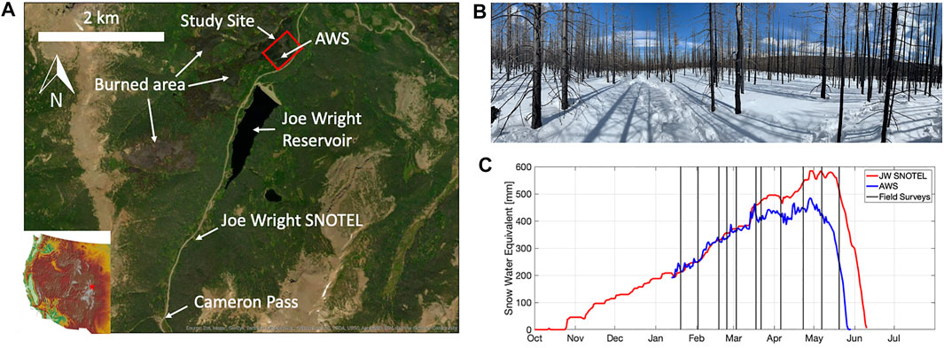
FIGURE 1. (A) Location of the study site and other features in north central Colorado. (B) Photograph of the study site. (C) Snow water equivalent at the Joe Wright SNOTEL station and automatic weather station (AWS) during winter 2020–21. The black vertical lines indicate the GPR and SfM survey dates.

During the 2020–21 winter season, ∼590 mm of SWE accumulated at the Joe Wright SNOTEL station, located 3.8 km southwest of the field site, and an estimated 490 mm of SWE accumulated at an automatic weather station (AWS) within the study site (Figure 1). The SNOTEL station is located outside of the Cameron Peak burn area, while the AWS was installed in the burn area post-fire. SWE at the SNOTEL station is measured directly using a snow pillow equipped with a Sensotec pressure transducer. SWE at the AWS was estimated by combining snow depths measured with a Campbell Scientific SR50A sonic sensor and snow density measured by the SNOTEL station. The GPR/SfM surveys, which extended from mid-January to late May, captured nearly 300 mm of SWE accumulation.

Methods

Observations

Snowpit and Probe Observations

Field observations occurred weekly to biweekly from mid-January until snow disappearance in late May. Snowpit observations were collected centrally within the study plot, with the pit location migrating several meters through time to ensure undisturbed snow was being sampled. For each pit, snow temperature was measured at the snow surface shaded by a shovel blade and then at even 10 cm depths above ground using a Taylor digital thermometer ($\pm$ 0.5°C accuracy). Snow density was measured with a 1,000 cc wedge cutter in duplicate at 10 cm vertical increments along the snowpit face and weighed on a digital scale ($\pm$ 1 g accuracy). A third measurement was made if the first two differed by greater than 20%. Additionally, duplicate permittivity observations were collected at 10 cm vertical increments using an A2 WISe permittivity sensor for nine of the eleven survey dates (the sensor malfunctioned on February 18 and 24). A triplicate was measured if the first two observations were substantially different from each other (e.g., a difference of 0.4 relative permittivity or ∼20%), which only occurred during the May 7 survey. For comparison to the GPR-SfM derived permittivities and densities, we calculated column-averaged values from the mean of the discrete increment observations, after removing the outlier for any observations made in triplicate.

We collected snow depth observations using an aluminum incremented probe ($\pm$ 1 cm resolution) at ∼10 m spacing along a ∼150 m transect across the study plot. The exact probe locations varied between surveys, but individual probe observations were geolocated with a Juniper Systems Geode GNSS receiver (<30 cm horizontal accuracy) mounted on the top of the snow probe. Probe observations that were suspected to have hit a downed tree were removed (4% of total number of observations) prior to comparison with SfM snow depths.

Ground-Penetrating Radar Observations

Ground-penetrating radar surveys were collected using a Sensors and Software PulseEKKO Pro system and two common-offset 1 GHz antennas in broadside orientation with a constant offset of 15 cm. Traces were collected every 0.1 s with a sample rate of 0.1 ns. The antennas were mounted in a plastic sled that was towed on the snow surface behind a technician and offset laterally by ∼50–100 cm to ensure undisturbed snow beneath the radar sled. GPR traces were geolocated using a Emlid RS2 GNSS receiver mounted in the radar sled. The trace positions were post-processed using a second Emlid RS2 GNSS receiver mounted at a fixed location between surveys using RTKLib (version 2.4.3; Takasu and Yasuda, 2009). The final positions have a manufacturer reported horizontal and vertical accuracy of 5 and 10 mm.

Radargrams were processed in ReflexW (Sandmeier geophysical research, 2022) by applying a trace-varying time zero correction, dewow filter, and a background removal 2D filter to enhance the ground reflector. The time zero correction was determined automatically by identifying the first positive reflection for each trace, which were then subsequently smoothed along profile with a 50 trace median filter. The trace spacing was resampled to the mean spacing (∼0.1 m) using the previously described GNSS positions. The twt of the ground reflector was semi-automatically picked using a phase-following algorithm and further refined via manual interpretation (Figure 2).

FIGURE 2

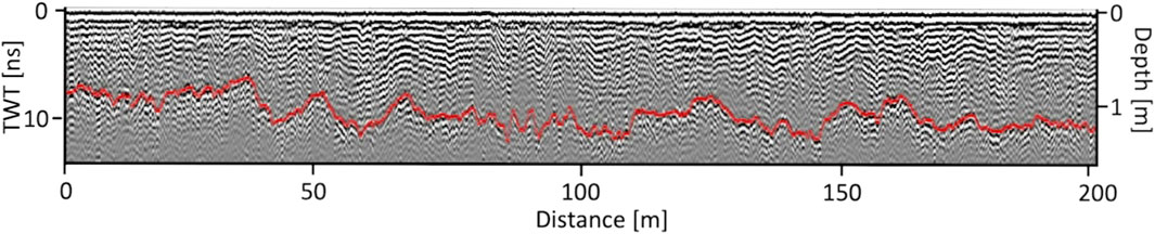
FIGURE 2. Example radargram from 6 April 2021. The semi-automatically picked snow-ground reflector is indicated by the red line. The depth axis is based on an assumed radar velocity of 0.23 m ns⁻¹.

UAV flights and Processing

On twelve dates during the study period, UAV flights were conducted using a DJI Mavic 2 Pro drone in a predetermined double grid flight pattern programmed using Pix4D Capture (Pix4D, 2022). The first flight occurred at ∼60 m above ground level (AGL) with a nadir camera position, while the second orthogonal flight occurred at 50 m AGL with a 20 degree off nadir camera orientation. In total, ∼400 jpeg images were collected between these two flights and, under normal flight conditions (air temperatures between –10 and 0°C and wind speeds <15 mph), the flights required the cumulative use of two standard capacity (3,850 mAh) batteries.

Eleven ground control points (GCPs) were utilized, consisting of five elevated ∼40 cm wide checkered cross targets mounted on top of fixed 2 m tall t-posts and six distinct locations along the road (typically tar strips intersecting the solid white “fog line” at the road margin; Figure 4L). All eleven GCPs were surveyed once near the end of the season (7 May 2021) using an Emlid RS2 GNSS receiver using a post-processed kinematic workflow. A second Emlid RS2 GNSS receiver served as the base station during this survey (∼2 km away); its position was first post-processed in RTKLib using the closest National Geodetic Survey CORS station (COFC; ∼65 km baseline). For each survey, eight GCPs were used to reference the model and three GCPs were used as checkpoints to evaluate model performance.

The SfM processing was completed in Agisoft Metashape (version 1.6.1; Agisoft, 2022). The photos were aligned with “high” accuracy, utilizing adaptive camera model fitting. After alignment, “Gradual Selection” was used to identify and remove lower quality points using the thresholds suggested by Goetz and Brenning (2019). Filtering consisted of reconstruction uncertainty, projection uncertainty and, after GCP import, reprojection error. After lower quality points were removed, a final camera optimization was performed prior to dense point cloud generation. The resulting Control Point and Check Point Errors are reported in Table 1. The dense point cloud was built at “high” quality using aggressive depth filtering. The ground surface was classified using the “Classify Ground Points” function in Agisoft and the resulting ground points were exported as a ASPRS LAS file in UTM Zone 13N (EPSG: 32613). The point cloud was subsequently imported into ArcGIS Pro (ESRI, 2022), where the points were gridded at 1 m resolution without interpolation. These rasters were subsequently differenced (see below) to calculate snow depths.

TABLE 1

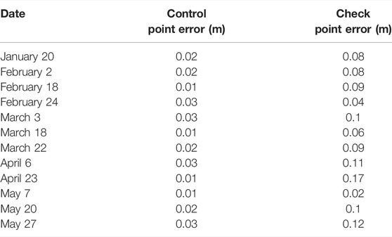
TABLE 1. Control and Check Point Errors for the twelve SfM surveys (eleven snow-on and one snow-off).

Integration of SfM and GPR Observations to Estimate Snow Parameters

Here, we describe 1) how SfM-derived snow depths and GPR-measured twt were combined to estimate radar velocity and relative permittivity for each pixel of overlapping SfM and GPR observations and 2) how relative permittivity outliers were removed in order to calculate a median snow density for each date. This snow density was then applied to all GPR observations on that date to map SWE along the GPR transect. Although not shown, this density value could also be applied to the SfM-derived snow depths to map SWE spatially.

Spatial maps of snow depth were calculated as a DEM of Difference (DoD) by subtracting the snow-off DSM (collected on 27 May 2021) from the snow-on DSM for each prior date. To maximize vertical alignment of the DSMs, we calculated and subsequently removed the median bias of each DoD along a 200 m x ∼8 m wide region of interest along the stable road surface. These values ranged from –0.05 m to 0.09 cm. As the ground surface was not completely snow free on the May 27 survey and a portion of the study plot contains dense canopy (Figure 4L), we created a mask using the high-resolution SfM orthophoto to remove these portions (∼23% of the total area).

GPR twt observations were also gridded to 1 m resolution (with a minimum of 5 traces/pixel) for comparison to the gridded snow depth products by taking the median twt of all traces within that pixel. From these independent observations, radar velocity, $v$, was calculated as:

$v=\frac{SD}{0.5\ast twt}(1)$

where $v$ has units of m ns⁻¹, snow depth, SD, has units of meters, and twt has units of ns. Once the radar velocity was determined for each pixel with coincident observations, the relative dielectric permittivity, $\epsilon$, was calculated as:

$\epsilon ={\left(\frac{c}{v}\right)}^2,(2)$

where c is the speed of light in a vacuum (0.299 m ns⁻¹; Daniels, 2007). To remove outliers and determine a best estimate of $\epsilon$ for each date, we applied two steps: 1) Removed all relative permittivity values less than 1, as those are not physically realistic and 2) removed all relative permittivity values less than the 25% percentile and greater than the 75% percentile (i.e., only include the inner 50% of the distribution). Numerous empirical relationships exist for the conversion of dielectric permittivity to snow density. Previous work (e.g., Di Paolo et al., 2018; Webb et al., 2021) has shown significant scatter between these equations, but for the purposes of this work, we applied two equations: Kovacs et al. (1995) that calculates snow density, $\rho$, from:

$\epsilon ={\left(1+\text{0}\text{.}845\rho \right)}^2.(3)$

and Webb et al. (2021) that calculates snow density from:

$\epsilon =\text{1}+\text{0}\text{.}0014\rho {+2\ast 10}^{-7}{\rho }^2.(4)$

The density units for Eq. 3 are in g cm⁻³ and for Eq. 4 are in kg m⁻³. For the purposes of evaluating the SfM-GPR method, we assume that the snowpack was dry (i.e., LWC = 0). This assumption is valid for the majority of our survey dates, although the snowpack was isothermal on three of the eleven dates. The impact of LWC is further described in the discussion.

Lastly, SWE (presented with units of mm of water equivalent) was calculated as:

$SWE=SD\ast \rho .(5)$

Evaluation of Data Products

The SfM-derived snow depths were evaluated for each date using manual snow depth observations made with the incremented probe. The SfM-GPR derived dielectric permittivities and densities were evaluated with two independent comparisons: 1) A direct comparison to pit-measured permittivities made with the A2 Photonics WISe sensor and 2) a comparison to pit-measured snow densities after the SfM-GPR permittivities were converted to density via empirical relationships. Each of these in situ observations, while made in the same snowpit, are independent from one another. An important distinction, however, is that the value reported from the SfM-GPR analyses are the median value of all values along the ∼150 m transect for that given date, whereas the pit-derived estimates are layer-averaged means from the pit (i.e., a single location proximal to the radar transect). This difference in spatial coverage (transect vs. point) means that there are inherent differences between these estimates due to spatial variations in snow properties, which increased throughout the survey period due to melt.

For each of these comparisons, we report three statistical metrics: 1) The coefficient of determination (r²) from a robust linear regression, 2) the root mean square error (RMSE), and 3) the normalized median absolute deviation (NMAD; Hohlle and Hohle, 2009). The NMAD is comparable to an estimate of the standard deviation that is less sensitive to outliers in the dataset and is calculated as:

$\text{NMAD}=1\text{.}4826\ast \text{median}\left(\left|\Delta h_j-m_{\Delta h}\right|\right)(6)$

Where $\Delta h_j$ are the individual errors and $m_{\Delta h}$ is the median of the errors. A smaller NMAD indicates better agreement between the observations.

Results

Snowpit observations show median snow densities of 270–320 kg m⁻³ between January 20 and March 18 (Figure 3). Snow densities steadily increased after this date, reaching a median density of 430 kg m⁻³ on May 7 and May 20. Median snowpit temperatures ranged between –4.9 and –1.1°C for the survey dates in January through March. For the final four survey dates, median snow temperatures were between –0.2 and 0°C, and on three dates, the snowpack was isothermal over the entire column (Figure 3). Median SfM-derived snow depths increased from 0.65 m on January 20 to a maximum of 1.40 m on March 18, prior to declining to 0.31 m on May 20 (Table 2). The distributed snow depths showed consistent spatial patterns throughout the winter, with regions of lower and higher snow depths persisting through time (Figure 4). SfM-derived snow depths were evaluated with independent measurements of snow depth on each date (Figure 5; Table 2). These comparisons yielded a mean coefficient of determination of 0.67 (range of 0.43–0.81), a mean NMAD of 0.11 m (range of 0.07–0.21 m), and a RMSE of 0.12 m (range of 0.08–0.22 m). There was no significant correlations between these statistical parameters and the median snow depth (r² = 0.09, r² = 0.05, and r² = 0.03, respectively).

FIGURE 3

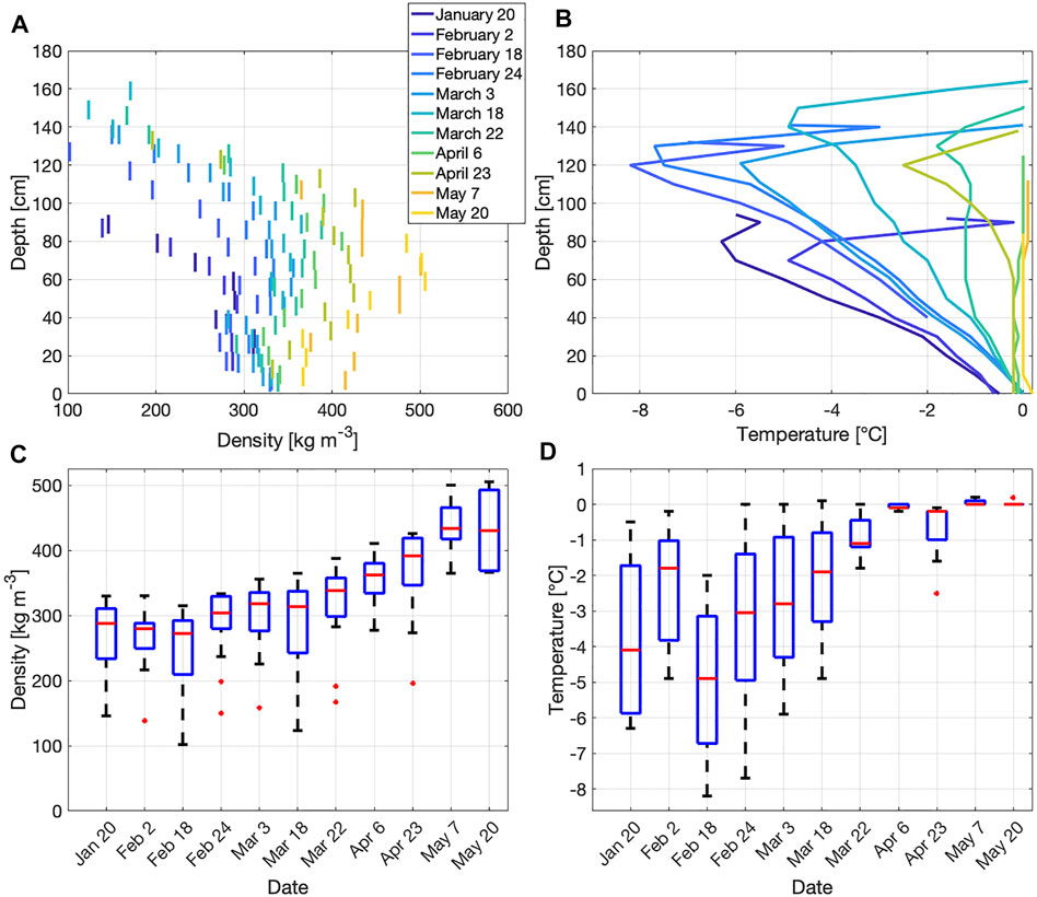
FIGURE 3. (A) Pit-measured snow densities for each layer on each survey date. (B) Pit-measured snow temperatures for each survey date. (C) Boxplots of pit-measured snow densities on each survey date. (D) Boxplots of pit-measured snow temperatures on each survey date.

TABLE 2

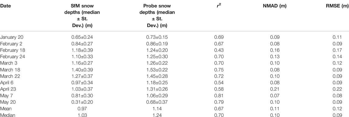
TABLE 2. SfM snow depths (over entire study plot) and probe snow depths (along survey line) and results from statistical comparison.

FIGURE 4

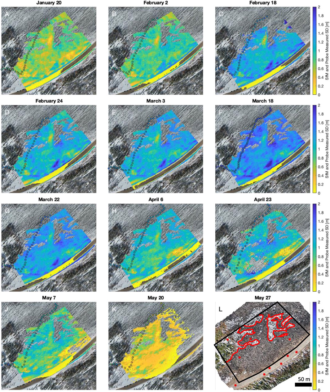
FIGURE 4. (A–K) Plan view of distributed snow depth observations derived from differencing snow-on and snow-off DSMs. The snow depth rasters have been clipped to remove locations where snow persisted in the “snow-off” DSM or significant forest canopy remained. The colored circles in each plot correspond to snow depths measured by a snow probe. (L) Snow-off orthomosaic from 27 May 2021. The black polygon indicates the study regions and the red polygons indicate the masked regions due to remaining snow cover or closed canopy. The red circles indicate locations of GCPs.

FIGURE 5

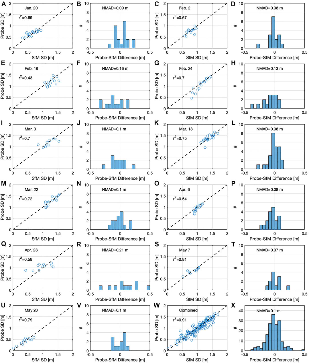
FIGURE 5. (A,C,E,G,I,K,M,O,Q,S,U,W) Scatterplot of probe measured snow depths (SDs) and SfM measured SDs. (B,D,F,H,J,L,N,P,R,T,V,X) Histograms of snow depth differences between the two independent methods. The NMAD is reported for each comparison.

The SfM-GPR derived relative permittivities closely matched the WISe measured permittivities for five of the nine survey dates and largely captured the seasonal evolution of this important parameter (Figure 6A). A comparison of all observations from the winter had a coefficient of determination of 0.67 and NMAD of 0.11 (Figure 6B). Similarly, the seasonal evolution of snow density at the study plot was captured by the SfM-GPR approach, with snow densities below 300 kg m⁻³ until mid to late March, followed by increased densities ranging between 330 and 430 kg m⁻³ in April and May (Figure 6C). For the first six of the eleven survey dates, the SfM-GPR approach, utilizing the Kovacs et al. (1995) equation, underestimated the pit-measured snow densities, with a NMAD of 39 kg m⁻³. For the remaining five surveys, the Kovacs et al. (1995) estimated densities either matched (3) or exceeded (2) the observed snow densities recorded at the SNOTEL station. The Webb et al. (2021) estimated snow densities closely agreed with the SNOTEL densities for four of the first six surveys, but then exceeded these densities for the remaining five surveys (Figure 6C).

FIGURE 6

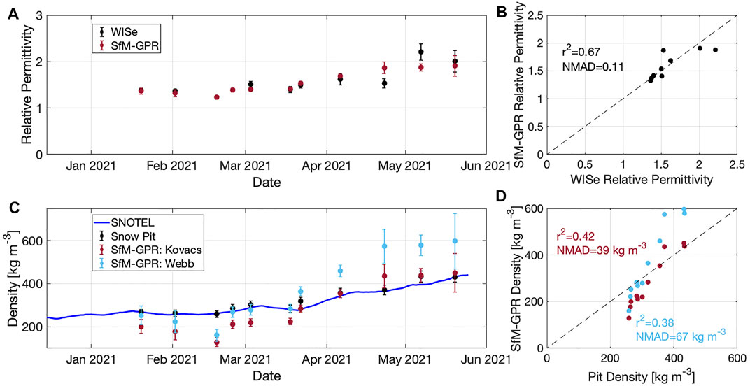
FIGURE 6. (A) Comparison of relative permittivity measured by the A2 Photonics WISe sensor and derived from the SfM-GPR analysis. The error bars for the WISe are based on the standard deviation of the individual layer observations and for the SfM-GPR are the standard deviation of the observations along the transect. (B) Scatterplot of GPR-SfM snow density and pit-measured density. (C) Snow density from the Joe Wright SNOTEL (smoothed with a 14-day window), manual snowpit measurements, and derived from the SfM-GPR analysis. The error bars for the snowpit are $\pm$ 6% of the measured density (Proksch et al., 2016) and for the SfM-GPR are the standard deviation of observations along the transect. (D) Scatterplot of GPR-SfM snow density and pit-measured density using both Kovacs et al. (1995; maroon) and Webb et al. (2021; light blue) empirical relations.

Spatiotemporal patterns in snow depth, based on the SfM surveys, and SWE, calculated using the date specific radar velocities and snow densities, are presented in Figure 7. Given the range in empirically-based density estimates for a given permittivity value, we calculated a mean of both the Kovacs et al. (1995) and Webb et al. (2021) relationships. Snow depth increased from January 20 to March 18, before declining through the end of the season (Figure 7A). In comparison, SWE increased from January 20 to April 23 and then declined during the final two surveys of the season (May 7 and May 20). A similar timing in peak SWE was also observed at the co-located AWS (Figure 1C). The SfM and GPR surveys revealed undulating patterns in snow depth and SWE along the transect that varied on the order of ∼40 cm in depth and ∼100 mm of SWE, respectively (Figure 7). The location of the troughs and peaks remained relatively consistent throughout the winter, likely reflecting patterns of wind redistribution interacting with modest topographic variations, although no simple relationship existed between snow depths and local maxima/minima in elevations (Figure 7A).

FIGURE 7

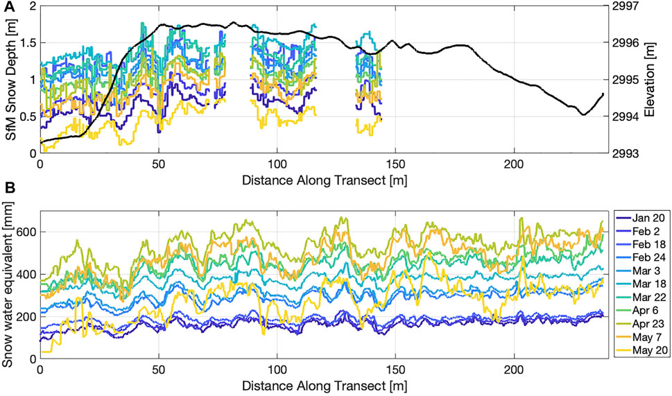
FIGURE 7. (A) SfM-derived snow depths along the GPR-probe transect. The legend in b is applicable to this plot. The snow-off surface elevation is shown in black. (B) Snow water equivalent along the GPR transect for the eleven survey dates.

Uncertainty

We conducted a Monte Carlo analysis to estimate the uncertainty in relative permittivity due to uncertainty in SfM-derived snow depths and GPR twt measurements. SfM snow depth errors can arise from a multitude of sources, including the co-registration of the snow-on and snow-off DSMs and poor SfM reconstructions due to low image contrast/tie point matching. GPR errors can arise from uncertainty in picking the ground reflector in complex terrain (e.g., in the vicinity of downed trees), geolocation errors, or displacement of snow mass by the GPR sled. We present the uncertainty relative to density as it is more applicable to a broader scientific audience than relative permittivity. Previous work has shown significant spread in permittivity-density equations (e.g., Di Paolo et al., 2018; Webb et al., 2021), but for the purposes of this analysis we utilized a single equation to determine the “true” density based on the calculated permittivities, but we acknowledge that the application of this method to derive SWE requires accounting for the potential uncertainty associated with these equations (Di Paolo et al., 2018).

We assume a mean snow depth of 1.0 m and a standard deviation of 0.1 m, which approximates the mean snow depths and SfM-probe NMAD errors during the study period. We assume a mean GPR twt of 8.6 ns and a standard deviation of 0.31 ns Together, the specified depth and twt result in a “true” snow density of 345 kg m⁻³ when the corresponding radar velocity is inverted for density using the Kovacs et al. (1995) equation. The standard deviation of 0.31 ns accounts for two factors: 1) Variability in twt observations within each pixel (calculated as 0.11 ns across all pixels and all survey dates) and 2) a ± 2 samples (0.2 ns) in the measured twt. We assume errors are normally distributed and thus randomly sampled each variable 100,000 times from a normal distribution. The standard deviation of the resulting snow densities, which we use as the uncertainty estimate for our analysis, is 169 kg m⁻³ (Figure 8). The uncertainty in SfM snow depths (0.1 m) alone results in a standard deviation of 159 kg m⁻³, while the uncertainty in GPR twt (0.31 ns) has a standard deviation of 55 kg m⁻³.

FIGURE 8

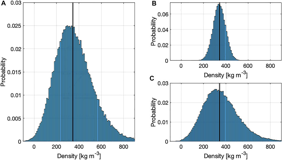
FIGURE 8. (A) Snow densities from a Monte Carlo analysis of uncertainty in SfM-derived snow depths and GPR-measured twt. Black vertical line in all subplots indicates the “true” density of 345 kg m⁻³ (B) Identical analysis but limiting uncertainty to twt. (C) Identical analysis but limiting uncertainty to snow depth.

Discussion

Comparison to Previous Work

The mean statistical parameters reported in this work, r² of 0.67, NMAD of 0.11 m and RMSE of 0.12 m, are comparable to previously reported assessments in the literature. For instance, Eberhard et al. (2021) reported NMAD and RMSEs of 0.11 and 0.16 m for UAS snow depth maps in the Swiss Alps. Bühler et al. (2015) found NMAD and RMSEs of 0.22 and 0.35 m for UAS snow depths compared to manual snow depth measurements. Lastly, Avanzi et al. (2018) reported RMSE of 0.06 and 0.2 m (without and with outliers, respectively) in the second year of their study near Belvedere Glacier in Italy. Yildiz et al. (2021) also coupled SfM and GPR to derive snow density and SWE. This study reports comparable results for independent comparisons of snow depth (correlation = 0.78, RMSE = 9 cm), but lower correlations for snow density when compared to manual snow tube measurements (correlation = 0.14, RMSE = 74 kg m⁻³). Importantly, there are a number of key differences between these studies that are worth noting. First, the study site for Yildiz et al. (2021) included more variable vegetation cover and was more topographically complex, both which could contribute to additional errors in SfM snow depth reconstructions. Secondly, their study presented spatially distributed observations from a single survey date rather than the time series approach presented in this study. We found significant scatter at the individual pixel scale on any given date and thus we focused on calculating a single “best” estimate for each date. Future work could focus on capturing both spatial and temporal variations in density, particularly for study plots where the dynamic range in density on any given date might be larger.

Comparison Between SfM Snow Depths, GPR-SfM Permittivity and Density With Manual Observations

For nine of the eleven survey dates, the NMAD in probe-SfM snow depths were less than 0.15 m and for eight of the survey dates, the NMAD was equal to or less than 0.1 m. For all dates, the probe-SfM snow depth differences were approximately normally distributed around 0 (i.e., the errors were not positively or negatively biased). The largest errors occurred on February 18 and April 23, which had either relatively poor lighting conditions (i.e., flat light and low contrast; Revuelto et al., 2021b), smooth snow textures or intermittent snow showers (April 23), as compared to dates (February 24 and May 7) when the best agreement was evident (Figure 9).

FIGURE 9

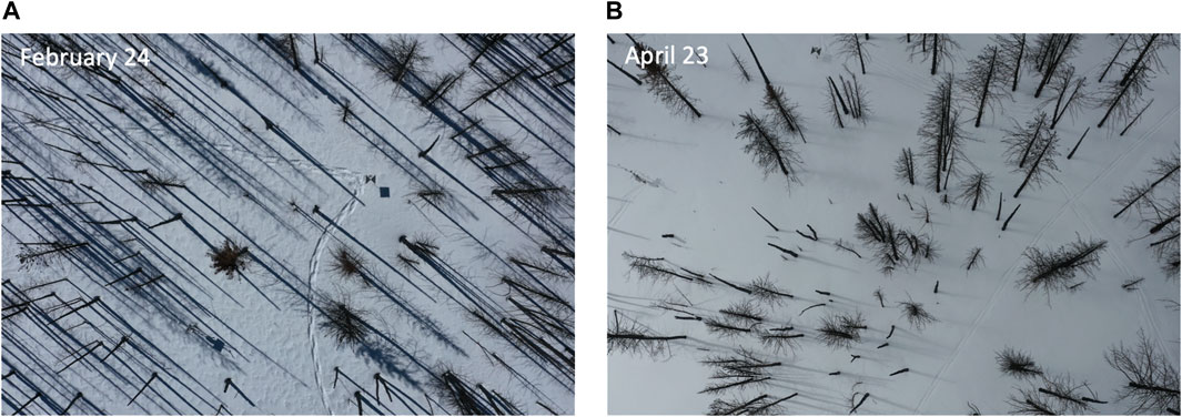
FIGURE 9. Example UAV photographs for two dates ((A) February 24, (B) April 23) showing contrasting lighting conditions and snow surface textures. In (B), the combination of lighting and snow surface conditions likely contributed to the poor agreement with in situ observations.

For the nine survey dates with both WISe and SfM-GPR observations, seven showed close agreement, all of which occurred prior to late April. For the two dates with significant disagreement (April 23 and May 7), the SfM-GPR method first overestimated and then underestimated permittivity relative to the WISe observations. On April 23, the snowpack was nearly isothermal (median layer temperature of –0.2°C) and had multiple ice lenses (<1 cm in thickness, which have a relative dielectric permittivity of ∼3.15; Kovacs et al., 1995) that were difficult to sample with the WISe sensor. By not sampling the ice lenses, the WISe sensor might have underestimated the true permittivity on this date. On May 7, the snowpack was isothermal (median layer temperature of 0°C) and pit observations documented meltwater throughout the snow column. Individual WISe observations were highly variable on this date (>50% of layer observations required a third observation due to substantial differences between the first two observations), indicating high variability within individual layers within the snowpit and likely substantial spatial heterogeneity along the GPR transect. In support of this, we found that the median standard deviation of GPR twt observations within individual 1 m pixels on this date was 0.19 ns, whereas the median for all other dates was 0.11 ns (Figure 10).

FIGURE 10

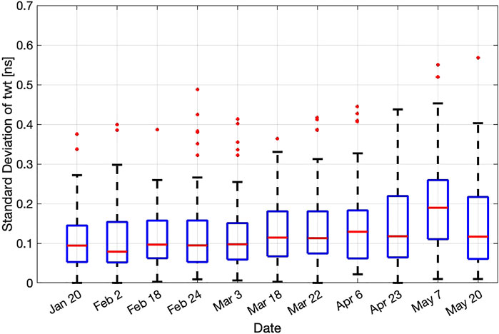
FIGURE 10. Boxplots of the standard deviation of twt within all individual pixel on each survey date.

The NMAD of 39 kg m⁻³ between the SfM-GPR density and pit-measured density is approximately twice as large as a reported maximum uncertainty (e.g., Proksch et al., 2016) on manual density measurements (6% or 18 kg m⁻³ for a density of 300 kg m⁻³), although this difference is likely the result of both real physical differences in density along the GPR transect and errors in each of the methods. We applied two different empirical relationships to convert the derived permittivity to snow density—Webb et al. (2021) showed better agreement to both the pit-measured and SNOTEL-derived density values for permittivities below 1.5 whereas Kovacs et al. (1995) showed better agreement above 1.5 (which corresponds to densities greater than 300 kg m⁻³). This difference potentially reflects the specific snow conditions analyzed during the development of these empirical relations, as the former solely analyzed seasonal snow in Colorado and New Mexico with snow densities below 360 kg m⁻³.

On the last four survey dates, the mean snowpack temperature was $\ge$ –0.6°C, indicating near isothermal or isothermal conditions. The presence of liquid water within the snowpack significantly increases the bulk relative dielectric permittivity (e.g., Bradford et al., 2009; Bonnell et al., 2021; Webb et al., 2021), as water has a relative permittivity of ∼88 and therefore can introduce significant errors in empirical permittivity-density relations that do not account for this component. LWC can be estimated within the snowpack, but it requires three measured parameters: 1) Snow depth, 2) twt, and 3) a dry snow density estimated from snow pit observations. For this study, an explicit goal was to use non-invasive methods (i.e., avoiding snowpits) to estimate snow density and SWE, and thus the last parameter was not available. To explore the corresponding error, we assess the uncertainty associated with the presence of LWC using pit-based calorimeter observations from May 20. The calorimeter observations estimate a LWC of 4.3% on this date (Webb et al., 2021). The presence of this LWC would decrease the radar velocity by ∼18% (from 0.22 m ns⁻¹ to 0.18 m ns⁻¹; Bonnell et al., 2021). On this date, the median SfM measured snow depth was 0.31 m, meaning that the field-measured twt would have increased by ∼23% (from 2.83 to 3.49 ns) due to the presence of the LWC. In addition, the empirically-estimated density (based on the calculated radar velocity and an assumption of dry snow) would increase significantly, from ∼430 to 790 kg m⁻³. However, as shown in Figure 6, this significant overestimate of the true density based on the GPR-SfM integration was not observed. There are a number of potential explanations for this, including 1) the GPR observations were completed before 11 a.m. local, at a time when LWC was at a relative minimum and 2) LWC has been shown to exhibit substantial spatial variability at the scales of meters and thus a single pit based measurement may not be fully representative of a larger area (Griessinger et al., 2018; Webb et al., 2018; Bonnell et al., 2021). In summary, LWC presents a significant and persistent challenge for radar-based methods, particularly in the absence of in situ observations. As such, we recommend that additional considerations of LWC be taken when observations are made when a snowpack is at or near isothermal conditions.

Uncertainty and Lessons Learned

The method presented here is sensitive to uncertainties in both snow depth and GPR-measured twt (Figure 8A). Given reasonable estimates of uncertainty ($\pm$ 0.1 m and $\pm$ 0.31 ns), we find a standard deviation of ∼170 kg m⁻³. When assessed individually, we find that the method is substantially less sensitive to errors in twt (Figure 8B) and more sensitive to errors in snow depth (Figure 8C), resulting in standard deviations in snow density of ∼55 and ∼160 kg m⁻³, respectively. This finding suggests that future improvements in this method focused on reducing the uncertainty in SfM-derived snow depths, perhaps via the use of RTK-enabled UAV platforms, would have the greatest impact. An additional benefit of this approach over others, is that the inverse relationship between snow density and radar velocity (i.e., higher snow density, lower radar velocity), acts to reduce uncertainty in final SWE estimates. In other words, if snow depth is overestimated for a given radar twt, the corresponding velocity will be overestimated, but density and SWE will be underestimated. Alternatively, if snow depth is underestimated for the same twt, the corresponding velocity will be underestimated, but snow density and SWE will be overestimated. While the final errors in SWE are still significant, the inverse relationship between radar velocity and density acts to minimize this error rather than exacerbate it.

The study site was well suited for the application of this method for a multitude of reasons. The area experienced a severe wildfire in the preceding summer, so no ground vegetation was present, thereby removing errors associated with identifying the ground surface in snow-off DSMs and reducing errors associated with correctly identifying/picking the ground surface with the manual snow probe and GPR. The application of this method, along with other depth-based snow remote sensing approaches, would have additional uncertainties where extensive ground vegetation is present. In addition, a plowed road surface paralleled the study site, which allowed for an independent snow-free surface to enable alignment of the respective DSMs on each date. In the absence of this road surface, the corresponding UAV-derived snow depths would have an additional uncertainty of ∼5–10 cm, which would introduce greater uncertainty into the corresponding permittivity and density calculations. Further, the presence of the remaining tree trunks (Figure 9) facilitated tie point identification throughout the full extent of the study area, regardless of the surface snow conditions. In coincident surveys in a nearby meadow devoid of such features, portions of the survey area did not have sufficient texture and/or contrast to produce tie points in the SfM processing. Lastly, the use of static GCPs throughout the survey period greatly improved the efficiency in acquiring UAV imagery on each date, as GCP surveying can be time-consuming and is an additional source of uncertainty.

Conclusion

This study integrated UAV-derived snow depth observations and GPR-measured twt to calculate relative permittivity, snow density and SWE over an entire winter season. SfM-derived snow depths agreed favorably with independent snow depth measurements from manual probing (mean r² = 0.67, NMAD = 0.11 m and RMSE = 0.12). The GPR-SfM derived permittivities and snow densities were additionally compared to independent measurements made in snowpits (relative permittivity: r² = 0.67, NMAD = 0.11 and RMSE = 0.17 and snow density: r² = 0.42, NMAD = 39 kg m⁻³ and RMSE = 68 kg m⁻³). The derived permittivity of individual pixels had significant scatter, so given current technology, this study suggests that this approach is best suited for determining a median permittivity based on a large number of observations along a transect, rather than for individual pixels. The SfM-GPR approach, while sensitive to accurate snow depth observations, is a path forward for non-destructively and efficiently estimating snow density and SWE over intermediate scales and given ongoing development of new technologies in satellite-based snow depth retrievals, this method could be readily expanded to much larger spatial extents.

Data Availability Statement

The original data supporting the conclusions of this article are available at: https://doi.org/10.4211/hs.aa38640675134062aa68df9a6fe92f28.

Author Contributions

DM designed the study, conducted the data integration analyses, and wrote the manuscript. RB processed and picked the GPR data and AO-M processed the UAV imagery. LZ, EB, RB, AO-M, and DM conducted the fieldwork. All authors edited the manuscript.

Conflict of Interest

The authors declare that the research was conducted in the absence of any commercial or financial relationships that could be construed as a potential conflict of interest.

Publisher’s Note

All claims expressed in this article are solely those of the authors and do not necessarily represent those of their affiliated organizations, or those of the publisher, the editors and the reviewers. Any product that may be evaluated in this article, or claim that may be made by its manufacturer, is not guaranteed or endorsed by the publisher.

Acknowledgments

The authors acknowledge the support of the SnowEx leadership team in designing and implementing the SnowEx21 time-series campaign. We thank Megan Mason for her tireless quality control with the SnowEx datasets. We thank Thomas Van Der Weide (BSU) for sharing details on the static GCP design. We thank ZA and AM for their thoughtful comments that have improved the clarity of this manuscript. The authors acknowledge funding support for NASA THP award 80NSSC18K1405. RB acknowledges NASA FINESST award 80NSSC20K1624.

References

Agisoft (2022). Discover Intelligent Photogrammetry with Metashape. Available at: https://www.agisoft.com/(accessed March 30, 2022).

Google Scholar

Avanzi, F., Bianchi, A., Cina, A., De Michele, C., Maschio, P., Pagliari, D., et al. (2018). Centimetric Accuracy in Snow Depth Using Unmanned Aerial System Photogrammetry and a Multistation. Remote Sens. 10 (5), 765–816. doi:10.3390/rs10050765

CrossRef Full Text | Google Scholar

Bonnell, R., McGrath, D., Williams, K., Webb, R., Fassnacht, S. R., and Marshall, H.-P. (2021). Spatiotemporal Variations in Liquid Water Content in a Seasonal Snowpack: Implications for Radar Remote Sensing. Remote Sens. 13, 4223. doi:10.3390/rs13214223

CrossRef Full Text | Google Scholar

Bradford, J. H., Harper, J. T., and Brown, J. (2009). Complex Dielectric Permittivity Measurements from Ground-Penetrating Radar Data to Estimate Snow Liquid Water Content in the Pendular Regime. Water Resour. Res. 45, W08403. doi:10.1029/2008WR007341

CrossRef Full Text | Google Scholar

Bühler, Y., Adams, M. S., Bösch, R., and Stoffel, A. (2016). Mapping Snow Depth in Alpine Terrain with Unmanned Aerial Systems (UASs): Potential and Limitations. Cryosphere 10 (3), 1075–1088. doi:10.5194/tc-10-1075-2016

CrossRef Full Text | Google Scholar

Bühler, Y., Marty, M., Egli, L., Veitinger, J., Jonas, T., Thee, P., et al. (2015). Snow Depth Mapping in High-Alpine Catchments Using Digital Photogrammetry. Cryosphere 9, 229–243. doi:10.5194/tc-9-229-2015

CrossRef Full Text | Google Scholar

Daniels, D. J. (2007). Ground Penetrating Radar. 2nd Edition. London: The Institution of Engineering and Technology.

Google Scholar

Deems, J. S., Painter, T. H., and Finnegan, D. C. (2013). Lidar Measurement of Snow Depth: A Review. J. Glaciol. 59, 467–479. doi:10.3189/2013JoG12J154

CrossRef Full Text | Google Scholar

Deschamps-Berger, C., Gascoin, S., Berthier, E., Deems, J., Gutmann, E., Dehecq, A., et al. (2020). Snow Depth Mapping from Stereo Satellite Imagery in Mountainous Terrain: Evaluation Using Airborne Laser-Scanning Data. Cryosphere 14, 2925–2940. doi:10.5194/tc-14-2925-2020

CrossRef Full Text | Google Scholar

Di Paolo, F., Cosciotti, B., Lauro, S. E., Mattei, E., and Pettinelli, E. (2018). “Dry Snow Permittivity Evaluation from Density: A Critical Review,” in Proceedings of the 2018 17th International Conference on Ground Penetrating Radar (GPR), Rapperswil, Switzerland, 18–21 June 2018, 1–5. doi:10.1109/icgpr.2018.8441610

CrossRef Full Text | Google Scholar

Eberhard, L. A., Sirguey, P., Miller, A., Marty, M., Schindler, K., Stoffel, A., et al. (2021). Intercomparison of Photogrammetric Platforms for Spatially Continuous Snow Depth Mapping. Cryosphere 15, 69–94. doi:10.5194/tc-15-69-2021

CrossRef Full Text | Google Scholar

ESRI (2022). ArcGIS Pro. Available at: https://www.esri.com/en-us/arcgis/products/arcgis-pro/overview (accessed March 30, 2022).

Google Scholar

Goetz, J., and Brenning, A. (2019). Quantifying Uncertainties in Snow Depth Mapping from Structure from Motion Photogrammetry in an Alpine Area. Water Resour. Res. 55, 7772–7783. doi:10.1029/2019WR025251

CrossRef Full Text | Google Scholar

Griessinger, N., Mohr, F., and Jonas, T. (2018). Measuring Snow Ablation Rates in Alpine Terrain with a Mobile Multioffset Ground-Penetrating Radar System. Hydrol. Process. 32 (21), 3272–3282. doi:10.1002/hyp.13259

CrossRef Full Text | Google Scholar

Gubler, H., and Hiller, M. (1984). The Use of Microwave FMCW Radar in Snow and Avalanche Research. Cold Reg. Sci. Technol. 9, 109–119. doi:10.1016/0165-232x(84)90003-x

CrossRef Full Text | Google Scholar

Gubler, H., and Weilenmann, P. (1986). “Seasonal Snow Cover Monitoring Using FMCW Radar,” in A Merging of Theory and Practice: Proceedings of the International Snow Science Workshop, Lake Tahoe, CA, October 22–25, 1986 (Homewood, CA: ISSW Workshop Committee), 87–97.

Google Scholar

Harder, P., Schirmer, M., Pomeroy, J., and Helgason, W. (2016). Accuracy of Snow Depth Estimation in Mountain and Prairie Environments by an Unmanned Aerial Vehicle. Cryosphere 10, 2559–2571. doi:10.5194/tc-10-2559-2016

CrossRef Full Text | Google Scholar

Harpold, A. A., Guo, Q., Molotch, N., Brooks, P. D., Bales, R., Fernandez-Diaz, J. C., et al. (2014). LiDAR-Derived Snowpack Data Sets from Mixed Conifer Forests across the Western United States. Water Resour. Res. 50, 2749–2755. doi:10.1002/2013wr013935

CrossRef Full Text | Google Scholar

Heilig, A., Mitterer, C., Schmid, L., Wever, N., Schweizer, J., Marshall, H. P., et al. (2015). Seasonal and Diurnal Cycles of Liquid Water in Snow-Measurements and Modeling. J. Geophys. Res. Earth Surf. 120, 2139–2154. doi:10.1002/2015jf003593

CrossRef Full Text | Google Scholar

Helfricht, K., Kuhn, M., Keuschnig, M., and Heilig, A. (2014). Lidar Snow Cover Studies on Glaciers in the Ötztal Alps (Austria): Comparison with Snow Depths Calculated from GPR Measurements. Cryosphere 8, 41–57. doi:10.5194/tc-8-41-2014

CrossRef Full Text | Google Scholar

Hohlle, J., and Hohle, M. (2009). Accuracy Assessment of Digital Elevation Models by Means of Robust Statistical Methods. ISPRS J. Photogramm. Remote Sens. 64, 398–406. doi:10.1016/j.isprsjprs.2009.02.003

CrossRef Full Text | Google Scholar

Holbrook, W. S., Miller, S. N., and Provart, M. A. (2016). Estimating Snow Water Equivalent over Long Mountain Transects Using Snowmobile‐ Mounted Ground‐Penetrating Radar. Geophysics 81 (1), WA183–WA193. doi:10.1190/geo2015-0121.1

CrossRef Full Text | Google Scholar

Kovacs, A., Gow, A. J., and Morey, R. M. (1995). The In-Situ Dielectric Constant of Polar Firn Revisited. Cold Regions Sci. Technol. 23, 245–256. doi:10.1016/0165-232x(94)00016-q

CrossRef Full Text | Google Scholar

Li, D., Wrzesien, M. L., Durand, M., Adam, J., and Lettenmaier, D. P. (2017). How Much Runoff Originates as Snow in the Western United States, and How Will that Change in the Future? Geophys. Res. Lett. 44, 6163–6172. doi:10.1002/2017gl073551

CrossRef Full Text | Google Scholar

Lundberg, A., Granlund, N., and Gustafsson, D. (2010). Towards Automated 'Ground Truth' Snow Measurements-A Review of Operational and New Measurement Methods for Sweden, Norway, and Finland. Hydrol. Process. 24, 1955–1970. doi:10.1002/hyp.7658

CrossRef Full Text | Google Scholar

Lundberg, A., and Thunehed, H. (2000). Snow Wetness Influence on Impulse Radar Snow Surveys Theoretical and Laboratory Study. Hydrology Res. 31 (2), 89–106. doi:10.2166/nh.2000.0007

CrossRef Full Text | Google Scholar

Marchand, W.-D., Killingtveit, Å., Wilén, P., and Wikström, P. (2003). Comparison of Ground-Based and Airborne Snow Depth Measurements with Georadar Systems, Case Study. Nord. Hydrol. 34 (5), 427–448. doi:10.2166/nh.2003.0016

CrossRef Full Text | Google Scholar

Marshall, H.-P., and Koh, G. (2008). FMCW Radars for Snow Research. Cold Regions Sci. Technol. 52 (2), 118–131. doi:10.1016/j.coldregions.2007.04.008

CrossRef Full Text | Google Scholar

McCallum, A. (2014). Estimating Snow Density from Dielectric Values Measured Using the Surface Reflection Method. J. Hydrology 53 (2), 179–183.

Google Scholar

McGrath, D., Sass, L., O'Neel, S., McNeil, C., Candela, S. G., Baker, E. H., et al. (2018). Interannual Snow Accumulation Variability on Glaciers Derived from Repeat, Spatially Extensive Ground-Penetrating Radar Surveys. Cryosphere 12, 3617–3633. doi:10.5194/tc-12-3617-2018

CrossRef Full Text | Google Scholar

McGrath, D., Webb, R., Shean, D., Bonnell, R., Marshall, H.‐P., Painter, T. H., et al. (2019). Spatially Extensive Ground‐Penetrating Radar Snow Depth Observations during NASA's 2017 SnowEx Campaign: Comparison with In Situ, Airborne, and Satellite Observations. Water Resour. Res. 55, 10026–10036. doi:10.1029/2019wr024907

CrossRef Full Text | Google Scholar

Meehan, T. G., Marshall, H. P., Bradford, J. H., Hawley, R. L., Overly, T. B., Lewis, G., et al. (2021). Reconstruction of Historical Surface Mass Balance, 1984-2017 from GreenTrACS Multi-Offset Ground-Penetrating Radar. J. Glaciol. 67 (262), 219–228. doi:10.1017/jog.2020.91

CrossRef Full Text | Google Scholar

Mote, P. W., Li, S., Lettenmaier, D. P., Xiao, M., and Engel, R. (2018). Dramatic Declines in Snowpack in the Western US. NPJ Clim. Atmos. Sci. 1 (1), 1–6. doi:10.1038/s41612-018-0012-1

CrossRef Full Text | Google Scholar

Painter, T. H., Berisford, D. F., Boardman, J. W., Bormann, K. J., Deems, J. S., Gehrke, F., et al. (2016). The Airborne Snow Observatory: Fusion of Scanning Lidar, Imaging Spectrometer, and Physically-Based Modeling for Mapping Snow Water Equivalent and Snow Albedo. Remote Sens. Environ. 184, 139–152. doi:10.1016/j.rse.2016.06.018

CrossRef Full Text | Google Scholar

Pix4D (2022). Pix4D Capture. Available at: https://www.pix4d.com/product/pix4dcapture (accessed March 30, 2022).

Google Scholar

Proksch, M., Rutter, N., Fierz, C., and Schneebeli, M. (2016). Intercomparison of Snow Density Measurements: Bias, Precision, and Vertical Resolution. Cryosphere 10, 371–384. doi:10.5194/tc-10-371-2016

CrossRef Full Text | Google Scholar

Raleigh, M. S., and Small, E. E. (2017). Snowpack Density Modeling Is the Primary Source of Uncertainty When Mapping Basin-Wide SWE with Lidar. Geophys. Res. Lett. 44, 3700–3709. doi:10.1002/2016gl071999

CrossRef Full Text | Google Scholar

Revuelto, J., Alonso-Gonzalez, E., Vidaller-Gayan, I., Lacroix, E., Izagirre, E., Rodríguez-López, G., et al. (2021a). Intercomparison of UAV Platforms for Mapping Snow Depth Distribution in Complex Alpine Terrain. Cold Regions Sci. Technol. 190, 103344. doi:10.1016/j.coldregions.2021.103344

CrossRef Full Text | Google Scholar

Revuelto, J., López‐Moreno, J. I., and Alonso‐González, E. (2021b). Light and Shadow in Mapping Alpine Snowpack with Unmanned Aerial Vehicles in the Absence of Ground Control Points. Water Resour. Res. 57, e2020WR028980. doi:10.1029/2020WR028980

CrossRef Full Text | Google Scholar

Roth, K., Schulin, R., Flühler, H., and Attinger, W. (1990). Calibration of Time Domain Reflectometry for Water Content Measurement Using a Composite Dielectric Approach. Water Resour. Res. 26 (10), 2267–2273. doi:10.1029/WR026i010p02267

CrossRef Full Text | Google Scholar

Sand, K., and Bruland, O. (1998). Application of Georadar for Snow Cover Surveying. Nord. Hydrol. 29 (4/5), 361–370. doi:10.2166/nh.1998.0026

CrossRef Full Text | Google Scholar

Sandmeier geophysical research (2022). Sandmeier Geophysical Research. Available at: https://www.sandmeier-geo.de/index.html (accessed March 30, 2022).

Google Scholar

Schmid, L., Heilig, A., Mitterer, C., Schweizer, J., Maurer, H., Okorn, R., et al. (2014). Continuous Snowpack Monitoring Using Upward-Looking Ground-Penetrating Radar Technology. J. Glaciol. 60 (221), 509–525. doi:10.3189/2014JoG13J084

CrossRef Full Text | Google Scholar

Shean, D. E., Alexandrov, O., Moratto, Z. M., Smith, B. E., Joughin, I. R., Porter, C., et al. (2016). An Automated, Open-Source Pipeline for Mass Production of Digital Elevation Models (DEMs) from Very-High-Resolution Commercial Stereo Satellite Imagery. ISPRS J. Photogrammetry Remote Sens. 116, 101–117. doi:10.1016/j.isprsjprs.2016.03.012

CrossRef Full Text | Google Scholar

Siirila-Woodburn, E. R., Rhoades, A. M., Hatchett, B. J., Huning, L. S., Szinai, J., Tague, C., et al. (2021). A Low-To-No Snow Future and its Impacts on Water Resources in the Western United States. Nat. Rev. Earth Environ. 2, 800–819. doi:10.1038/s43017-021-00219-y

CrossRef Full Text | Google Scholar

Sturm, M., Taras, B., Liston, G. E., Derksen, C., Jonas, T., and Lea, J. (2010). Estimating Snow Water Equivalent Using Snow Depth Data and Climate Classes. J. Hydrometeorol. 11, 1380–1394. doi:10.1175/2010JHM1202.1

CrossRef Full Text | Google Scholar

Takasu, T., and Yasuda, A. (2009). “Development of the Low-Cost RTK-GPS Receiver with an Open Source Program Package RTKLIB,” in International Symposium on GPS/GNSS, Jeju, Korea, 4–6 November 2009.

Google Scholar

Vander Jagt, B., Lucieer, A., Wallace, L., Turner, D., and Durand, M. (2015). Snow Depth Retrieval with UAS Using Photogrammetric Techniques. Geosciences 5 (3), 264–285. doi:10.3390/geosciences5030264

CrossRef Full Text | Google Scholar

Webb, R. (2018). Using Ground Penetrating Radar to Assess the Variability of Snow Water Equivalent and Melt in a Mixed Canopy Forest, Northern Colorado. Front. Earth Sci. 11 (3), 482–495. doi:10.1007/s11707-017-0645-0

CrossRef Full Text | Google Scholar

Webb, R. W., Jennings, K. S., Fend, M., and Molotch, N. P. (2018). Combining Ground‐Penetrating Radar with Terrestrial LiDAR Scanning to Estimate the Spatial Distribution of Liquid Water Content in Seasonal Snowpacks. Water Resour. Res. 54 (), 10,339–10,349. doi:10.1029/2018WR022680

CrossRef Full Text | Google Scholar

Webb, R. W., Marziliano, A., McGrath, D., Bonnell, R., Meehan, T. G., Vuyovich, C., et al. (2021). In Situ Determination of Dry and Wet Snow Permittivity: Improving Equations for Low Frequency Radar Applications. Remote Sens. 13, 4617. doi:10.3390/rs13224617

CrossRef Full Text | Google Scholar

Westoby, M. J., Brasington, J., Glasser, N. F., Hambrey, M. J., and Reynolds, J. M. (2012). 'Structure-from-Motion' Photogrammetry: A Low-Cost, Effective Tool for Geoscience Applications. Geomorphology 179, 300–314. doi:10.1016/j.geomorph.2012.08.021

CrossRef Full Text | Google Scholar

Yildiz, S., Akyurek, Z., and Binley, A. (2021). Quantifying Snow Water Equivalent Using Terrestrial Ground Penetrating Radar and Unmanned Aerial Vehicle Photogrammetry. Hydrol. Process. 35 (5), e14190. doi:10.1002/hyp.14190

CrossRef Full Text | Google Scholar