Examining distribution patterns of foraging and non-foraging sperm whales in Hawaiian waters using visual and passive acoustic data

1 Introduction

Cetaceans face a number of threats throughout the world’s oceans, which has resulted in the decline of numerous populations (Magera et al., 2013; Avila et al., 2018). Sperm whales (Physeter macrocephalus) are a cosmopolitan, deep-diving cetacean species listed globally as vulnerable by the IUCN (Taylor et al., 2019) with populations in U.S. waters listed as endangered under the U.S. Endangered Species Act. Following the end of over a century of intensive commercial whaling in 1986, monitoring and assessment of sperm whale populations are essential for guiding management and conservation decisions for their recovery. Using species distribution models (SDMs) to develop a quantitative understanding of the environmental factors influencing sperm whale distributions can lead to a better understanding of their ecology as well as identify important habitats that may overlap with potentially harmful anthropogenic activities (Azzellino et al., 2012; Redfern et al., 2013; Roberts et al., 2016).

Understanding the ecological role of cetaceans relies, in part, on baseline knowledge of their distribution in oceanic waters. SDMs are a common statistical tool that requires ample field observations to precisely estimate these biological patterns, which can provide useful insight for management and conservation strategies (Elith and Leathwick, 2009; Robinson et al., 2017; Melo-Merino et al., 2020). For cetacean SDMs, visual observations are primarily used but recent studies have also incorporated satellite telemetry data (Abecassis et al., 2012; Abrahms et al., 2019) and passive acoustic data (Carlén et al., 2018; Fleming et al., 2018) to increase sample sizes and support more ecologically-based inferences for species that spend the majority of their time underwater.

Multiple studies have used visual sightings and passive acoustic data to study sperm whale distribution patterns with respect to their environment (Jaquet and Whitehead, 1999; Jaquet and Gendron, 2002; Fiori et al., 2014; Fiedler et al., 2018). The unique characteristics of sperm whale clicks make it possible to detect and classify them in the absence of visual observations (Backus and Schevill, 1966). Sperm whales produce several types of clicks depending on their behavior and demographics, which are differentiated by the timing between clicks, or interclick intervals (ICIs), (Whitehead and Weilgart, 1990; Jaquet et al., 2001; Marcoux et al., 2006; Watwood et al., 2006). Codas are repeated stereotyped sequences of clicks lasting approximately 3 s with highly variable group-specific ICIs (Gero et al., 2016; Oliveira et al., 2016; Hersh et al., 2021). Regular clicks (ICI = 0.5–1.5 s) and creaks (ICI <0.5 s) are associated with foraging (Jaquet et al., 2001; Miller et al., 2004; Watwood et al., 2006) while slow clicks (ICI >1.5 s) are produced primarily by male sperm whales (Madsen et al., 2002; Oliveira et al., 2013). The existing knowledge on sperm whale clicks makes it feasible to use passive acoustic data in SDMs to include submerged or diving whales that would otherwise be excluded from the analysis (Gannier and Praca, 2006; Pirotta et al., 2011; Yack et al., 2016; Stanistreet et al., 2018; Diogou et al., 2019).

Sperm whales are one of the most frequently encountered species during visual and acoustic line-transect cetacean surveys in the Hawaiʻi Exclusive Economic Zone (EEZ) (Bradford et al., 2017; Yano et al., 2018). To date, three studies have developed SDMs for sperm whales (and other cetacean species) in the Hawaiʻi EEZ using line-transect sighting data (Forney et al., 2015; Oleson et al., 2015; Becker et al., 2021) but they did not incorporate whale behavior (i.e., foraging or non-foraging) into the analyses. Sampling units in Forney et al. (2015) and Becker et al. (2021) were derived following methods in Becker et al. (2010), which divided the survey effort into 5-km segments and assigned sighting data and environmental predictor values to each segment midpoint along the transect. Models selected static environmental variables (distance to land and latitude) as the important predictors, describing a broad pattern of increasing sperm whale density towards the northwestern region of the Hawaiʻi EEZ (Forney et al., 2015; Becker et al., 2021).

An exploratory study conducted by Oleson et al. (2015) attempted to improve the sperm whale SDMs for the Hawaiʻi EEZ by building models using the same methods as Forney et al. (2015) but also incorporating passive acoustic data collected with towed line arrays of hydrophones. The study included data from a single 2010 survey to compare the predictive power and important variables resulting from SDMs that included only sighting data to SDMs built with only acoustic data. The acoustic-based models selected more dynamic environmental variables (e.g., sea surface temperature and sea surface height), compared to the sighting-based models. However, the accuracy of the acoustic-based models was unclear due to the variability in predictions when modeling different subsets of the acoustic data. It was theorized that by assigning the acoustic data to the segment midpoint of the sampling units along the trackline, the environmental data may have been incorrectly associated with sperm whales acoustically detected up to tens of kilometers from the trackline (Barlow and Taylor, 2005). To overcome this potential issue, a novel method was developed to localize deep-diving cetaceans using towed line array acoustic data (Barkley et al., 2021).

Here, we develop an SDM framework capable of incorporating both sighting and passive acoustic data with a more accurate localization procedure to evaluate distribution patterns of sperm whale groups in the Hawaiʻi EEZ. We base our modeling decisions on known aspects of sperm whale biology and ecology and use the sperm whale click types to differentiate between foraging and non-foraging groups to generate behavior-based SDMs not attempted by prior studies (Forney et al., 2015; Oleson et al., 2015; Becker et al., 2021). We hypothesize that foraging whales occur primarily in deep, more productive offshore waters where they may be more likely to encounter prey compared to non-foraging whales. This research contributes new information about the relationship between sperm whale distribution and environmental features of the Hawaiʻi EEZ, develops new techniques to incorporate visual and passive acoustic data into SDMs, and leverages behavioral information from the acoustic data to examine the habitat preferences between foraging and non-foraging sperm whale groups.

2 Methods

2.1 Data collection and processing

Observational data were collected within the Hawaiʻi EEZ by the National Oceanic and Atmospheric Administration’s (NOAA) Pacific Islands Fisheries Science Center (PIFSC) during cetacean and ecosystem assessment line-transect surveys conducted in 2010, 2013, 2016, and 2017. All surveys followed systematic line-transect sampling protocols described in detail in Yano et al. (2018). Briefly, three observers rotated through three positions searching for cetaceans during daylight hours. Observers along the port and starboard sides used 25 × 150 mounted binoculars while a center observer searched with 7 × 50 binoculars and unaided eyes. If animals were seen within 5.6 km (3 nmi) of the trackline, observers would direct the ship to turn towards the group for species identification and group size estimates.

Continuous acoustic recordings were simultaneously collected using a towed line array of hydrophones. Array configuration varied between surveys, but all arrays contained 4–hydrophones capable of recording frequencies between at least 2–40 kHz. Detailed specifications of passive acoustic arrays and equipment are included in Table 1. Two acousticians aurally and visually monitored the real-time recordings for all cetacean species during daylight hours. A suite of software enabled acousticians to detect and localize vocalizing cetacean groups using 2D target motion analysis (TMA) (ISHMAEL, Mellinger, 2002; PAMGuard, Gillespie et al., 2008). Resulting location estimates were left/right ambiguous due to the linear array design and limitations of 2D TMA. However, the left/right ambiguity was resolved for some localized groups by turning the ship. For each acoustic encounter, or acoustically detected cetacean group, acousticians documented the timestamp of the ship’s trackline location upon first and last detection, the types of vocalizations recorded, the estimated perpendicular distances, and species classification when possible.

TABLE 1

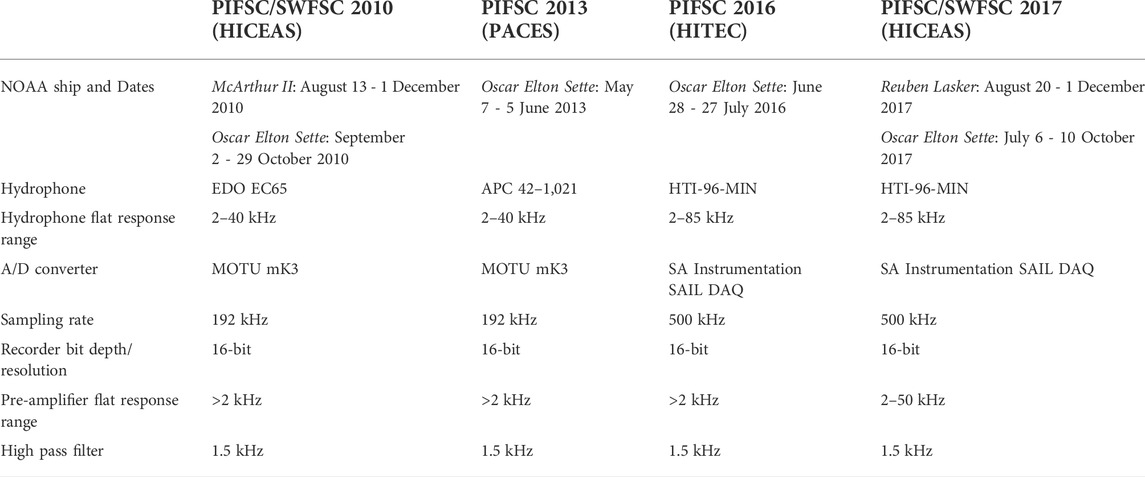
TABLE 1. Details and specifications of the towed line arrays and equipment used for collecting passive acoustic monitoring data during four line-transect surveys conducted in the Hawaiian archipelago.

When sperm whales were visually sighted or acoustically detected based on their recognizable broadband, low frequency (2–15 kHz) echolocation clicks (Backus and Schevill, 1966), each team initiated a specific data collection protocol to reduce bias in visual abundance estimates and collect the necessary information for post-survey acoustic data analyses. Details about the visual and acoustic sperm whale protocols are found in Yano et al. (2018). Briefly, if whales were first visually observed within 5.6 km, at least 70 min were spent counting the number of whales within a group to account for asynchronous dive behavior. If sperm whales were first acoustically detected without corresponding visual observations, the whales were tracked and localized until they passed 90 of the towed array. If the resulting acoustic localization occurred within 5.6 km of the trackline, then the ship was directed towards the whales to attempt visual group size estimates. Whale groups detected beyond 5.6 km by either method were not pursued due to the time needed to divert so far from the trackline, and because groups near this distance are so infrequently sighted that the effective strip width derived for the visual survey is well within this distance (Buckland et al., 2001; Thomas et al., 2006).

2.2 Model data set

All sperm whale acoustic encounters included in the model data set were validated for the presence of echolocation clicks by visually and aurally examining spectrograms of the acoustic data at the time of each encounter using Raven Pro (2048 FFT, Hann window, 50% overlap, version 1.5; Bioacoustics Research Program, 2017). The types of echolocation clicks present in each encounter were determined by ICI measurements. Acoustic encounters that included foraging clicks (i.e., regular clicks or creaks) were labeled as “foraging” groups but could also include other click types. Groups that did not produce foraging clicks during the acoustic encounter were labeled as “non-foraging” and included social groups producing codas and/or male sperm whales producing slow clicks. The term “non-foraging” does not imply fasting but indicates that we did not acoustically detect foraging clicks for the duration of the acoustic encounter and presumed that these groups foraged at other times.

Model data sets for the foraging and non-foraging sperm whale groups included three types of encounters: an acoustic encounter with a concurrent visual sighting (i.e., sighted acoustic), a trackline acoustic encounter, and a localized acoustic encounter. The encounter type dictated which location of the sperm whale group was included in the model data set. For sighted acoustic encounters, we included the location documented by the visual observers. Trackline acoustic encounters included the ship’s location on the trackline at the time of first detection of sperm whales since some groups could not be localized for various reasons (e.g., the whales stopped vocalizing, the ship prematurely turned towards another sighting, or equipment malfunction), but still provided behavioral information to the SDMs.

All localized acoustic encounters were reanalyzed using the model-based localization algorithm described in Barkley et al. (2021) to incorporate more accurate group locations and distance estimates into the modeling data sets. Many of the localized acoustic encounters were left/right ambiguous due to the linear array design and lack of deviation in the ship’s course during the encounter. Since only one location could be included in the model data set, we configured SDMs that used only the left locations, only the right locations, and a random selection of left or right locations to evaluate differences in model results. Results were similar between SDMs (Table 2) supporting the use of a random selection of the left and right locations in the foraging and non-foraging SDMs.

TABLE 2

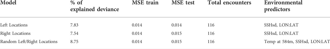
TABLE 2. Percentage of explained deviance, mean squared errors, total encounters, and selected environmental predictors for models comparing data from left and right locations of localized acoustic encounters.

2.3 Model configuration

Each SDM included data collected when visual observers and acousticians were simultaneously on effort actively monitoring for whales while the ship traveled straight to ensure the integrity of acoustic localization results. We used the R programming language (version 4.0.2; R Core Team, 2020) and applied the straightPath function in the ‘PAMmisc’ R package (version 1.6.0; Sakai, 2020) to calculate all straight sections of trackline using the ship’s GPS and heading data. The function compared the ship’s average heading from a 2-min period with the average heading from the previous 8 min. A turn was indicated if the difference between the averaged headings exceeded a threshold of 20°. All data points collected during a turn were excluded from the data set.

Since the number of whales could not be estimated from the localized and trackline acoustic encounters, we used the number of sperm whale groups per grid cell as the unit of the response variable. A gridding method was developed to account for the varying amount of effort occurring throughout each survey. We used customized R functions to overlay grids across the study area and computed an acoustic detection function to calculate survey effort in units of area (km²). The detection function described the relationship between the distance and detection probability of sperm whales and consisted of distance estimates from the localized acoustic encounters to account for the maximum estimated sperm whale detection range within the data set (Figure 1). We modeled the detection function using the ‘Distance’ R package (Miller et al., 2019) to fit a half-normal model to a histogram of the acoustic distance estimates. A truncation distance of 16.22 km was used to remove the largest 3% of distances to improve the fit of the half-normal model as well as determine the 16 km × 16 km spatial resolution of the grid cells (i.e., 256 km² grid cells).

FIGURE 1

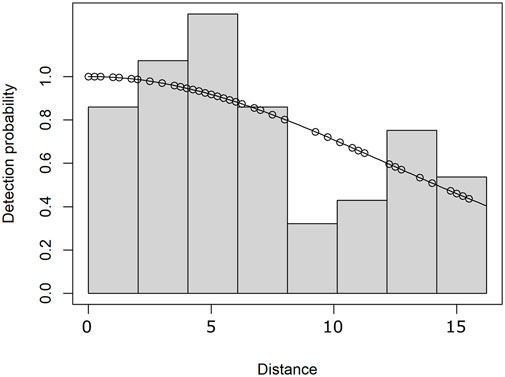
FIGURE 1. Half-normal distribution detection function modeling the detection probability of sperm whales as a function of the distances estimated from the localized acoustic encounters (open circles).

We calculated survey effort per grid cell by summing the product of the survey area and detection probability along all straight trackline segments (Figure 2). The survey area was computed using a series of 1 km × 16.22 km rectangles that extended perpendicularly on either side of the trackline (Figure 2A). These rectangles were then equally divided into 10 pieces that paralleled the trackline. Each piece was extended vertically to the equivalent height of the detection probability function to form a 3D representation of the survey effort (Figure 2B). The volume of each 3D shape was calculated to approximate the integral of the detection function and survey area. The units of effort (km²) are a measure of area; a perfect detection function (i.e., a detection probability of 1.0 across all distances) would result in the exact area of the rectangular survey areas. Only grid cells containing survey effort were included in the models as an offset. The centroids of each grid cell with effort were computed using the ‘sf’ package in R (Pebesma, 2018). Centroids were used to associate sperm whale groups with more accurate environmental data.

FIGURE 2

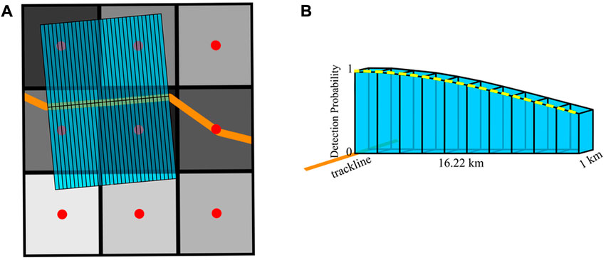
FIGURE 2. Diagram demonstrates the survey effort calculation method. (A) 1 × 16.22 km rectangles (light blue) on the left and right sides of the trackline (orange) represent a sample of survey area computed along a straight trackline segment. Red dots indicate grid centroids. Gray shading in grid cells represents the total amount of effort, which is the cumulative sum of the rectangles, or portion of rectangle, in each cell. Darker gray shades represent more total effort. (B) A 3D representation of a single rectangle with the 10 equal pieces vertically extended to the height of the detection function (yellow dashed line) to calculate the survey effort in each 16 km × 16 km grid cell.

2.3.1 Environmental variables

The environmental predictor variables associated with each grid centroid consisted of static bathymetric features and dynamic remotely sensed variables. The latter were included as indicators of mesoscale oceanographic processes to represent sperm whale habitat and proxies for prey distribution (Table 3). Static variables included seafloor depth, seafloor slope, seafloor aspect, distance to islands, and distance to seamounts. Seafloor bathymetric variables were obtained from the global bathymetry and topography 15 arcsecond data set, SRTM15+ (Tozer et al., 2019). Since aspect and slope were highly uncorrelated between the left and right sides of localized acoustic encounters (Supplementary Figure S1; r = 0, r = 0.27, respectively), they were excluded to minimize uncertainty in the models.

TABLE 3

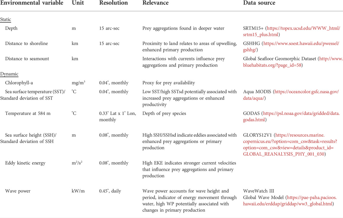
TABLE 3. Candidate environmental variables included as predictors for species distribution models.

The distance to land was obtained from the Global Self-consistent, Hierarchical, High-resolution Geography Database (GSHHG; Wessel and Smith, 1996). This variable addressed the theory that sperm whales are typically found farther offshore, which is also related to depth and suitable prey habitat.

Seamounts are isolated topographic seafloor features taller than 100 m (Staudigel et al., 2010) that aggregate lower trophic level communities, including cephalopods, a main prey item for sperm whales (Clarke et al., 1993; Clarke, 1996; Clarke and Paliza, 2001; Clarke et al., 2007). Since many cetacean species are associated with seamounts (Kaschner, 2007; Wong and Whitehead, 2014) and roughly 600 seamounts exist within the Hawaiian archipelago, we included the distance to seamounts as a predictor variable. Locations of seamounts were extracted from the Seafloor Geomorphic Features Map (Harris et al., 2014). Distances to seamounts were computed with the ‘sp’ and ‘sf’ R packages (Bivand et al., 2013; Pebesma, 2018).

A two-dimensional spatial term (longitude x latitude) was included to explicitly account for geographic effects as well as spatial autocorrelation and integrates over the entire time period of all surveys (Miller et al., 2013; Becker et al., 2018). The inclusion of a spatial term may result in explaining the variation in the data not explained by the other environmental predictors, but it limits the transferability of the models to other study areas.

Remotely sensed dynamic variables included monthly sea surface temperature (SST) and surface chlorophyll-a from the Aqua Moderate Resolution Imaging Spectroradiometer (MODIS) data set. Chlorophyll-a was log-transformed to normalize the variance across the right-skewed observations [log (Chla)]. Sea surface height (SSH), the standard deviation of SSH (SSHsd) and eddy kinetic energy (EKE) were obtained from the global ocean eddy-resolving physical reanalysis data set (GLORYS12V1) generated by the Copernicus Marine Environment Monitoring Service. The EKE is given by:

$EKE=\mathrm{1}/\mathrm{2}\left(U^{\mathrm{2}}+V^{\mathrm{2}}\right)(1)$

where U and V are the zonal and meridional components of geostrophic currents, respectively. The SSH, SSHsd, and EKE act as mesoscale indicators of the ocean vertical structure and reflect gradients in ocean circulation and density structure that may influence the biological responses of lower trophic level organisms (Polovina and Howell, 2005). Wave power (WP) is given by:

$WP=\frac{\rho g^{\mathrm{2}}}{\mathrm{64}\pi }{H}^{\mathrm{2}}{t}_p(2)$

where $\rho$ is the density of seawater (1,024 kg/m³) and g is the acceleration of gravity (9.8 m/s²). Significant wave height, H, and peak wave period, $t_p$, were combined to represent a metric for the size and strength of waves. Monthly temperatures at 584 m were obtained from the Global Ocean Data Assimilation System (GODAS) provided by the NOAA Climate Prediction Center. We selected a depth of 584 m as the best approximate depth of prey habitat from the available options provided by the GODAS data set. This depth corresponded with non-migrant squid species (e.g., Histioteuthis hoylei) that tend to inhabit waters deeper than 400 m and are commonly found in sperm whale stomachs (Young, 1978; Clarke and Young, 1998; Watanabe et al., 2006).

2.3.2 Model parameterization & evaluation

Generalized additive models are a statistical method commonly used in species distribution modeling for their flexibility in fitting complex, nonlinear species-habitat relationships. The data drive the relationships between the response and predictor variables without assuming a specific formula (Guisan et al., 2002). To relate the number of sperm whale groups per grid cell to environmental data, we fitted GAMs using the “mgcv” R package (v. 1.8–31; Wood, 2011) using a Tweedie distribution with a log-link function given the sparse encounter rate data and large numbers of zeros. Model data sets were partitioned into a training and test set with 80% and 20% of the data, respectively. Correlations among the predictor variables were found to be < |0.60|. The natural logarithm of effort was included as an offset variable to account for the variation in effort per grid cell.

Thin-plate regression splines were restricted to three degrees of freedom (12 degrees of freedom for the spatial smoother) to avoid overfitting the non-linear trends and preserve the ecological interpretability of the relationships (Forney, 2000; Ferguson et al., 2006; Roberts et al., 2016). Parameter estimates were optimized using restricted maximum likelihood (Wood, 2011). Model selection was conducted with automatic term selection, determined by the p-values of each predictor (Marra and Wood, 2011). Initial models were built with all potential environmental predictors. Non-significant (α ≥ 0.05) predictors were removed, and models were refit until only significant predictors remained.

SDMs were evaluated using a set of common evaluation metrics calculated on the trained models and the models fitted to the test datasets, including the percentage of explained deviance and the mean squared error (MSE). Partial effects plots were used to visualize the fitted smoothers and interpret the relationship of the selected environmental variables with the response variable.

3 Results

The post-processed acoustic data from the four surveys resulted in 194 total sperm whale encounters (62 sighted acoustic encounters, 74 trackline acoustic encounters, and 58 localized acoustic encounters) (Figure 3). Localized and trackline acoustic encounters accounted for 68% of the total sperm whale groups included in the models. A total of 115 acoustic encounters were identified as foraging groups and 79 were designated as non-foraging groups. The click types present in the foraging and non-foraging groups varied by the encounter type (Figure 4). Sighted acoustic encounters primarily included codas compared to the localized and trackline acoustic encounters, which consisted of mainly foraging and slow clicks. Detection distances ranged from 0.3 to 15.5 km (median = 3.22 km, mean = 4.7 km).

FIGURE 3

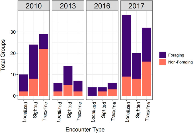
FIGURE 3. Total foraging and non-foraging groups for each encounter type per survey year included in the model data sets.

FIGURE 4

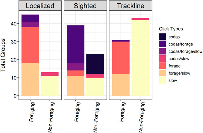
FIGURE 4. Different combinations of click types present in the foraging and non-foraging groups per encounter type (localized, sighted, trackline). “Forage” clicks include regular clicks and/or creaks.

The foraging model had a lower percentage of explained deviance (7.53%) than the non-foraging model (9.21%) with similar MSE values for both models (Table 4). The best-fit foraging model included temperature at 584 m depth (Temp at 584 m °C), the natural log of chlorophyll concentration (log (Chla)), and the 2D spatial smoother (Figure 5). Foraging sperm whale groups peaked in the coolest and warmest deep-water temperatures at 584 m depth but declined with increasing chlorophyll concentration. The 2D smoother for the spatial term showed a majority of foraging sperm whale groups occurring between Laysan Island and Pearl and Hermes Atoll with another cluster of foraging groups associated with the area north of the main Hawaiian Islands.

TABLE 4

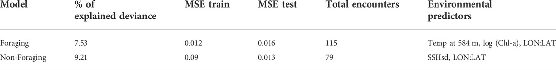
TABLE 4. Percentage of explained deviance, mean squared errors, total encounters, and selected environmental predictors for all models.

FIGURE 5

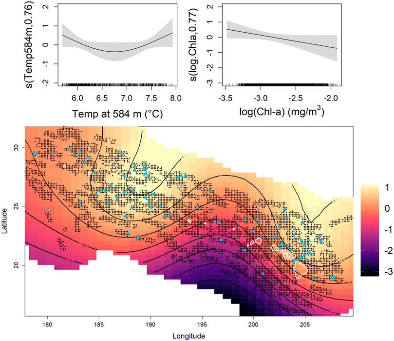
FIGURE 5. Environmental predictors selected for the foraging model included temperature at 584 m, log of chlorophyll-a concentration [log (Chl-a)], and the 2D spatial term (Longitude, Latitude). Light blue dots on the heat map of the spatial term represent encountered foraging sperm whale groups and the black dots indicate surveyed areas included in the model. The black contour lines represent predicted number of whale groups on the link scale and correspond with the color scale, increasing from dark to light colors.

The best-fit model for non-foraging sperm whale groups selected the spatial term and the standard deviation of sea surface height (Figure 6). More non-foraging groups were predicted to be at lower values of SSHsd while the spatial term depicted a relatively uniform spatial distribution of the non-foraging groups across the study area with a moderate increase towards the northwestern region of the Hawaiian archipelago. Overall, no static environmental variables were selected for either model.

FIGURE 6

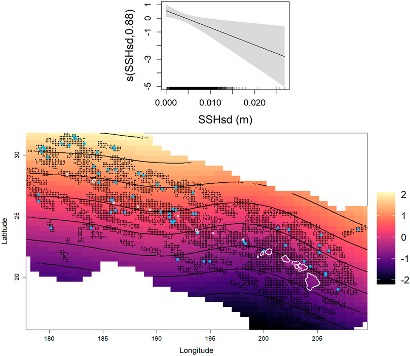
FIGURE 6. Environmental predictors selected for the non-foraging model included the standard deviation of sea surface height and the 2D spatial term (Longitude, Latitude). Light blue dots on the heat map of the spatial term represent all encountered non-foraging sperm whale groups and the black dots indicate all surveyed areas included in the model. The black contour lines represent predicted number of whale groups on the link scale and correspond with the color scale, increasing from dark to light colors.

4 Discussion

Accurately characterizing the distribution of a highly mobile deep-diving marine species is difficult, especially in regions with relatively low animal density and homogeneous environmental conditions. For sperm whales in the Hawaiʻi EEZ, we built SDMs using visual and acoustic data to account for groups at the surface and at depth to improve our understanding of their distribution patterns and help inform population assessments. The addition of acoustic encounters also allowed models to consider foraging behavior and evaluate group demographics. Our findings suggest that sperm whale groups feed at different rates throughout the study area, offering a more direct ecological explanation of sperm whale distribution patterns not always available from visual observations alone.

The Hawaiʻi EEZ study area is influenced by the surrounding oceanographic features of the North Pacific Subtropical Gyre. The northern end of the Northwestern Hawaiian Islands (NWHI) is adjacent to broad frontal zones that promote primary production, which attracts higher trophic level organisms (Seki et al., 2002). The northwesterly flow of the North Hawaiian Ridge Current along the north side of the main Hawaiian Islands (Qiu et al., 1997) may contribute to localized areas of upwelling with enhanced primary production that may lead to patchy aggregations of squids and other sperm whale prey. Eddies and fronts are oceanographic features occurring throughout the year in the study area, indicated by SSH, SST, and their standard deviations, respectively (Qiu, 1999; Firing and Merrifield, 2004; Polovina and Howell, 2005). These mesoscale physical processes enhance nutrient concentrations and primary production in the euphotic zone, eventually benefitting lower trophic levels deeper in the water column. However, the foraging model did not select any predictors related to eddies or fronts, suggesting minimal effects of these features on sperm whales foraging habitat. Only the non-foraging model selected a predictor related to these mesoscale processes, depicting a negative relationship with SSHsd. Since the non-foraging groups primarily included males and social sperm whale groups (identified by slow clicks and codas, respectively), habitat with enhanced prey communities are perhaps not as important compared to the requirements of foraging animals. Lower SSHsd represents less eddy activity and weaker currents, which may be related to less optimal foraging habitat and sufficient conditions for social groups at the time of detection. Overall, these results further support the need to account for different sperm whale behaviors in SDMs (Pirotta et al., 2011; Pace et al., 2018).

Our models included the best available oceanographic data for the study region spanning a 4-year timeframe with no climatological anomalies. Since each survey was conducted at a similar time each year, no significant difference was found in the environmental data across years. However, it only allows us to make general inferences about the physical processes that may be driving the overall distribution of sperm whale groups. A more focused study on the effects of mesoscale physical processes on sperm whale prey would improve our understanding of the potential drivers of sperm whale distribution and whether a better predictor is available to represent this relationship in the models.

We included the temperature at 584 m depth to account for subsurface conditions at an average depth that represented sperm whale prey habitat (Clarke and Young, 1998; Watanabe et al., 2006). The temperature gradient at depth is a persistent characteristic of the North Pacific Subtropical Gyre between depths of ∼250–600 m predicted by GODAS and consists of warmer temperatures west of French Frigate Shoals in the NWHI and cooler temperatures eastward near the main Hawaiian Islands (Wang et al., 2000; Saha et al., 2006). This gradient may be reflected in the correlations between predictions of more foraging sperm whales and the upper and lower ranges of temperature at 584 m, possibly due to a higher abundance of prey influenced by subsurface frontal zones or consistent cold nutrient rich waters. Further research about the prey composition and their depth range is necessary to determine whether a biological explanation exists for the relationship between foraging sperm whales and the temperature at 584 m depth.

Since surface chlorophyll was used to represent prey availability, the explanation for a negative relationship between this variable and foraging groups remains unclear. If results showed a positive relationship, we may infer higher prey abundance in the area from the higher concentration of phytoplankton. Previous work modeled sperm whale occurrence and surface chlorophyll using either time-lagged chlorophyll to account for its incorporation into the food web (Giorli et al., 2016) or tested larger temporal and spatial scales to investigate distribution patterns (Jaquet et al., 1996). One of these methods may shed light on our counterintuitive results, but we suspect that a more indirect link between surface chlorophyll and sperm whale occurrence exists that the SDMs did not capture. Investigation of other environmental variables that better represent additional biological processes at depth may help explain the negative relationship with surface chlorophyll. Finding the appropriate dynamic variables for modeling the distribution of deep-diving species is an ongoing topic of research (Virgili et al., 2022).

Selecting the appropriate spatial resolution is a critical part of configuring any SDM and depends heavily on the research purpose (Redfern et al., 2008). We selected 16 × 16 km grid cells as the most appropriate spatial scale to accommodate several factors, including the acoustic detection distances, the spatial resolution of remotely sensed data sets, and the homogeneous environmental characteristics of the study area. The gridding process included localized acoustic encounters from different towed line arrays to model the detection probability. Ideally, array-specific detection functions would be modeled to account for different array detection ranges (e.g., lower effort values for arrays with shorter detection ranges), but there were insufficient localized encounters per array. Overall, the gridding process introduced more absences in the data set compared to the traditional trackline segment midpoint method of Becker et al. (2010), which, coupled with homogeneous environmental data, likely contributed to poor model performance. However, we now have a modeling strategy that can include different types of sperm whale encounter data and account for varying amounts of effort at any spatial scale. These methods may be more successful when applied to modeling cetacean distributions in more dynamic study areas with greater oceanographic gradients and larger variations in bathymetry.

We initiated this work expecting that localizing acoustic encounters and using environmental data from the animal location (rather than the trackline, as is done in Becker et al. (2010, 2021) would improve upon the relatively imprecise models presented in Becker et al. (2021) and Oleson et al. (2015). Using localized detections following the methods of Barkley et al. (2021), we explored this hypothesis within the modeling process, and concluded that most environmental data associated with the localized acoustic encounters were similar between the left and right location estimates despite their distance from the trackline. Therefore, the uncertainty in model results from Oleson et al. (2015) could not confidently be attributed to using environmental data associated with trackline segments.

In general, it is inherently challenging to model the distribution of sperm whales given their deep-diving behavior and long detection ranges. Even with the additional acoustic encounters and more precise association of environmental data using the gridding method, it is difficult to directly attribute the surface measurements from the environmental data sets to sperm whales that may be influenced by subsurface environmental conditions. The sperm whale SDM presented in Becker et al. (2021) also resulted in relatively low explained deviance and predicted a similar distribution pattern as the foraging model’s spatial term. However, building SDMs that accounted for different encounter types and behavioral groups revealed that certain sperm whale groups may not be well-represented in the current sighting-based sperm whale SDMs for this region. For example, over half of the foraging groups (66%) were acoustically detected without visual confirmation presumably due to their long foraging dives (Figure 4). Additionally, all non-foraging trackline acoustic encounters with slow clicks were missed by visual observers, indicating that small male-only groups are likely under-represented in visual data-only abundance analyses. Further, 61% of the total sighted acoustic encounters included social groups producing codas (Figure 4), groups that are easier to see at the surface. With the behavioral information from passive acoustic data, we are able to identify regions where sperm whales are more likely engaged in foraging and also illustrate that these associations are not well-represented within analyses that rely on visual data only. Further analysis is necessary to evaluate the potential impacts or biases that may emerge from excluding certain sperm whale groups from abundance estimates and population assessments.

This analysis is a step towards developing a better understanding of sperm whale distribution in the Hawaiian archipelago and provides an approach for incorporating behavioral information from passive acoustics into cetacean SDMs. A better ecological understanding of this population may be gained through dedicated surveys in areas of higher sperm whale density that focus on prey sampling and in situ oceanographic measurements of dynamic subsurface variables more related to their foraging habitat at depth. Deploying archival tags to track dive and movement patterns and record acoustic behavior would also provide valuable ecological insight. Future line-transect cetacean surveys should continue to collect visual and passive acoustic data to better understand which types of sperm whale groups are included in population assessments and the regions that are more important for foraging. Continued progress in environmental data acquisition and ocean modeling will also help strengthen the ability of SDMs to incorporate all available observational data to improve our overall understanding of patterns in cetacean distribution and ecology.

Data availability statement

The raw data supporting the conclusion of this article will be made available by the authors, without undue reservation.

Author contributions

YB, EO, and EF conceived the project idea. YB, TS, and EF contributed to the overall analytical approach with TS developing all R functions related to the grid and effort calculations, EF guiding the modeling approach, and YB conducting all analytical steps. All authors contributed to interpreting the results, revising the manuscript, and approving the final version for submission.

Funding

The Funding for passive acoustic data collection during the shipboard cetacean line-transect surveys was provided by Pacific Islands Fisheries Science Center, Southwest Fisheries Science Center, NOAA Fisheries Office of Protected Resources for HICEAS 2010, PIFSC for PACES and HITEC, and PIFSC, OPR, NOAA Fisheries Office of Science and Technology, Chief Naval Operation Environmental Readiness Division and Pacific fleet, and Bureau of Ocean Energy Management for HICEAS 2017. Funding for passive acoustic data analysis was provided by PIFSC and the National Science Foundation Graduate Research Fellowship Program and NOAA award #NA15NMF4520361 (to E.C.F.).

Acknowledgments

This work was made possible by the dedicated officers and crew aboard the R/V Oscar Elton Sette, R/V McArthur II, and R/V Reuben Lasker. We extend our thanks to the scientists who sailed during each survey meticulously collecting the passive acoustic data. Thank you to Margaret McManus and Jeffrey Polovina for reviewing earlier versions of the analysis and manuscript. The authors would also like to thank Devin Johnson for providing an external expert review of our manuscript and the contributions of three outside reviewers.

Conflict of interest

Author TS is employed by Environmental Assessment Services, LLC.

The remaining authors declare that the research was conducted in the absence of any commercial or financial relationships that could be construed as a potential conflict of interest.

Publisher’s note

All claims expressed in this article are solely those of the authors and do not necessarily represent those of their affiliated organizations, or those of the publisher, the editors and the reviewers. Any product that may be evaluated in this article, or claim that may be made by its manufacturer, is not guaranteed or endorsed by the publisher.

Supplementary material

The Supplementary Material for this article can be found online at: https://www.frontiersin.org/articles/10.3389/frsen.2022.940186/full#supplementary-material

References

Abecassis, M., Dewar, H., Hawn, D., and Polovina, J. (2012). Modeling swordfish daytime vertical habitat in the North Pacific Ocean from pop-up archival tags. Mar. Ecol. Prog. Ser. 452, 219–236. doi:10.3354/meps09583

CrossRef Full Text | Google Scholar

Abrahms, B., Welch, H., Brodie, S., Jacox, M. G., Palacios, D. M., Becker, E. A., et al. (2019). Dynamic ensemble models to predict distributions and anthropogenic risk exposure for highly mobile species. Divers. Distrib. (25), 1182–1193. doi:10.1111/ddi.12940

CrossRef Full Text | Google Scholar

Avila, I. C., Kaschner, K., and Dormann, C. F. (2018). Current global risks to marine mammals : Taking stock of the threats. Biol. Conserv. 221, 44. doi:10.1016/j.biocon.2018.02.021

CrossRef Full Text | Google Scholar

Azzellino, A., Panigada, S., Lanfredi, C., Zanardelli, M., Airoldi, S., and Notarbartolo di Sciara, G. (2012). Predictive habitat models for managing marine areas: Spatial and temporal distribution of marine mammals within the Pelagos Sanctuary (Northwestern Mediterranean sea). Ocean Coast. Manag., 67, 63. doi:10.1016/j.ocecoaman.2012.05.024

CrossRef Full Text | Google Scholar

Backus, R. H., and Schevill, W. E. (1966). Physeter clicks, Whales, dolphins and porpoises. University of California Press.

Google Scholar

Barkley, Y. M., Nosal, E.-M., and Oleson, E. M. (2021). Model-based localization of deep-diving cetaceans using towed line array acoustic data. J. Acoust. Soc. Am. 150 (2), 1120–1132. doi:10.1121/10.0005847

PubMed Abstract | CrossRef Full Text | Google Scholar

Barlow, J., and Taylor, B. L. (2005). Estimates of sperm whale abundance in the northeastern temperate pacific from a combined acoustic and visual survey. Mar. Mamm. Sci. 21 (3), 429–445. doi:10.1111/j.1748-7692.2005.tb01242.x

CrossRef Full Text | Google Scholar

Becker, E. A., Forney, K. A., Ferguson, M. C., Foley, D. G., Smith, R. C., Barlow, J., et al. (2010). comparing california current cetacean-habitat models developed using in situ and remotely sensed sea surface temperature data. Mar. Ecol. Prog. Ser. 413, 163–183. doi:10.3354/meps08696

CrossRef Full Text | Google Scholar

Becker, E. A., Forney, K. A., Oleson, E. M., Bradford, A. L., Moore, J. E., and Barlow, J. (2021). Habitat-based density estimates for cetaceans within the waters of the U.S. Exclusive economic zone around the Hawaiian archipelago. NOAA Technical Memorandum. (NMFS-PIFSC-116).

Google Scholar

Becker, E. A., Forney, K. A., Redfern, J. V., Barlow, J., Jacox, M. G., Roberts, J. J., et al. (2018). Predicting cetacean abundance and distribution in a changing climate. Divers. Distrib. 25 (4), 626–643. doi:10.1111/ddi.12867

CrossRef Full Text | Google Scholar

Bioacoustics Research Program (2017). Raven Pro: Interactive sound analysis software. Ithaca, NY: The Cornell Lab of Ornithology

Google Scholar

Bivand, R. S., Pebesma, E., and Gomez-Rubio, V. (2013). Applied spatial data analysis with R. NY: SecondSpringer. https://asdar-book.org/.

Google Scholar

Bradford, A. L., Forney, K. A., Oleson, E. M., and Barlow, J. (2017). Abundance estimates of cetaceans from a line-transect survey within the U.S. Hawaiian islands exclusive economic zone. Fish. Bull. Wash. D. C). 115 (2), 129–142. doi:10.7755/fb.115.2.1

CrossRef Full Text | Google Scholar

Buckland, S. T., Anderson, D. R., Burnham, K. P., Laake, J. L., Borchers, D. L., and Thomas, L. (2001). Introduction to distance sampling estimating abundance of biological populations. New York: Oxford University Press.

Google Scholar

Carlén, I., Thomas, L., Carlström, J., Amundin, M., Teilmann, J., Tregenza, N., et al. (2018). Basin-scale distribution of harbour porpoises in the baltic sea provides basis for effective conservation actions. Biol. Conserv. 226, 42–53. doi:10.1016/j.biocon.2018.06.031

CrossRef Full Text | Google Scholar

Clarke, M. R. (1996). Cephalopods as prey. III. Cetaceans. Philosophical Trans. R. Soc. Lond. B Biol. Sci., 351, 1053

Google Scholar

Clarke, M. R., Martins, H. R., and Pascoe, P. (1993). The diet of sperm whales (physeter macrocephalus linnaeus 1758) off the azores. Philos. Trans. R. Soc. Lond. B Biol. Sci. 339 (1287), 67–82. doi:10.1098/rstb.1993.0005

PubMed Abstract | CrossRef Full Text | Google Scholar

Clarke, M., and Young, R. (1998). Description and analysis of cephalopod beaks from stomachs of six species of odontocete cetaceans stranded on Hawaiian shores. J. Mar. Biol. Assoc. U. K. 78 (02), 623–641.

CrossRef Full Text | Google Scholar

Clarke, R., and Paliza, A. (2001). The food of sperm whales in the Southeast Pacific. Mar. Mamm. Sci. 17 (2), 427–429. doi:10.1111/j.1748-7692.2001.tb01287.x

CrossRef Full Text | Google Scholar

Diogou, N., Palacios, D. M., Nystuen, J. A., Papathanassiou, E., Katsanevakis, S., and Klinck, H. (2019). Sperm whale (Physeter macrocephalus) acoustic ecology at ocean station PAPA in the gulf of alaska – Part 2: Oceanographic drivers of interannual variability. Deep Sea Res. Part I Oceanogr. Res. Pap. 150, 103044. doi:10.1016/j.dsr.2019.05.004

CrossRef Full Text | Google Scholar

Elith, J., and Leathwick, J. R. (2009). Species distribution models: Ecological explanation and prediction across space and time. Annu. Rev. Ecol. Evol. Syst. 40, 677–697. doi:10.1146/annurev.ecolsys.110308.120159

CrossRef Full Text | Google Scholar

Ferguson, M. C., Barlow, J., Reilly, S. B., and Gerrodette, T. (2006). Predicting Cuvier’s (Ziphius cavirostris) and Mesoplodon beaked whale population density from habitat characteristics in the eastern tropical Pacific Ocean. J. Cetacean Res. Manag. 7 (3), 287

Google Scholar

Fiedler, P. C., Redfern, J. V., Forney, K. A., Palacios, D. M., Sheredy, C., Rasmussen, K., et al. (2018). Prediction of large whale distributions: A comparison of presence-absence and presence-only modeling techniques. Front. Mar. Sci. 5, 1–15. doi:10.3389/fmars.2018.00419

PubMed Abstract | CrossRef Full Text | Google Scholar

Fiori, C., Giancardo, L., Aïssi, M., Alessi, J., and Vassallo, P. (2014). Geostatistical modelling of spatial distribution of sperm whales in the Pelagos Sanctuary based on sparse count data and heterogeneous observations. Aquat. Conserv. 24, 41–49. doi:10.1002/aqc.2428

PubMed Abstract | CrossRef Full Text | Google Scholar

Firing, Y. L., and Merrifield, M. A. (2004). Extreme sea level events at hawaii : Influence of mesoscale eddies. Geophys. Res. Lett. 31, 243066–L24314. doi:10.1029/2004gl021539

PubMed Abstract | CrossRef Full Text | Google Scholar

Fleming, A. H., Yack, T., Redfern, J. V., Becker, E. A., Moore, T. J., and Barlow, J. (2018). Combining acoustic and visual detections in habitat models of Dall’s porpoise. Ecol. Model. 384, 198–208. doi:10.1016/j.ecolmodel.2018.06.014

PubMed Abstract | CrossRef Full Text | Google Scholar

Forney, K. A., Becker, E. A., Foley, D. G., Barlow, J., and Oleson, E. M. (2015). Habitat-based models of cetacean density and distribution in the central North Pacific. Endanger. Species Res. 27 (1), 1–20. doi:10.3354/esr00632

PubMed Abstract | CrossRef Full Text | Google Scholar

Forney, K. A. (2000). Environmental models of cetacean abundance: Reducing uncertainty in population trends. Conserv. Biol. 14 (5), 1271–1286. doi:10.1046/j.1523-1739.2000.99412.x

PubMed Abstract | CrossRef Full Text | Google Scholar

Gannier, A., and Praca, E. (2006). SST fronts and the summer sperm whale distribution in the north-west Mediterranean Sea. J. Mar. Biol. Assoc. U. K. 87 (1), 187–193. doi:10.1017/s0025315407054689

PubMed Abstract | CrossRef Full Text | Google Scholar

Gero, S., Whitehead, H., and Rendell, L. (2016). Individual, unit and vocal clan level identity cues in sperm whale codas. R. Soc. Open Sci., 3, 150372. doi:10.1098/rsos.150372

PubMed Abstract | CrossRef Full Text | Google Scholar

Giorli, G., Neuheimer, A., Copeland, A., and Au, W. W. L. (2016). Temporal and spatial variation of beaked and sperm whales foraging activity in Hawai’i, as determined with passive acoustics. J. Acoust. Soc. Am. 140 (4), 2333–2343. doi:10.1121/1.4964105

PubMed Abstract | CrossRef Full Text | Google Scholar

Guisan, A., Edwards, T. C., and Hastie, T. (2002). Generalized linear and generalized additive models in studies of species distributions : Setting the scene. Ecol. Model. 157, 89–100. doi:10.1016/s0304-3800(02)00204-1

CrossRef Full Text | Google Scholar

Harris, P. T., Macmillan-Lawler, M., Rupp, J., and Baker, E. K. (2014). Geomorphology of the oceans. Mar. Geol. 352, 4. doi:10.1016/j.margeo.2014.01.011

CrossRef Full Text | Google Scholar

Hersh, T. A., Gero, S., Rendell, L., and Whitehead, H. (2021). Using identity calls to detect structure in acoustic datasets. Methods Ecol. Evol. 12 (9), 1668–1678. doi:10.1111/2041-210x.13644

CrossRef Full Text | Google Scholar

Jaquet, N., Dawson, S., and Douglas, L. (2001). Vocal behavior of male sperm whales: Why do they click? J. Acoust. Soc. Am. 109 (51), 2254–2259. doi:10.1121/1.1360718

PubMed Abstract | CrossRef Full Text | Google Scholar

Jaquet, N., and Gendron, D. (2002). Distribution and relative abundance of sperm whales in relation to key environmental features, squid landings and the distribution of other cetacean species in the Gulf of California, Mexico. Mar. Biol. 141 (3), 591–601. doi:10.1007/s00227-002-0839-0

CrossRef Full Text | Google Scholar

Jaquet, N., Whitehead, H., and Lewis, M. (1996). Coherence between 19th century sperm whale distributions and satellite- derived pigments in the tropical Pacific. Mar. Ecol. Prog. Ser. 145 (1–3), 1–10. doi:10.3354/meps145001

CrossRef Full Text | Google Scholar

Jaquet, N., and Whitehead, H. (1999). Movements, distribution and feeding success of sperm whales in the Pacific Ocean, over scales of days and tens of kilometers. Aquat. Mamm. 25 (1), 1

Google Scholar

Kaschner, K. (2007). “Air-breathing visitors to seamounts. Section A: Marine mammals,”, Seamounts: Ecology, Fisheries and Conservation. Oxford: Blackwell Publishing Ltd, 230–238.

Google Scholar

Madsen, P. T., Wahlberg, M., and Møhl, B. (2002). Male sperm whale (Physeter macrocephalus) acoustics in a high-latitude habitat: Implications for echolocation and communication. Behav. Ecol. Sociobiol. 53 (1), 31–41. doi:10.1007/s00265-002-0548-1

CrossRef Full Text | Google Scholar

Magera, A. M., Mills Flemming, J. E., Kaschner, K., Christensen, L. B., and Lotze, H. K. (2013). Recovery trends in marine mammal populations. PLoS ONE 8 (10), e77908. doi:10.1371/journal.pone.0077908

PubMed Abstract | CrossRef Full Text | Google Scholar

Marcoux, M., Whitehead, H., and Rendell, L. (2006). Coda vocalizations recorded in breeding areas are almost entirely produced by mature female sperm whales (Physeter macrocephalus). Can. J. Zool. 84, 609–614. doi:10.1139/z06-035

CrossRef Full Text | Google Scholar

Marra, G., and Wood, S. N. (2011). Practical variable selection for generalized additive models. Comput. Statistics Data Analysis 55 (7), 2372–2387. doi:10.1016/j.csda.2011.02.004

CrossRef Full Text | Google Scholar

Melo-Merino, S. M., Reyes-Bonilla, H., and Lira-Noriega, A. (2020). Ecological niche models and species distribution models in marine environments: A literature review and spatial analysis of evidence. Ecol. Model. 415, 108837. doi:10.1016/j.ecolmodel.2019.108837

CrossRef Full Text | Google Scholar

Miller, D. L., Burt, M. L., Rexstad, E. A., and Thomas, L. (2013). Spatial models for distance sampling data : Recent developments and future directions. Methods Ecol. Evol. 4 (11), 1001–1010. doi:10.1111/2041-210x.12105

CrossRef Full Text | Google Scholar

Miller, D. L., Rexstad, E., Thomas, L., Laake, J. L., and Marshall, L. (2019). Distance sampling in R. J. Stat. Softw. 89 (1), 1–28. doi:10.18637/jss.v089.i01

CrossRef Full Text | Google Scholar

Miller, P. J. O., Johnson, M. P., and Tyack, P. L. (2004). Sperm whale behaviour indicates the use of echolocation click buzzes “creaks” in prey capture. Proc. R. Soc. Lond. B 271 (1554), 2239–2247. doi:10.1098/rspb.2004.2863

PubMed Abstract | CrossRef Full Text | Google Scholar

Oleson, E. M., Barlow, J. P., Barkley, Y., Becker, E. A., and Forney, K. A. (2015). Stock Assessment Analytical Methods Annual Report: Incorporating passive acoustic detections into predictive models of cetacean abundance. Honolulu

Google Scholar

Oliveira, C., Wahlberg, M., Johnson, M., Miller, P. J., and Madsen, P. T. (2013). The function of male sperm whale slow clicks in a high latitude habitat: Communication, echolocation, or prey debilitation? J. Acoust. Soc. Am. 133 (5), 3135–3144. doi:10.1121/1.4795798

PubMed Abstract | CrossRef Full Text | Google Scholar

Oliveira, C., Wahlberg, M., Silva, M. A., Johnson, M., Antunes, R., Wisniewska, D. M., et al. (2016). Sperm whale codas may encode individuality as well as clan identity. J. Acoust. Soc. Am. 139 (5), 2860–2869. doi:10.1121/1.4949478

PubMed Abstract | CrossRef Full Text | Google Scholar

Pace, D. S., Arcangeli, A., Mussi, B., Vivaldi, C., Ledon, C., Lagorio, S., et al. (2018). Habitat suitability modeling in different sperm whale social groups. J. Wildl. Manage. 82 (5), 1062–1073. doi:10.1002/jwmg.21453

CrossRef Full Text | Google Scholar

Pebesma, E. (2018). Simple features for R: Standardized support for spatial vector data. R J. 10 (1), 439–446. doi:10.32614/rj-2018-009

CrossRef Full Text | Google Scholar

Pirotta, E., Matthiopoulos, J., MacKenzie, M., Scott-Hayward, L., and Rendell, L. (2011). Modelling sperm whale habitat preference: A novel approach combining transect and follow data. Mar. Ecol. Prog. Ser. 436, 257–272. doi:10.3354/meps09236

CrossRef Full Text | Google Scholar

Clarke, M. R. (2007). “Seamounts and cephalopods,”, Seamounts: Ecology, Fisheries and Conservation. Oxford: Blackwell Publishing Ltd, 207–229.

Google Scholar

Polovina, J. J., and Howell, E. A. (2005). Ecosystem indicators derived from satellite remotely sensed oceanographic data for the North Pacific. ICES J. Mar. Sci. 62 (3), 319–327. doi:10.1016/j.icesjms.2004.07.031

CrossRef Full Text | Google Scholar

Qiu, B., Koh, D. A., Lumpkin, C., and Flament, P. (1997). Existence and formation mechanism of the north Hawaiian Ridge Current, 27. American Meteorological Society, 431

CrossRef Full Text | Google Scholar

Qiu, B. (1999). Seasonal eddy field modulation of the north pacific subtropical countercurrent : TOPEX/poseidon observations and theory. J. Phys. Oceanogr. 29, 2471–2486. doi:10.1175/1520-0485(1999)029<2471:sefmot>2.0.co;2

CrossRef Full Text | Google Scholar

R Core Team (2020). R: A language and environment for statistical computing. Vienna, Austria: R Foundation for Statistical Computing.

Google Scholar

Redfern, J. V., Barlow, J., Bailance, L. T., Gerrodette, T., and Becker, E. A. (2008). Absence of scale dependence in dolphin-habitat models for the eastern tropical Pacific Ocean. Mar. Ecol. Prog. Ser. 363, 1–14. doi:10.3354/meps07495

CrossRef Full Text | Google Scholar

Redfern, J. V., McKenna, M. F., Moore, T. J., Calambokidis, J., Deangelis, M. L., Becker, E. A., et al. (2013). Assessing the risk of ships striking large whales in marine spatial planning. Conserv. Biol. 27 (2), 292–302. doi:10.1111/cobi.12029

PubMed Abstract | CrossRef Full Text | Google Scholar

Roberts, J. J., Best, B. D., Mannocci, L., Fujioka, E., Halpin, P. N., Palka, D. L., et al. (2016). Habitat-based cetacean density models for the U.S. Atlantic and gulf of Mexico’, scientific reports. Sci. Rep. 6 (1), 22615–22712. doi:10.1038/srep22615

PubMed Abstract | CrossRef Full Text | Google Scholar

Robinson, N. M., Nelson, W. A., Costello, M. J., Sutherland, J. E., and Lundquist, C. J. (2017). A systematic review of marine-based Species Distribution Models (SDMs) with recommendations for best practice. Front. Mar. Sci. 4 (421), 1–11. doi:10.3389/fmars.2017.00421

CrossRef Full Text | Google Scholar

Saha, S., Nadiga, S., Thiaw, C., Wang, J., Wang, W., Zhang, Q., et al. (2006). The NCEP climate forecast system. J. Clim. 19 (15), 3483–3517. doi:10.1175/jcli3812.1

CrossRef Full Text | Google Scholar

Sakai, T. (2020). PAMmisc: A collection of miscellaneous functions for passive acoustics. R. package 1, 9.2

Google Scholar

Seki, M. P., Polovina, J. J., Kobayashi, D. R., Robert, R., and Mitchum, G. T. (2002). An oceanographic characterization of swordfish (Xiphias gladius ) longline fishing grounds in the springtime subtropical North Pacific. Fish. Oceanogr. 11 (5), 251–266. doi:10.1046/j.1365-2419.2002.00207.x

CrossRef Full Text | Google Scholar

Stanistreet, J. E., Nowacek, D. P., Bell, J. T., Cholewiak, D. M., Hildebrand, J. A., Hodge, L. E. W., et al. (2018). Spatial and seasonal patterns in acoustic detections of sperm whales physeter macrocephalus along the continental slope in the Western North Atlantic Ocean. Endanger. Species Res. 35, 1–13. doi:10.3354/esr00867

CrossRef Full Text | Google Scholar

Staudigel, H., Koppers, A. A. P., William Lavelle, J., Pitcher, T. J., and Shank, T. M. (2010). Box 1: Defining the word “seamount”. Oceanogr. Wash. D. C). 23 (1), 20–21. doi:10.5670/oceanog.2010.85

CrossRef Full Text | Google Scholar

Taylor, B. L., Baird, R., Barlow, J., Dawson, S. M., Ford, J., Mead, J. G., et al. (2019). Physeter macrocephalus (amendedversion of 2008 assessment). The IUCN Red List of Threatened Species, eT41755A160983555. doi:10.2305/IUCN.UK.2008.RLTS.T41755A160983555.en

CrossRef Full Text | Google Scholar

Thomas, L., Buckland, S. T., Burnham, K. P., Anderson, D. R., Laake, J. L., Borchers, D. L., et al. (2006). Distance sampling’, encyclopedia of environmetrics. Available at: http://onlinelibrary.wiley.com/doi/10.1002/9780470057339.vad033/full.

Google Scholar

Tozer, B., Sandwell, D. T., Smith, W. H. F., Olson, C., Beale, J. R., and Wessel, P. (2019). Global bathymetry and topography at 15 arc sec: SRTM15+. Earth Space Sci. 6 (10), 1847–1864. doi:10.1029/2019ea000658

CrossRef Full Text | Google Scholar

Virgili, A., Teillard, V., Dorémus, G., Dunn, T. E., Laran, S., Lewis, M., et al. (2022). Deep ocean drivers better explain habitat preferences of sperm whales Physeter macrocephalus than beaked whales in the Bay of Biscay. Sci. Rep. 12 (1), 1. doi:10.1038/s41598-022-13546-x

PubMed Abstract | CrossRef Full Text | Google Scholar

Wang, B., Wu, R., and Lukas, R. (2000). Annual adjustment of the thermocline in the tropical Pacific Ocean. J. Clim. 13 (3), 596–616. doi:10.1175/1520-0442(2000)013<0596:aaotti>2.0.co;2

CrossRef Full Text | Google Scholar

Watanabe, H., Kubodera, T., Moku, M., and Kawaguchi, K. (2006). Diel vertical migration of squid in the warm core ring and cold water masses in the transition region of the Western North Pacific. Mar. Ecol. Prog. Ser. 315, 187–197. doi:10.3354/meps315187

CrossRef Full Text | Google Scholar

Watwood, S. L., Miller, P. J. O., Johnson, M., Madsen, P. T., and Tyack, P. L. (2006). Deep-diving foraging behaviour of sperm whales (Physeter macrocephalus). J. Anim. Ecol. 75 (3), 814–825. doi:10.1111/j.1365-2656.2006.01101.x

PubMed Abstract | CrossRef Full Text | Google Scholar

Wessel, P., and Smith, W. H. F. (1996). A global, self-consistent, hierarchical, high-resolution shoreline database. J. Geophys. Res. 101 (4), 8741–8743. doi:10.1029/96jb00104

CrossRef Full Text | Google Scholar

Whitehead, H., and Weilgart, L. (1990). Click rates from sperm whales. J. Acoust. Soc. Am. 87 (4), 1798–1806. doi:10.1121/1.399376

CrossRef Full Text | Google Scholar

Wong, S. N. P., and Whitehead, H. (2014). Seasonal occurrence of sperm whales (Physeter macrocephalus) around Kelvin Seamount in the Sargasso Sea in relation to oceanographic processes. Deep Sea Res. Part I Oceanogr. Res. Pap. 91, 10–16. doi:10.1016/j.dsr.2014.05.001

CrossRef Full Text | Google Scholar

Wood, S. N. (2011). Fast stable restricted maximum likelihood and marginal likelihood estimation of semiparametric generalized linear models. J. R. Stat. Soc. Ser. B 73 (1), 3–36. doi:10.1111/j.1467-9868.2010.00749.x

CrossRef Full Text | Google Scholar

Yack, T. M., Norris, T. N., and Novak, N. (20162016). “Acoustic based habitat Models for sperm Whales in the mariana islands region. Final report. Prepared for U.S. Pacific fleet,” in Submitted to naval facilities engineering command (NAVFAC) pacific, honolulu, Hawaii under contract No. N62742-14-D-1863, issued to ManTech-SRS (Arlington, VA: Prepared by Bio-Waves, Inc).

Google Scholar

Yano, K. M., Oleson, E. M., Keating, J. L., Ballance, L. T., Hill, M. C., Bradford, A. L., et al. (20182017). Cetacean and seabird data collected during the Hawaiian islands cetacean and ecosystem Assessment survey (HICEAS), 72. Honolulu: NOAA Technical Memorandum, 110.

Google Scholar

Young, R. E. (1978). Vertical distribution and photosensitive vesicles of pelagic cephalopods from Hawaiian waters. Fish. Bull. 76 (3), 583.

Google Scholar