Intelligent pointing increases the fraction of cloud-free CO2 and CH4 observations from space

1 Introduction

Multiple satellites now measure atmospheric CO₂ and/or CH₄, with many more missions planned for the future, since these observations enable the quantification of sources and sinks at scales ranging from individual facilities (e.g., Nassar et al., 2017; 2022; Wang et al., 2018) and urban areas (e.g., Wu et al., 2020) to regional and continental scales (e.g., Crowell et al., 2019). Studying these fluxes improves our scientific understanding of processes relevant to climate, while also supporting the emerging capability for policy-relevant emission monitoring in support of climate change mitigation. However, clouds cover approximately 70% of the Earth at any given moment (Stubenrauch et al., 2013) and the retrievals of CO₂ and CH₄ column-averaged dry air mole fractions (XCO₂ and XCH₄) are very sensitive to even small quantities of cloud in the field of view (FOV) (Taylor et al., 2016), primarily because the forward model of the retrieval algorithms lack the detailed physics of clouds due both to its complexity and computational requirements. As a result, most CO₂ and CH₄ satellite missions successfully retrieve XCO₂ or XCH₄ from only a small percentage of raw observations (e.g., ∼7–12% per month for Orbiting Carbon Observatory 2 or OCO-2 version 8, Crisp et al., 2017, 9.5% for OCO-2 v10 Taylor et al., 2023), with the remainder rejected, primarily due to clouds. Discarding this large fraction (∼90%) of data is an inefficient strategy worth reconsidering due to the costs involved in developing, launching and operating the satellites to make these observations.

Japan’s Greenhouse Gases Observing Satellite 2 (GOSAT-2) pioneered Intelligent Pointing (Suto et al., 2021) in which an onboard camera makes real-time measurements that are used to develop cloud masks. GOSAT-2’s greenhouse gas (GHG) instrument, which is equipped with a pointing mechanism, is then directed to point at cloud-free or less cloudy areas to reduce the fraction of observations lost to clouds. GOSAT-2 launched in October 2018 and has since demonstrated that intelligent pointing from Low Earth Orbit (LEO) yields efficiency gains in partially cloudy regions, resulting in a factor of 1.8 more cloud-free observations (Suto et al., 2021).

A geostationary orbit (GEO) is an equatorial orbit with a period that is synchronized with Earth’s rotation providing a vantage point for regional observations with the possibility of a much more rapid revisit rate than LEO. NASA’s Geostationary Carbon Cycle Observatory (GeoCarb) was planned to launch to GEO to observe CO₂, CH₄, CO and Solar Induced Fluorescence (SIF) over the Americas from ∼50°S to 50°N (Moore et al., 2018). Due to cost overruns and technical and logistical issues, GeoCarb was cancelled. The GeoCarb instrument completed integration and following a limited engineering performance test, delivery to NASA is expected in November 2023 for storage and future consideration. GEO GHG mission concepts have also been proposed for Europe (e.g., Burrows et al., 2004; Butz et al., 2015; Butz et al., 2018) and Asia (Rayner et al., 2014), which could together function as a virtual constellation covering Earth’s tropical and mid-latitude land, but viewing geometry limitations prohibit GEO GHG observations beyond ∼50°–55° latitude.

A highly elliptical orbit (HEO) can be used to make rapid revisit “quasi-geostationary” observations over higher latitudes, although at least two satellites are required to cover each circumpolar region. The Arctic Observing Mission (AOM) is a HEO mission concept that is under consideration for implementation by Canada with international partners aiming to launch in the mid-2030s. AOM is an expanded version of the Atmospheric Imaging Mission for Northern Regions (AIM-North, Nassar et al., 2019), adding meteorology and space weather instruments along with GHG and air quality payloads. In early studies (Phase 0), two different spectrometer technologies were considered for AOM GHG observations: a dispersive spectrometer and an imaging Fourier Transform Spectrometer (IFTS). OCO-2 (Crisp et al., 2017), OCO-3 (Eldering et al., 2019), TanSat (Yang et al., 2018), the Tropospheric Monitoring Instrument (TROPOMI, Veefkind et al., 2012), MethaneSat (Staebell et al., 2021), MicroCarb (Pasternak et al., 2016), GeoCarb (Moore et al., 2018), the Global Observing Satellite for Greenhouse gases and Water cycle (GOSAT-GW, Kasahara et al., 2020), Copernicus CO₂ Monitoring Mission (CO2M, Sierk et al., 2021) and CO2Image (Krutz et al., 2022) are examples of satellite missions with dispersive spectrometers for CO₂ or CH₄ observations. GOSAT (Kuze et al., 2009), GOSAT-2 (Suto et al., 2021) and Feng-Yun-3D Greenhouse gas Absorption Spectrometer (GAS) (Bi et al., 2022) are examples of CO₂ or CH₄ missions that use single-element Fourier Transform Spectrometers (FTSs). The AOM baseline plan calls for an IFTS, as formerly proposed for GEO-FTS (Xi et al., 2015). An example of an IFTS already flying in space for a different application is China’s Geostationary Interferometric InfraRed Spectrometer (GIIRS) meteorological instrument, operating in the mid-IR, which will be joined by a European GEO meteorological IFTS in 2024 (MeteoSat Third Generation Infrared Sounder: MTG-IRS) and a U.S. GEO meteorological IFTS in the mid-2030s.

Dispersive spectrometers utilize a 2-dimensional (2D) focal plane array (FPA) detector by allocating one dimension for spectral information and one for spatial information, such that spectra are simultaneously observed for a row of pixels in a duration of seconds or even fractions of a second. In an IFTS, both dimensions of the FPA are used for spatial information, simultaneously observing 2D images with an interferogram for each pixel in which the spectral information is effectively in the time domain and recovered mathematically by applying a Fourier Transform. Thus, an IFTS has the advantage of recording a simultaneous 2D image but obtaining a sufficient signal-to-noise ratio (SNR) requires staring at the same air column and integrating the signal substantially longer than for a dispersive spectrometer. Although this is impractical to do from LEO with a satellite moving at 7 km/s relative to the ground, it enables new possibilities from GEO or HEO.

For GOSAT-2 in LEO, intelligent pointing yields an advantage in partially cloudy situations, but not when the field of regard (FOR) is entirely cloudy or entirely cloud-free since there is no better/worse location to point within the FOR. It is expected that from GEO or HEO, from which nearly the whole Earth disk can be observed, the benefits of an intelligent, cloud-informed pointing approach would be greater than from LEO, as there will likely always be some cloud-free locations within the FOR to observe. Figure 1 shows an orthographic projection of the Earth as could be seen from HEO, depicting the number of cloud-free daylight hours per month in 2015, based on NASA Modern Era Analysis for Research and Applications (MERRA-2, Molod et al., 2015; Gelaro et al., 2017) cloud fraction data discussed in Section 2.2. Excluding dark northern winter months (December, January, February), northern land typically has non-zero values, indicating opportunities for cloud-free viewing, if a satellite can point at those regions at the correct time. GEO and HEO can enable flexible viewing capability to facilitate this strategy, while it is impractical from LEO, especially from a sun-synchronous LEO, where an overpass time is essentially fixed. Methods to exploit the flexible viewing advantage of GEO and HEO in future CO₂ and CH₄ satellites warrant some consideration.

FIGURE 1

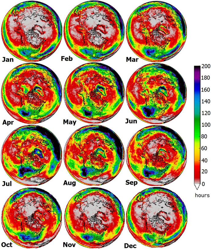
FIGURE 1. Distribution maps of the number of cloud-free daylight hours per month based on NASA MERRA-2 data (0.5° × 0.625°) for 2015.

In this work, intelligent pointing simulations were conducted for dispersive and IFTS instruments in HEO, accounting for how the technologies scan a spatial region in different ways. Section 2 describes our methodology for generating synthetic observations and the assumptions about standard pointing and intelligent pointing. Our simulation results are presented in Section 3 showing significant advantages for intelligent pointing for satellites in HEO from which nearly the whole Earth disk can be observed. The implications of these results including for the design of future satellite constellations for observing CO₂ or CH₄ (Crisp et al., 2018), such as the choice of instrument technology and the use of different orbit classes: LEO, GEO and HEO are discussed in Section 4.

2 Methods

The pointing simulations in this work involved simulating the following factors, described below:

1) Position of the satellite in orbit.

2) Instrument viewing characteristics.

3) Solar illumination and viewing geometry.

4) Land mask.

5) Dynamic cloud fields.

6) Observing strategy for each instrument.

2.1 Orbit

Simulation of GEO is trivial from an orbital perspective, since the satellite is stationary over a certain longitude at the Earth’s equator. Simulation of satellite positions in HEO is more complicated. Here we assume the orbital parameters for a Three Apogee (TAP) orbit as given in Table 1 A figure of this particular orbit and the hourly locations of a satellite in this orbit is available in Nassar et al. (2019). The apogee longitudes of 95°W, 25°E and 145°E are selected for good observational coverage of North America, Europe and Asia, with the complete ground track of this orbit shown in Figure 2. A satellite in this orbit spends most of its time in the northern mid- and high latitudes, in the proximity of the three apogee locations (northernmost points of the ground tracks). Two satellites in this orbit, spaced half the orbital period (∼8 h) apart, but in the same orbital plane, were simulated using NASA’s General Mission Analysis Tool (GMAT, https://software.nasa.gov/software/GSC-17177-1). The GMAT latitude, longitude and altitude for each satellite was written to file at 1-min intervals and we linearly interpolate between these points.

TABLE 1

TABLE 1. Orbital parameters for AOM applied in simulations.

FIGURE 2

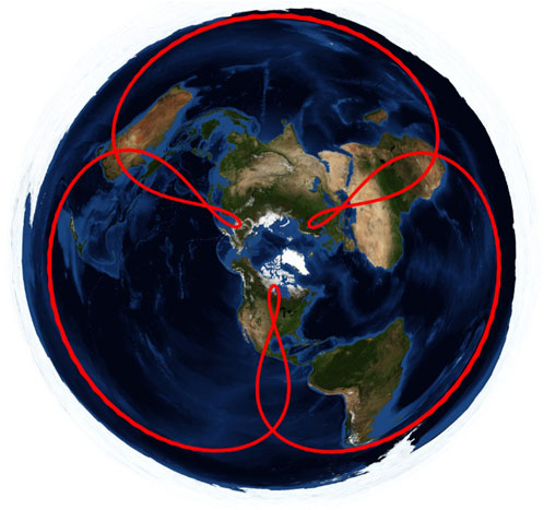
FIGURE 2. Ground track for a Three Apogee (TAP) orbit with e = 0.50 and apogee longitudes of 95°W, 25°E and 145°E.

HEOs exhibit a drift in the right ascension of the ascending node (RAAN or Ω). Calculation of the RAAN rate of change or $\dot{\mathrm{\Omega }}$ is described in Trishchenko and Garand (2011) and Trishchenko et al. (2011) and for our baseline TAP orbit, $\dot{\mathrm{\Omega }}$ = −10.03°/year and the time of apogee changes on a cycle of 355.1 days. An implication of this RAAN drift is that the local time that the satellite reaches apogee also drifts over this cycle. In this work, each HEO satellite is set to reach apogee at exactly local noon on July 25 of the first year in orbit and the date of local noon observation from apogee drifts forward by ∼10 days/year.

2.2 Instrument viewing characteristics, geometry and other considerations

The AOM GHG instrument is an Imaging Fourier Transform Spectrometer (IFTS). Its design is still preliminary and could change prior to eventual launch but the current baseline design has 4 near-infrared - shortwave infrared (NIR-SWIR) bands (Table 2), each with a dedicated focal plane array (FPA). A dispersive spectrometer would use the bands planned for GeoCarb, which they optimized with noise considerations for that instrument type (McGarragh et al., 2023).

TABLE 2

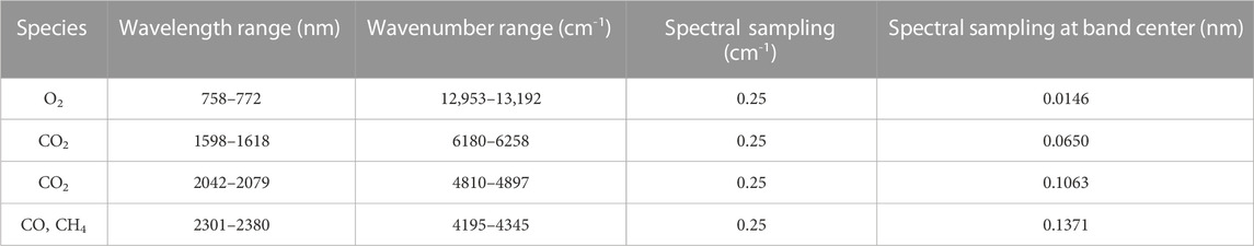
TABLE 2. Spectral bands for the AOM IFTS instrument.

The instrument configurations simulated in this study are shown below in Table 3. For each, the instantaneous field of view (IFOV) of the instrument is given along with the stare time required to integrate for the observation. For the two IFTS configurations, the stare duration is 60 s, in which each observes a 2D image of pixels. For the dispersive spectrometer, which observes a 1D IFOV of pixels, 36 rows are observed over 63 s, which are combined to form a 36 × 480 pixel image, then the instrument is repointed. For the purpose of this study, we refer to each ∼1-min collection as the FOV, acknowledging that this slightly differs from the typical use of the term. Since the number of stares per minute multiplied by the IFOV gives us the FOV, the FOV and IFOV are equal for the IFTS. Combining the integration time and some time for repointing (IFTS: 6 s, dispersive 4 s), 54 FOVs are observed for each instrument per 1-h cycle and the resulting number of raw observations are given in Table 3.

TABLE 3

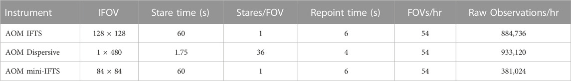
TABLE 3. Instrument observing characteristics.

The nominal pixel size for all instruments compared here is 4 × 4 km², but actual pixel sizes differ for two reasons. Firstly, for either GEO or HEO, off-nadir observations result in pixel growth in one or both dimensions for geometrical reasons. This view zenith angle (VZA, sometimes also called the sensor zenith angle) effect is accounted for in these simulations. Secondly, for HEO, the altitude of the satellite changes throughout an orbit and the instrument’s angular FOV remains constant, without compensating for this effect. So for HEO, the nominal pixel size is obtained at 40,000 km in altitude, while pixels can become much smaller for lower altitudes and up to ∼4.7% larger for higher altitudes near apogee (41,887.7 km). The selection of a 4 × 4 km² pixel threshold was influenced by the study by Hill and Nassar (2019) for potential anthropogenic CO₂ emission quantification applications.

Due to the low shortwave infrared (SWIR) albedo of diffuse reflectance over bodies of water, only observations over land will yield sufficient signal for successful retrievals, unless glint geometry is used. However, glint viewing opportunities from GEO and HEO are very limited, thus are not planned for AOM nor were they planned for GeoCarb. Therefore, a pre-determined scan pattern to cover land within the area of interest is the simplest approach. Figure 3 is an example of an AOM pointing grid, which covers the primary area of interest, which is ice-free land from ∼45 to 80°N, but the grid reaches ∼42°N in eastern North America to include the southernmost portion of Canada. A new HEO pointing grid is defined for each 1-h pointing cycle since the FOV dimensions on the Earth’s surface change due to altitude and VZA as mentioned. Since HEO satellites are in position to observe the area of interest with an adequate VZA for about 2/3 of an orbit, there are 11 1-h cycles during a 16-h orbit. For simplicity, we assume symmetry for cycles 1 and 11, 2 and 10, 3 and 9, etc. (neglecting small changes in satellite longitude) giving 6 unique grids for each apogee for a total of 18.

FIGURE 3

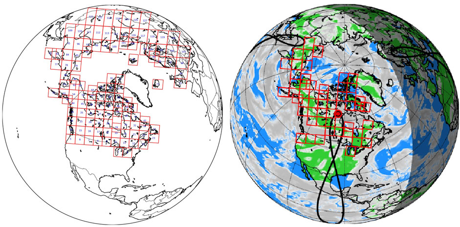
FIGURE 3. Example of an IFTS pointing grid from apogee at 95°W and an example of FOVs selected for cloud avoidance in one viewing cycle (June 2, 22:00 UTC) under an intelligent pointing approach.

A standard step-and-stare pointing approach, as was proposed for GEO-FTS (Xi et al., 2015), would involve pointing at each of the FOV locations in the pointing grid, 125 locations in this example, although even more FOVs are needed for apogees over Eurasia. At 54 stares/h, this would require 2, 3 h to cover, i.e. 2, 3 h revisit period. Depending on the season, some fraction of these FOV locations would be in darkness or at a solar zenith angle (SZA) too large for proper observation. On average, about half the area would be sunlit, although more in the Arctic summer and less in the winter. Excluding the dark areas reduces the summer revisit rate to slightly under 2 h, but excluding areas of thick cloud makes hourly revisit of the less cloudy areas possible over most of the year, an unprecedented revisit rate for greenhouse gas observations from space.

For cloud information to guide pointing decisions, our simulations use cloud fractions from the NASA’s MERRA-2 reanalysis (0.5° × 0.625°, 72 levels, 3-h average, Molod et al., 2015; Gelaro et al., 2017), which are interpolated to hourly. To simplify our simulations, we do not trace the incoming and reflected sunlight through a 3D atmospheric cloud field. Instead, the highest cloud fraction (CF) value for any level is treated as the column value, which is used to make a 2D CF field. To account for the increased impact of clouds for longer paths through the atmosphere, we determine an effective cloud fraction (ECF). To calculate ECF, first we calculate the airmass = 1/cos (SZA) + 1/cos (VZA), which is a minimum of 2 when both SZA = VZA = 0° and a maximum of 7.76 for VZA = 60° (AOM) and SZA = 80°. Then:

$ECF=CF\mathrm{x}airmass/2$

and a certain number observations are assumed to penetrate through the ECF field according to Table 4. To test the realism of this simulated cloud loss method, we applied it to raw OCO-2 observation locations and times and obtained excellent agreement in terms of the total number of post-filtered observations per month and the latitudinal distribution of observations per month (not shown).

TABLE 4

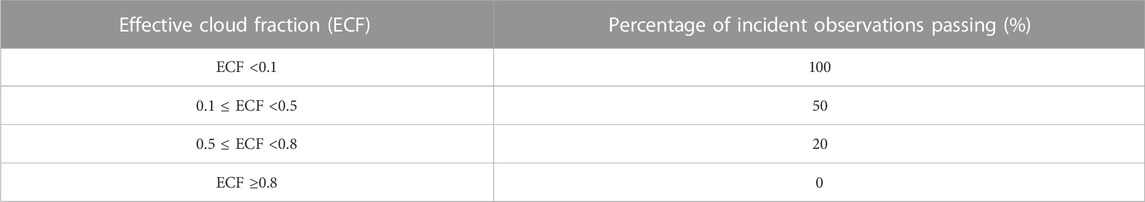
TABLE 4. Percentage of successful observations for different effective cloud fraction ranges.

Based on the location of the satellite in orbit, the VZA to any location within the FOR is also calculated. In this work, only observations with SZA ≤80° and VZA ≤60° over land are accepted. A 0.1° × 0.1° land mask is used to remove observations over the oceans, lakes, and other bodies of water. Old snow and ice also have very low SWIR albedo (e.g., Nassar et al., 2014), so observations over Greenland are essentially excluded, while those over areas of seasonal snow are included, but will have poorer precision than observations over other land cover types. To account for dark surfaces and the spatial distribution of albedo at this wavelength in general, we use Moderate Resolution Imaging Spectroradiometer (MODIS) Level 3 monthly-averaged surface Band 6 albedo (1628–1652 nm, Schaaf and Wang, 2021) and reject observations where this albedo is <0.02. Dense aerosols also result in the loss of observations, but this is typically confined to a much smaller region than clouds. We apply Terra Multi-angle Imaging SpectroRadiometer (MISR) Aerosol Optical Depth (AOD) (Diner et al., 2005) and reject observations where AOD >0.3 (e.g., O’Dell et al., 2012).

2.3 Intelligent pointing vs standard pointing

The AOM IFTS would observe 128 × 128 pixels in 60 s, then requires 6 s to repoint. In standard pointing, the IFTS would point at all sunlit locations in the pointing grid (e.g., Figure 2) then repeat the cycle. For intelligent pointing, a cloud mask would guide the pointing to observe only the clearest regions. This is accomplished by ranking FOVs in the grid with those having low cloud, good solar illumination and a northerly location ranking as a higher observing priority. Using the cloud fractions for each FOV calculated earlier, we define the priority of the FOV related to cloud as follows:

$p_{cloud}=1-\overline{cloudfraction}$

where the overbar represents a mean across all the pixels in the FOV. Thus p_cloud = 0 corresponds to the worst viewing conditions and p_cloud = 1 corresponds to the best. Other priority factors are also normalized to the 0–1 range, with 0 being the worst and 1 the best.

The second priority factor is the airmass, with a lower airmass receiving higher priority. A low airmass corresponds to the pixels of the FOV being less stretched, the Sun being higher in the sky and results in less loss of data due to cloud, so:

$p_{airmass}=\frac{{airmass}_{\mathit{max}}-\overline{airmass}}{{airmass}_{\mathit{max}}-{airmass}_{\mathit{min}}}$

AOM coverage for greenhouse gas observations extends from ∼42 to 80°N, giving some overlap with potential future geostationary coverage; however, high latitudes are still the priority, so we add a priority related to the central latitude $\phi$ of the FOV:

$p_{latitude}=\raisebox{1ex}{$\phi $}\!\left/ \!\raisebox{-1ex}{$90°$}\right.$

The final priority factor relates to the viewing history of the satellite, so that infrequently viewed areas are given a higher priority than areas that have already been viewed frequently. Since the FOV grid changes throughout an orbit, history is recorded on a 5° × 5° latitude/longitude grid of the Northern Hemisphere instead. As observations are made, they are binned on this grid like a 2D histogram of the previous observations. New observation locations are binned on the same grid, and a history value determined by:

$h_{new}=\frac{\sum _{i=1}^N{h}_i{w}_i}{\sum _{i=1}^N{w}_i}$

N is the number of history grid squares that the new FOV has pixels in, h_i is the history value for each grid-square and w_i is the number of pixels from the new FOV that lie in each history grid-square. The history value for the new FOV is a weighted average of the histories of the grid-squares it occupies. The priority related to history is:

$p_{history}=1-\raisebox{1ex}{$h_{new}$}\!\left/ \!\raisebox{-1ex}{$h_{\mathit{max}}$}\right.$

h_max is the value of the history grid-square with the most observations. If h_max = 0 (i.e., the first set of observations) all FOVs get a p_history value of 1. One final caveat to the history priority is that whether this term is used or not depends on the position of the FOV. If the latitude of the FOV is less than 60°N, then in order for the history term to be applied, the FOV longitude must be within 45° of the sub-satellite longitude. This helps prevent the satellite from looking at lower latitude regions far from its main focus area. In this way, the history term becomes a bonus term when the satellite points close to its orbit path, in addition to accounting for the viewing history of the satellite.

A weighted average of the four priority factors (cloud, airmass, latitude, history) determines FOV priority:

$p=\frac{\sum _{i=1}^4{p}_i{w}_i}{\sum _{i=1}^4{w}_i}$

The optimal values of the weights for each factor is still very much an open question that requires future study. Setting the cloud weight very high and the others low leads to the most observations overall, but with poor high latitude coverage. Weights in the present work are: cloud = 3, airmass = 10, latitude = 20, history = 4, which balances the overall number of observations with good coverage north of 60°N.

Finally, the order in which FOVs are observed is optimized to give the best SZA conditions in each stare using the center of each FOV at both the beginning and end of each hourly viewing cycle of the observation period. The difference between these two values will determine the order of the FOVs:

$\Delta SZA={SZA}_i-{SZA}_f$

where SZA_i is the SZA at the start of the cycle and SZA_f is the SZA at the end of the viewing cycle. If ΔSZA <0, viewing conditions worsen over the course of the cycle, and if ΔSZA >0, they improve so the viewing sequence is determined by this value. If there are fewer unique FOVs than the maximum number per cycle, then the highest priority FOVs are observed more than once in the cycle, with the multiple observations still sequenced by the ΔSZA.

2.4 IFTS vs dispersive and FOV size

Standard pointing and intelligent pointing were simulated for 3 HEO configurations: 1) AOM 128 × 128 pixel IFTS with a 1-min stare time, 2) AOM Dispersive Spectrometer (36 × 480 pixels in 63 s) and the AOM 84 × 84 pixel mini-IFTS with a 1-min stare time. These comparisons will serve to investigate the impact of the FOV size and aspect ratio on intelligent pointing efficiency. The hypothesis is that a smaller FOV and approximately 1:1 aspect ratio should yield the biggest gain from intelligent pointing.

3 Results

The simulations conducted confirm that intelligent pointing increases the proportion of cloud-free observations from HEO, but the extent of the gain depends on observing characteristics, primarily the shape of the FOV. Figures 4, 5 show the number of observations per 1° × 1° grid box from the 128 × 128 pixel IFTS using standard pointing and intelligent pointing. Although the observations appear denser at lower midlatitudes compared with higher latitudes, it should be noted that to a large extent, this is an artifact of our approach, since a 1° × 1° grid box has a larger area for lower latitudes, and therefore more observations would occur for the same density. (This was verified by remaking some figures with observations per 10,000 km² rather than 1° × 1°, not shown.) Figure 6 shows a difference plot, which best illustrates the added observational coverage from intelligent pointing. Figures 7, 8 show the added observational coverage from intelligent pointing for the dispersive spectrometer with a 1 × 480 IFOV and the 84 × 84 pixel mini-IFTS. Figure 9 shows a histogram of the ratio of the number of observations from intelligent pointing vs standard pointing for these three FOV configurations. Figure 10 shows a histogram for the absolute number of successful observations from the 128 × 128 pixel IFTS and the dispersive spectrometer with and without intelligent pointing applied.

FIGURE 4

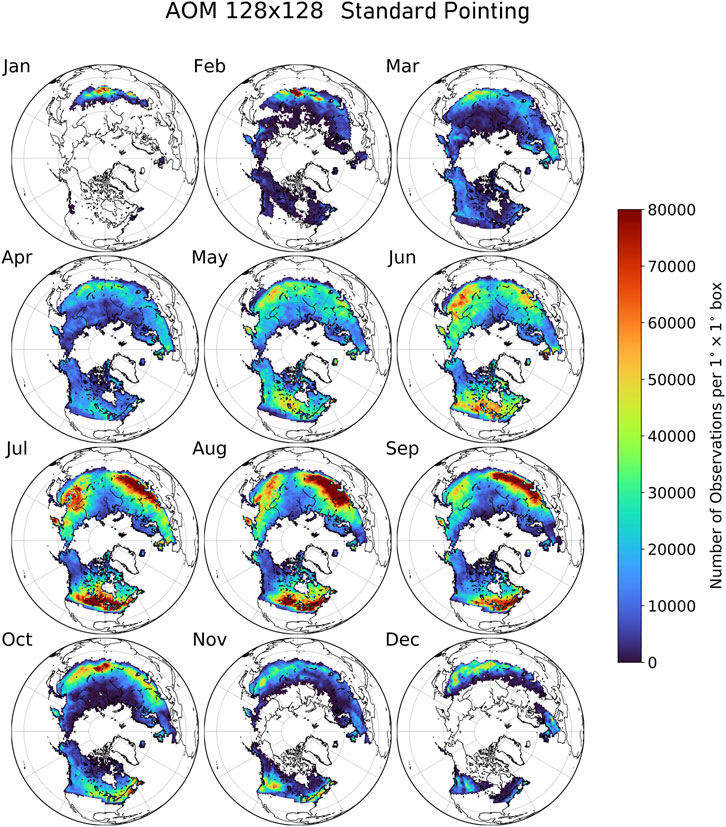
FIGURE 4. Monthly coverage for the 128 × 128 pixel FOV using standard pointing showing the number of observations per 1° × 1°.

FIGURE 5

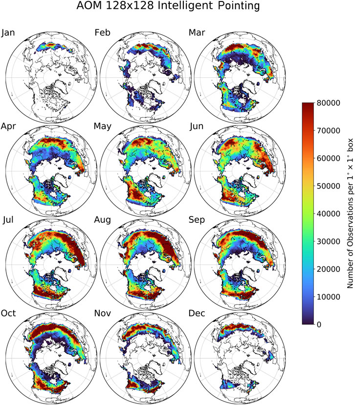
FIGURE 5. Monthly coverage for the 128 × 128 pixel FOV with intelligent pointing showing the number of observations per 1° × 1°.

FIGURE 6

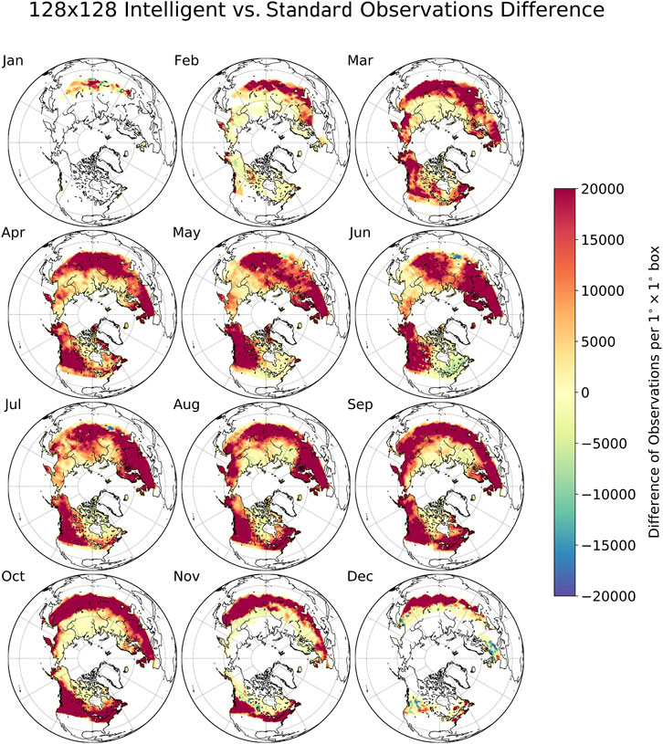
FIGURE 6. Monthly coverage difference (Intelligent–Standard Pointing) for the 128 × 128 pixel FOV showing the difference in the number of observations per 1° × 1°.

FIGURE 7

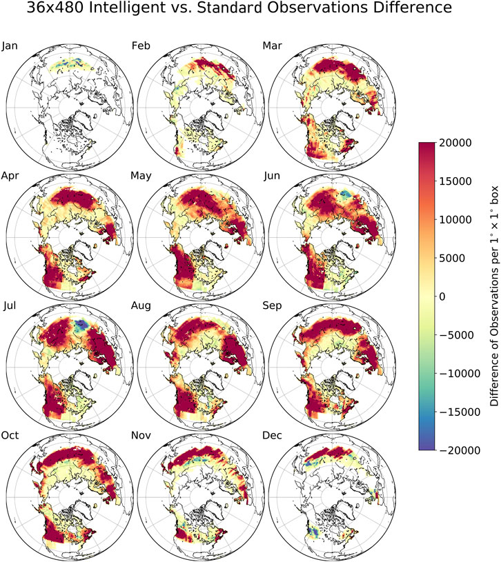
FIGURE 7. Monthly coverage difference (Intelligent–Standard Pointing) for the dispersive spectrometer (36 × 480 pixels/minute) showing the difference in the number of observations per 1° × 1°.

FIGURE 8

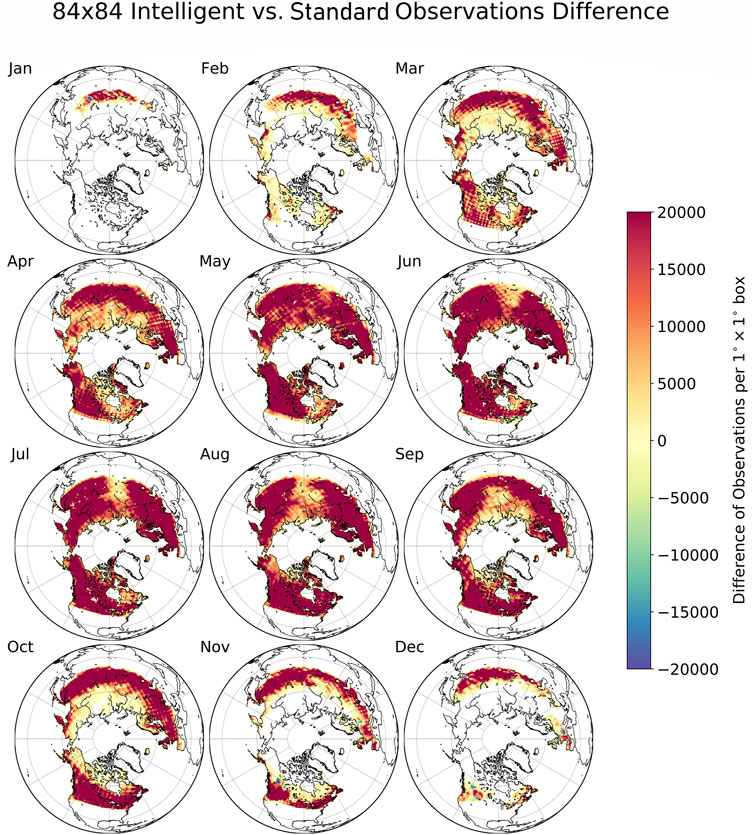
FIGURE 8. Monthly coverage difference (Intelligent–Standard Pointing) for the 84 × 84 pixel FOV showing the difference in the number of observations per 1° × 1°.

FIGURE 9

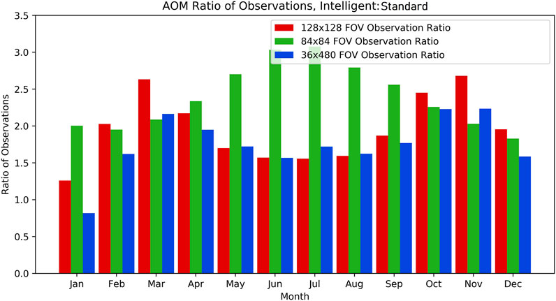
FIGURE 9. Monthly ratio of observations (Intelligent/Standard Pointing) for the three different HEO FOVs.

FIGURE 10

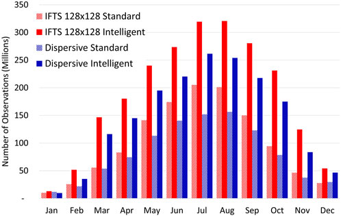
FIGURE 10. Number of cloud-free observations from standard pointing and intelligent pointing for the 128 × 128 pixel IFTS and the dispersive spectrometer.

The monthly difference map for the number of IFTS observations with intelligent pointing minus standard pointing (Figure 6) clearly illustrates the gains that result from intelligent pointing, which reach or even exceed 20,000 additional observations per 1° × 1° grid box over large areas. Very limited areas show a reduction in observations and these could be eliminated if prioritization weighting was relaxed from favoring more northerly regions or low VZA. For the dispersive spectrometer, broad areas reaching ∼20,000 additional observations per 1° × 1° grid box are also observed, but these dense increases are less extensive, while June and July show an area of significant decrease in central Asia. The decreases seem to be centered between the ground tracks near the southernmost part of the area of interest, which can be explained by the low prioritization for southern observations and high VZA observations with intelligent pointing. The 84 × 84 mini-IFTS yielded the largest increases due to intelligent pointing, despite a smaller number of raw observations by more than a factor of two. The monthly ratios in Figure 9 in the winter months, specifically December, January and February are less meaningful since they deal with few observations over a limited area, as shown in the distribution maps. The ratios indicate that intelligent pointing typically yields a factor of 1.5–3.0 more observations than standard pointing since fewer observations are lost due to clouds. The highest ratios (∼3) were observed for the 84 × 84 pixel mini-IFTS during the sunny northern hemisphere summer months of June and July.

4 Discussion and conclusion

In this work, we simulate greenhouse gas observations with standard pointing and intelligent pointing for the current AOM baseline IFTS instrument (128 × 128 pixels), a dispersive spectrometer and a mini-IFTS (84 × 84 pixels), all observing from a three apogee (TAP) highly elliptical orbit (HEO). Even though the IFTS made fewer raw observations than the dispersive spectrometer, it yielded more successful observations in standard or intelligent pointing mode. The increase in observations even with standard pointing results from the better efficiency of the square FOV to scan irregularly-shaped land masses.

However, multiple factors contribute to intelligent pointing efficiency such as the speed of observation and the size and shape or aspect ratio of the Field of View (FOV). A demonstrated advantage is found for a ∼1:1 aspect ratio FOV for cloud avoidance. For the baseline observing parameters under consideration for AOM, the fraction of cloud-free observations is a factor of ∼2 more than in the absence of intelligent pointing. The fraction varies depending on the month due to seasonal variations in the size of the observable area primarily linked to the seasonal cycle of solar illumination for the northern high latitudes, and to a lesser extent, actual seasonal changes in cloud cover. Preliminary simulations suggest that our conclusions for HEO are also entirely applicable to GEO, which is in many ways, an even better vantage point for GHG observations by an IFTS.

Intelligent pointing yields improvements in the number of monthly observations by a factor of about ∼1.5–2.1 for the dispersive spectrometer, ∼1.5–2.5 for the 128 × 128 pixel baseline AOM IFTS and ∼1.5–3.0 for the 84 × 84 mini-IFTS, demonstrating that intelligent pointing is most efficient with a 1:1 aspect ratio and small FOV, followed by a 1:1 and larger FOV, then the dispersive spectrometer with its unbalanced aspect ratio and FOV shape that is poorly-suited for scanning irregularly shaped land masses or observing through the gaps in clouds. Although the small 84 × 84 FOV gave a greater relative increase as a result of intelligent pointing, the most overall observations of any instrument in this comparison were obtained with the AOM 128 × 128 pixel IFTS using intelligent pointing.

These first HEO intelligent pointing simulation results were obtained with fixed pointing grids and without optimization of the priority weights for factors such as cloud, airmass, latitude and history for each instrument configuration. One can envision further efficiency improvements without fixed grids where each individual FOV can be optimally placed in a cloud gap to cover the cloud free areas with a minimum number of FOVS. One can also envision further efficiency improvements via optimization of the priority weights through some iterative process or even application of machine learning algorithms/artificial intelligence, which we intend to explore in future work.

Implementation of intelligent pointing on any satellite mission will require cloud information in the form of cloud masks that correspond to the field of regard (FOR). The focus of this manuscript is on the benefits of intelligent pointing from a data yield perspective, but some comments on implementation are also given here. GOSAT-2 uses a CMOS (complementary metal oxide semi-conductor) video camera with 608 × 1024 pixels that covers an area of ∼30 × 50 km² at ∼0.1 km spatial resolution. The camera has red, green and blue (RGB) detection and 8-bit digitization. An algorithm is applied to utilize output from the 3 color bands of this camera to convert it to a cloud mask in 0.2 s (Suto et al., 2021). For HEO, a key difference is that the satellite is moving much more slowly with respect to the Earth, so sub-second processing to derive a cloud mask like with GOSAT-2 is not required. The early plan for intelligent pointing from AIM-North (Nassar et al., 2019) included a small dedicated 4-kg cloud imager that used a 1280 × 1024 pixel Indium Gallium Arsenide (InGaAs) focal plane array (FPA) covering 0.4–1.7 microns to observe the full Earth disc with a pixel size of ∼10 × 10 km² from 40,000 km altitude. This proposed cloud imagery would be coarser than individual XCO₂ or XCH₄ pixels, since it would only be required to locate the clearest sky regions to point the 512 × 512 km² FOV. AIM-North’s scope was expanded to include meteorological observations from an Advanced Baseline Imager (ABI, https://www.goes-r.gov/spacesegment/abi.html, Schmidt et al., 2017). ABIs fly on the National Oceanic and Atmospheric Administration (NOAA) Geostationary Operational Environmental Satellite (GOES) R, S, and T satellites along with slight variations of the ABI (differing only by one band) on Korean and Japanese GEO satellites. The ABI is a large (∼350-kg) radiometer with 3 FPAs that are used to observe radiance in 16 bands from ∼0.47–13.3 micron and scans the full Earth disk with 0.5–2.0 km pixels every 5–15 min. Details of the method to derive cloud masks from the ABI to be used in pointing decisions for the AOM IFTS remains to be determined. A very simple approach would be to use the radiance in band 2 (0.59–0.69 micron) to make cloud masks, however, this visible band would poorly distinguish between cloud and snow. Adding information from a SWIR band, such as band 4 (1.3705–1.3855 micron) and/or band 5 (1.58–1.64 micron), should enable more robust cloud/snow distinction. Although pixel-by-pixel cloud detection is the most straightforward approach, performance improvements have been reported in the literature when deep learning is used in cloud detection algorithms that find spatial patterns in satellite imagery (Jeppesen et al., 2019).

Another decision with respect to implementation is whether to process the required cloud data from the ABI onboard the satellite (e.g., Thompson et al., 2014; Gorr and Silva, 2021) and provide the pointing commands to the IFTS directly, or whether downlink of the cloud data to the ground, processing to derive the cloud mask and determine pointing locations, followed by uplink of the pointing commands is more practical. For LEO missions with the satellite moving rapidly and the pointing decision required immediately, onboard processing is a necessity for intelligent pointing. For HEO or GEO, the near-real-time downlink of the ABI radiances for meteorology applications will already occur with a latency of minutes (or less) enabling processing the data into cloud masks on the ground. Uplink of the small volume of data for pointing commands could occur with a comparatively relaxed schedule, such as once per hour, like the length of a pointing cycle for simulations in this paper.

As stated in the introduction, current LEO CO₂ and CH₄ satellites only retain a small fraction of their observations (∼7–12%) relative to their raw observations, primarily due to loss of data due to clouds. Intelligent pointing on GOSAT-2 has shown an increase in yield of cloud-free data by a factor or ∼1.8. Our simulations for HEO demonstrate gains ranging from ∼1.5 to 3.0 depending on the size and aspect ratio of the FOV, with room for further improvement related to possibilities for optimization. For GEO, preliminary work suggests that gains will resemble those of HEO since in both cases, the full Earth disk is viewed. This potential for a greater fraction of cloud-free observations from HEO and GEO warrants further consideration of these complementary orbits in the planning of future CO₂ and CH₄ satellite missions and constellation architectures (Crisp et al., 2018). As a subsequent step to simulations like this one, we are also undertaking a more complete Observing System Simulation Experiment (OSSE) to evaluate the ability of such observations to quantify Artic and Boreal CO₂ fluxes from vegetation (forests, tundra) and permafrost thaw in comparison with and in combination with LEO missions.

We have also conducted limited studies on the application of intelligent pointing for air quality observations. Since these simulated observations were made with a dispersive spectrometer with a 545 × 27 FOV aspect ratio, which is significantly different than 1:1 and furthermore since AQ retrievals are typically less sensitive to cloud in the FOV, only modest gains were observed compared with the GHG IFTS. However, our findings demonstrating the advantage of intelligent pointing for GHG observations could have implications for other fields of satellite Earth observation in which clouds are problematic. Ocean color observations (Coakley et al., 2023) or infrared sounding observations in the NOAA Geostationary and Extended Observations (GeoXO) program, are some other areas that could also benefit by studying, developing and implementing an intelligent pointing approach.

Data availability statement

The raw data supporting the conclusion of this article will be made available by the authors, without undue reservation.

Author contributions

RN conceived the study, developed the general methodology and wrote the manuscript. CM ran orbit simulations (GMAT) and developed details of the methodology and initial python code used in the pointing simulations. BK, AF, JI, AG, and SK modified and ran the python code for the pointing simulations. SK and RN generated figures for the publication. CS advised on technical aspects of intelligent pointing implementation and the manuscript presentation. All authors contributed to the article and approved the submitted version.

Funding

This work was funded internally by Environment and Climate Change Canada (ECCC).

Acknowledgments

We thank Dan Sehayek for early exploratory work on intelligent pointing that helped develop the experimental design for this research. We thank Joseph Mendonca for providing feedback on this manuscript. We thank NASA for making MERRA-2 data and GMAT software publicly available.

Conflict of interest

The authors declare that the research was conducted in the absence of any commercial or financial relationships that could be construed as a potential conflict of interest.

Publisher’s note

All claims expressed in this article are solely those of the authors and do not necessarily represent those of their affiliated organizations, or those of the publisher, the editors and the reviewers. Any product that may be evaluated in this article, or claim that may be made by its manufacturer, is not guaranteed or endorsed by the publisher.

References

Bi, Y., Zhang, P., Yang, Z., Wang, Q., Zhang, X., Liu, C., et al. (2022). Fast CO₂ retrieval using a semi-physical statistical model for the high-resolution spectrometer on the fengyun-3D satellite. J. Meteorological Res. 36 (2), 374–386. doi:10.1007/s13351-022-1149-8

CrossRef Full Text | Google Scholar

Burrows, J., Bovensmann, H., Bergametti, G., Flaud, J. M., Orphal, J., Noël, S., et al. (2004). The geostationary tropospheric pollution explorer (GeoTROPE) mission: objectives, requirements and mission concept. Adv. Space Res. 34, 682–687. doi:10.1016/j.asr.2003.08.067

CrossRef Full Text | Google Scholar

Butz, A., Orphal, J., Checa-garcia, R., Friedl-Vallon, F., von Clarmann, T., Bovensmann, H., et al. (2015). Geostationary Emission Explorer for Europe (G3E): mission concept and initial performance assessment. Meas. Tech. 8, 4719–4734. doi:10.5194/amt-8-4719-2015

CrossRef Full Text | Google Scholar

Butz, A., Palmer, P. I., Boesch, H., Bousquet, P., Bovensmann, H., Brunner, D., et al. (2018). ARRHENIUS: a geostationary Carbon process explorer for Africa, Europe and the middle-east, American Geophysical Union, Fall Meeting 2018, abstract #A51R-2515.

Google Scholar

Coakley, M. M., Krimachansky, A., Heidinger, A., Lindsey, D., McCorkel, J., and Sullivan, P. (2023). Cooperative observing strategies for optimizing GeoXO level 1b products. 103rd American Meteorological Society. Annual meeting presentation Available at: https://ams.confex.com/ams/103ANNUAL/meetingapp.cgi/Paper/418807.

Google Scholar

Crisp, D., Meijer, Y., Munro, R., Bowman, K., Chatterjee, A., Baker, D., et al. (2018). A constellation architecture for monitoring Carbon dioxide and methane from space, report from the Committee on Earth Observation Satellites (CEOS) Atmospheric Composition Virtual Constellation greenhouse gas team (October 2018).

Google Scholar

Crisp, D., Pollock, H. R., Rosenberg, R., Chapsky, L., Lee, R. A. M., Oyafuso, F., et al. (2017). The on-orbit performance of the Orbiting Carbon Observatory-2 (OCO-2) instrument and its radiometrically calibrated products. Atmos. Meas. Tech. 10, 59–81. doi:10.5194/amt-10-59-2017

CrossRef Full Text | Google Scholar

Crowell, S., Baker, D., Schuh, A., Basu, S., Jacobson, A. R., Chevallier, F., et al. (2019). The 2015-2016 carbon cycle as seen from OCO-2 and the global in situ network. Atmos. Chem. Phys. 19, 9797–9831. doi:10.5194/acp-19-9797-2019

CrossRef Full Text | Google Scholar

Diner, D., Martonchik, J. V., Kahn, R. A., Pinty, B., Gobron, N., Nelson, D. L., et al. (2005). Using angular and spectral shape similarity constraints to improve MISR aerosol and surface retrievals over land. Remote Sens. Environ. 94 (2), 155–171. doi:10.1016/j.rse.2004.09.009

CrossRef Full Text | Google Scholar

Eldering, A., Taylor, T. E., O’Dell, C. W., and Pavlick, R. (2019). The OCO-3 mission: measurement objectives and expected performance based on 1 year of simulated data. Atmos. Meas. Tech. 12, 2341–2370. doi:10.5194/amt-12-2341-2019

CrossRef Full Text | Google Scholar

Gelaro, R., McCarty, W., Suárez, M. J., Todling, R., Molod, A., Takacs, L., et al. (2017). The modern-era retrospective Analysis for research and applications, version 2 (MERRA-2). J. Clim. 30, 5419–5454. doi:10.1175/JCLI-D-16-0758.1

PubMed Abstract | CrossRef Full Text | Google Scholar

Gorr, B., and Silva, D. (2021). Assessing the value of on-board image processing in observation task planning: the cloud mask problem. AIAA Scitech 2021 Forum. doi:10.2514/6.2021-1468

CrossRef Full Text | Google Scholar

Hill, T., and Nassar, R. (2019). Pixel size and revisit rate requirement for monitoring power plant CO₂ emissions from space. Remote Sens. 11 (13), 1608. doi:10.3390/rs11131608

CrossRef Full Text | Google Scholar

Jeppesen, J. H., Jacobsen, R., Inceoglu, F., and Toftegaard, T. (2019). A cloud detection algorithm for satellite imagery based on deep learning. Remote Sens. Environ. 229, 247–259. doi:10.1016/j.rse.2019.03.039

CrossRef Full Text | Google Scholar

Kasahara, M., Kachi, M., Inaoka, K., Fujii, H., Kubota, T., Shimada, R., et al. (2020). Overview and current status of GOSAT-GW mission and AMSR3 instrument. Proc. SPIE 11530 Sensors, Syst. Next-Generation Satell. XXIV, 1153007. doi:10.1117/12.2573914

CrossRef Full Text | Google Scholar

Krutz, D., Walter, I., Sebastian, I., Paproth, C., Peschel, T., Damm, C., et al. (2022). CO2Image: the design of an imaging spectrometer for CO₂ point source quantification. Proc. SPIE 12233, Infrared Remote Sens. Instrum., 1223306. doi:10.1117/12.2635250

CrossRef Full Text | Google Scholar

Kuze, A., Suto, H., Nakajima, M., and Hamazaki, T. (2009). Thermal and near infrared sensor for carbon observation Fourier-transform spectrometer on the Greenhouse Gases Observing Satellite for greenhouse gases monitoring. Appl. Opt. 48 (35), 6716–6733. doi:10.1364/ao.48.006716

PubMed Abstract | CrossRef Full Text | Google Scholar

McGarragh, G. R., O’Dell, C. W., Crowell, S. M. R., Somkuti, P., Burgh, E. B., and Moore III, B. (2023). The GeoCarb greenhouse gas retrieval algorithm: simulations and sensitivity to sources of uncertainty. Atmos. Meas. Tech. Disc. 2023, 1–52. doi:10.5194/amt-2023-17

CrossRef Full Text | Google Scholar

Molod, A., Takacs, L., Suarez, M., and Bacmeister, J. (2015). Development of the GEOS-5 atmospheric general circulation model: evolution from MERRA to MERRA2. Model Dev. 8, 1339–1356. doi:10.5194/gmd-8-1339-2015

CrossRef Full Text | Google Scholar

Moore, B., Crowell, S. M. R., Rayner, P. J., Kumer, J., O’Dell, C. W., O’Brien, D., et al. (2018). The potential of the geostationary carbon cycle observatory (GeoCarb) to provide multi-scale constraints on the carbon cycle in the Americas. Front. Environ. Sci. 6, 109. doi:10.3389/fenvs.2018.00109

CrossRef Full Text | Google Scholar

Nassar, R., Hill, T. G., McLinden, C. A., Wunch, D., Jones, D. B. A., and Crisp, D. (2017). Quantifying CO₂ emissions from individual power plants from space. Geophys. Res. Lett. 44. doi:10.1002/2017GL074702

CrossRef Full Text | Google Scholar

Nassar, R., McLinden, C., Sioris, C., McElroy, C. T., Mendonca, J., Tamminen, J., et al. (2019). The atmospheric imaging mission for northern regions: AIM-North. Can. J. Remote Sens. 45, 423–442. doi:10.1080/07038992.2019.1643707

CrossRef Full Text | Google Scholar

Nassar, R., Moeini, O., Mastrogiacomo, J.-P., O'Dell, C. W., Nelson, R. R., Kiel, , et al. (2022). Tracking CO₂ emission reductions from space: a case study at Europe's largest fossil fuel power plant. Front. Remote Sens. 3. doi:10.3389/frsen.2022.1028240

CrossRef Full Text | Google Scholar

Nassar, R., Sioris, C. E., Jones, D. B. A., and McConnell, J. C. (2014). Satellite observations of CO₂ from a Highly Elliptical Orbit (HEO) for studies of the Arctic and boreal carbon cycle. J. Geophys. Res. - Atmos. 119, 2654–2673. doi:10.1002/2013JD020337

CrossRef Full Text | Google Scholar

O’Dell, C. W., Connor, B., Bösch, H., O’Brien, D., Frankenberg, C., Castano, R., et al. (2012). The ACOS CO₂ retrieval algorithm – Part 1: description and validation against synthetic observations. Atmos. Meas. Tech. 5 (1), 99–121. doi:10.5194/amt-5-99-2012

CrossRef Full Text | Google Scholar

Pasternak, F., Bernard, P., Georges, L., and Pascal, V. (2016). The MicroCarb instrument. Proc. SPIE 10562, 105621P–1. doi:10.1117/12.2296225

CrossRef Full Text | Google Scholar

Rayner, P. J., Utembe, S. R., and Crowell, S. (2014). Constraining regional greenhouse gas emissions using geostationary concentration measurements: a theoretical study. Atmos. Meas. Tech. 7, 3285–3293. doi:10.5194/amt-7-3285-2014

CrossRef Full Text | Google Scholar

Schaaf, C., and Wang, Z. (2021). MODIS/Terra+Aqua BRDF/albedo daily L3 global - 500m V061. Distributed by NASA EOSDIS land processes. DAAC. doi:10.5067/MODIS/MCD43A3.061

CrossRef Full Text | Google Scholar

Schmidt, T. J., Griffith, P., Gunshor, M. M., Daniels, J. M., Goodman, S. J., and LeBair, W. J. (2017). A closer look at the ABI on the GOES-R series. Bull. Am. Meteorological Soc. (BAMS) 98, 681–698. doi:10.1175/BAMS-D-15-00230.1

CrossRef Full Text | Google Scholar

Sierk, B., Fernandez, V., Bézy, J.-L., Mejer, Y., Durand, Y., Bazalgette, G., et al. (2021). The Copernicus CO2M mission for monitoring anthropogenic carbon dioxide emissions from space. Proc. SPIE 11852, 118523M–118532M. doi:10.1117/12.2599613

CrossRef Full Text | Google Scholar

Staebell, C., Sun, K., Samra, J., Franklin, J., Chan Miller, C., Liu, X., et al. (2021). Spectral calibration of the MethaneAIR instrument. Atmos. Meas. Tech. 14 (5), 3737–3753. doi:10.5194/amt-14-3737-2021

CrossRef Full Text | Google Scholar

Stubenrauch, C. J., Rossow, W. B., Kinne, S., Ackerman, S., Cesana, G., Chepfer, H., et al. (2013). Assessment of global cloud datasets from satellites: project and database initiated by the GEWEX radiation panel. Bull. Am. Meteorological Soc. 94, 1031–1049. doi:10.1175/BAMS-D-12-00117.1

CrossRef Full Text | Google Scholar

Suto, H., Kataoka, F., Kikuchi, N., Knuteson, R. O., Butz, A., Haun, M., et al. (2021). Thermal and near-infrared sensor for carbon observation Fourier transform spectrometer-2 (TANSO-FTS-2) on the Greenhouse gases Observing SATellite-2 (GOSAT-2) during its first year in orbit. Atmos. Meas. Tech. 14, 2013–2039. doi:10.5194/amt-14-2013-2021

CrossRef Full Text | Google Scholar

Taylor, T. E., O’Dell, C. W., Baker, D., Bruegge, C., Chang, A., Chapsky, L., et al. (2023). Evaluating the consistency between OCO-2 and OCO-3 XCO2 estimates derived from the NASA ACOS version 10 retrieval algorithm. Atmos. Meas. Tech. 16, 3173–3209. doi:10.5194/amt-16-3173-2023

CrossRef Full Text | Google Scholar

Taylor, T. E., O’Dell, C. W., Frankenberg, C., Partain, P. T., Cronk, H. Q., Savtchenko, A., et al. (2016). Orbiting Carbon Observatory-2 (OCO-2) cloud screening algorithms: validation against collocated MODIS and CALIOP data. Atmos. Meas. Tech. 9, 973–989. doi:10.5194/amt-9-973-2016

CrossRef Full Text | Google Scholar

Thompson, D. R., Green, R. O., Keymeulen, D., Lundeen, S. K., Mouradi, Y., Nunes, D. C., et al. (2014). Rapid spectral cloud screening onboard aircraft and spacecraft. IEEE Trans. Geoscience Remote Sens. 52 (11), 6779–6792. doi:10.1109/TGRS.2014.2302587

CrossRef Full Text | Google Scholar

Trishchenko, A. P., and Garand, L. (2011). Spatial and temporal sampling of polar regions from two-satellite System on molniya orbit. J. Atmos. Ocean. Technol. 28, 977–992. doi:10.1175/JTECH-D-10-05013.1

CrossRef Full Text | Google Scholar

Trishchenko, A. P., Garand, L., and Trichtchenko, L. D. (2011). Three-apogee 16-h highly elliptical orbit as optimal choice for continuous meteorological imaging of polar regions. J. Atmos. Ocean. Technol. 28, 1407–1422. doi:10.1175/JTECH-D-11-00048.1

CrossRef Full Text | Google Scholar

Veefkind, J. P., Aben, I., McMullan, K., Förster, H., de Vries, J., Otter, G., et al. (2012). TROPOMI on the ESA Sentinel-5 Precursor: a GMES mission for global observations of the atmospheric composition for climate, air quality and ozone layer applications, Remote Sens. Environ., 120 70–83. doi:10.1016/j.rse.2011.09.027

CrossRef Full Text | Google Scholar

Wang, S., Zhang, Y., Hakkarainen, J., Ju, W., Liu, Y., Jiang, F., et al. (2018). Distinguishing anthropogenic CO₂ emissions from different energy intensive industrial sources using OCO-2 observations: a case study in northern China. J. Geophys. Res. Atmos. 123 (17), 9462–9473. doi:10.1029/2018jd029005

CrossRef Full Text | Google Scholar

Wu, D., Lin, J. C., Oda, T., and Kort, E. A. (2020). Space-based quantification of per capita CO₂ emissions from cities. Environ. Res. Lett. 15, 035004. doi:10.1088/1748-9326/ab68eb

CrossRef Full Text | Google Scholar

Xi, X., Natraj, V., Shin, R. L., Luo, M., Zhang, Q., Newman, S., et al. (2015). Simulated retrievals for the remote sensing of CO₂, CH₄, CO and H₂O from geostationary orbit. Atmos. Meas. Tech. 8, 4817–4830. doi:10.5194/amt-8-4817-2015

CrossRef Full Text | Google Scholar

Yang, Z., Zhen, Y., Yin, Z., Lin, C., Bi, Y., Liu, W., et al. (2018). Prelaunch radiometric calibration of the TanSat atmospheric carbon dioxide grating spectrometer. IEEE Trans. Geoscience Remote Sens. 56 (7), 4225–4233. doi:10.1109/TGRS.2018.2829224

CrossRef Full Text | Google Scholar