Improving satellite-based monitoring of the polar regions: Identification of research and capacity gaps

1 Introduction

The Earth’s Polar Regions are experiencing rapid environmental changes with rising temperatures both in the atmosphere and in the oceans (IPCC, 2019). Monitoring these changes, and the resulting effect on the cryosphere of sea ice, glacial ice on land, permafrost, and snow cover, is essential in understanding the drivers of change and the potential consequences those changes may represent for the planet and society. Due to the remote and sometimes harsh environment of the polar regions, satellite remote sensing has been a vital tool in observing and assessing the changes that are taking place. In fact, efforts to provide more comprehensive surveillance and understanding have been increasing since the International Polar Year (IPY) 2007-9. One of the success stories within Europe has been the development of the Copernicus programme of the European Commission; a 5.4 billion € investment for the period 2021–2027, encompassing satellite space and ground systems, and associated data processing services, to provide global Earth Observation and assessment.

In this paper we perform a detailed review of the state of the space-based monitoring with three main objectives:

1) To identify the potential for improving the parameter retrieval from satellite data and for gathering additional satellite variables to monitor the Polar Regions which could have positive impact when assimilating them into modelling/forecast products,

2) To assess the capabilities of future satellite missions (with special focus on the Copernicus Expansion Missions) for polar monitoring, and

3) To study how in-situ field measurements contribute to polar environmental monitoring and improvement of data products.

2 Gaps and limitations of remote sensing for polar monitoring

A comprehensive review of the current status of remotely sensed parameters acquired over Polar Regions is presented and compared with the products provided by the Copernicus service to identify current data gaps. In addition, we perform an assessment of future satellite missions including the Copernicus Sentinel Expansion Missions, planned for launch in the later 2020s, in terms of their benefit for environmental monitoring and the integration and assimilation of their data into forecasting products. We also determine possible synergies between parameters obtained from different satellite missions in order to enhance the information content of specific data products considering the end-users requirements. Finally, we identify the limitations of the currently assimilated variables, as well as the potential of new variables that are relevant for assimilation into models for simulations and forecasts of conditions in the Polar Regions.

2.1 Sea ice parameters

2.1.1 Review and limitation of sea ice concentration and sea ice thickness measurements

Sea ice cover is both an indicator and driver of high-latitude climate change with strong societal and ecological importance. It is a key boundary condition for atmospheric and ocean models, including those used in atmospheric reanalyses, and a benchmark for coupled climate models. Sea ice concentration is a useful variable both for monitoring climate change and for navigation, and helps to determine a number of other important climate variables, such as albedo, the freshwater fluxes between (polar) oceans, and heat transfer between the atmosphere and ocean.

The most prevalent satellite measurements of Sea Ice Concentration (SIC) are carried out using multi-frequency passive microwave radiometers (e.g., AMSR2, SSMIS, and MWRI), typically recording the Earth-leaving radiation at different microwave frequency bands (e.g., C-band: ∼6.9 GHz, Ku: ∼19 GHz, Ka: ∼37 GHz). Measurements at these microwave frequencies do not require solar light, and are not compromised by clouds. They thus offer the all-weather, all-year capability. For a given space-borne passive microwave radiometer, channels with higher microwave frequency (and shorter wavelength) have a better spatial resolution (e.g., the resolution of the AMSR2 89 GHz (W-band) channel is ∼5 km, of the 36.5 GHz channel ∼12 km), albeit with increasing susceptibility to atmospheric effects. Thus, remote sensing of sea-ice concentration from microwave radiometry is always a trade-off between accuracy and spatial resolution (Comiso et al., 1997). An inventory of 30 algorithms for the retrieval of sea ice concentration was compiled in the context of the ESA Climate Change Initiative (CCI) Sea Ice projects (Ivanova et al., 2014). Atmospheric correction (requiring Radiative Transfer Models), weather filtering, correction for land spill-over effects, dynamic tuning of the algorithm tie-points are major elements of a modern passive microwave SIC processing chain, and affect the use of this data in strategic monitoring applications requiring accurate mapping of the sea ice edge or coastal zone, such as navigation and maritime safety.

Tactical monitoring applications are primarily served by data obtained from synthetic aperture radar (SAR) imaging missions (e.g., Sentinel-1, RADARSAT-2,etc.) operating at C-band (∼5.4 GHz). These also provide imaging independent of the polar night and cloud cover. Weather effects such as wind and precipitation over the ocean, however, yield ambiguities in data of SAR systems operated at single-frequency and co-polarization (HH or VV). These issues can be reduced by acquiring data in more polarizations, with modern SAR sensors that are operated with the addition of a cross-polarization channel that provides improved ice versus water discrimination. Another strategy to reduce ambiguities requires the combination of data from two different satellite missions, such as complementing the C-band imagery by data acquired at lower frequencies such as L-band (1.27 GHz on ALOS-2 and SAOCOM satellites). Whilst SAR-based products have substantially higher resolution than those from microwave radiometry, their limitation is that the spatial coverage is restricted to relatively narrow (maximum 500 km) SAR scenes. Therefore pan-Arctic or pan-Antarctic maps require several days of aggregation, or the combination of data from two or more satellites. E.g., the Sentinel-1 mission, presently consisting of two satellites 1-A and 1-B (although recently B has failed), and will be extended by Sentinel-1C. Shortening the time for generating pan-Arctic maps will also be possible with the Radarsat Constellation Mission (RCM) when/if it is seamlessly available to Copernicus users. SAR images are the main input for National Ice Services to produce their ice charts, which are targeted at end-users for navigation. Operational ice charting is at present mostly carried out manually, with trained ice analysts drawing and labeling polygons based on a combination of SAR, optical, and passive microwave data.

Optical spectrometry (e.g., Sentinel-3 OLCI, Sentinel-2, MODIS, and VIIRS) is another tool for monitoring sea-ice concentration with high spatial resolution, but here the main limitation is cloud cover and the need for sunlight.

Interestingly, several investigators have recently adopted multi-sensor approaches to combine the strong points of the individual techniques and reduce ambiguities. For example, SIC products based on a merging of passive microwave and SAR are underway (e.g., Karvonen, 2014). Also, Ludwig et al. (2019) attempted to merge passive microwave with MODIS cloud-free imagery. In all these cases, the rationale for adopting a multi-sensor approach is to build upon the nearly daily complete coverage of the passive microwave products and improve the spatial resolution where SAR or visible imagery is available.

However, with the current observing systems, none of these techniques fully resolve user requirements (both for navigation and ingestion in forecasting models). Moreover, the existing capabilities work best in freezing conditions. When temperatures rise near the melting point and further when surface snow starts melting and melt ponds form at the top of sea ice, the accuracy of most algorithms is greatly reduced (Kern et al., 2020). With increased forecast model resolution, coverage and accuracy, SIC data, in particular from the ice edge and in the coastal zones, are needed. To ensure the delivery of the necessary data at a long-term perspective, fully operational missions with long-term continuity are needed. Multi-sensor techniques with SAR and/or optical must be further explored.

Sea ice thickness is becoming an increasingly important parameter for climate change monitoring due to the observed thinning of the sea ice and the increase of the thin sea ice areal fraction in particular in the Arctic. Sea ice thickness is also very important for operational ice monitoring (ice charting), but until today no large-scale observational capability with the required spatial resolution exists. Estimates of ice thickness in operational ice charts are therefore mostly based on indirect information from ice type classification based on SAR and taking into account meteorological data (freezing degree days).

Radar and lidar altimeters measure the ice freeboard, which is obtained as the difference between the local sea surface and the ice/snow pack surface height. The ice thickness is computed from the ice freeboard using the hydrostatic equilibrium equation making assumptions on ice and snow densities, and on snow depth (Zwally et al., 2008). The discrimination of radar and laser echoes from the ice/snow surface and from the open water surface is based on the surface reflectivity variations (Zwally et al., 2008; Laxon et al., 2013). Some of the satellites carrying this technology are: CryoSat-2, Sentinel-3, and ICESat-2.

One important limitation of altimeter measurements is the lack of precise snow depth measurements, which are fundamental to derive the ice thickness from freeboard measurements. Moreover, the altimetric measurements reveal unacceptable uncertainty when the ice is thin (lower than 1 m). Another limitation is that 1 month of measurements is currently required to obtain a full coverage of the Arctic. The spatial resolution varies depending on the sensor. Radar altimeters such as CryoSat-2 using the SAR technique, as opposed to the conventional pulse-limited approach, employ coherent processing of groups of transmitted pulses to make efficient use of the properties of the signal reflected back from the surface, which provides enhanced spatial resolution and with multilook processing both along-track and across-track. CryoSat-2 therefore has a measurement footprint of 250 m (along-track) and 1.7 km (across-track), compared to 16–20 km of the Envisat RA-2 in both directions. Use of lidar offers further resolution improvement, albeit with the trade-off that the sensor cannot measure through cloud cover. ICESat-2 has a measurement footprint of 13 m. The full resolution of these individual observation points is however only accessible from along-track products, and is smeared in the weekly or monthly mapped products.

Radiometry working at low microwave frequency (1.4 GHz- L-band), such as the Soil Moisture and Ocean Salinity (SMOS) and Soil Moisture Active Passive (SMAP) missions, can retrieve sea ice thickness from brightness temperatures (Kaleschke et al., 2012). However, the ice thickness retrieval with this method is limited to the thickness of less than ∼0.5–1.0 m depending on the salinity of the ice (Kaleschke et al., 2012; Huntemann et al., 2014), since the microwave emission from deeper ice layers is mostly attenuated. The spatial resolution is also limited to ∼25–35 km. Temporal resolution is daily for the sea ice thickness product in the Arctic region. This technique is limited to the freezing period, while radiometric measurements at melting conditions are distorted.

Ricker et al., 2017 produced a merged SMOS and CryoSat data product, covering the entire sea ice thickness range, improving the temporal resolution as well as achieving a significant reduction in the relative uncertainty.

Whether from altimetry or radiometry, the retrieval of sea-ice thickness has reached a relative maturity only for the Arctic, while the Antarctic products are still more experimental.

Operational applications today require high-resolution products over the Arctic with a minimal time delay, which until now is not achieved with radar altimetry nor radiometry. A higher resolution sea ice thickness product (100 s of meters to a few kilometer resolution) is also missing, as well as data during the melt season.

2.1.2 Review and limitation of snow on sea ice

Monitoring the snow-depth on sea-ice is at present the “holy grail” of sea-ice remote sensing. It is an especially important parameter, both for the retrieval of sea-ice thickness from radar altimetry and for ingestion in forecast models (due to the insulation effect of snow and its impact on the surface albedo). Snow-depth on sea ice also has a key role in navigation, as it creates a cushioning and frictional effect that reduces the efficiency of a vessel that is breaking ice.

Several techniques are being investigated for the retrieval of snow-depth on sea ice. Three classes of methods are: 1) from microwave radiometry, especially using low-frequency channels such as those of AMSRs, SMOS, and the future CIMR, 2) from dual-frequency altimetry (e.g., Ka/Ku altimetry combining AltiKa and CryoSAT2, or CRISTAL), and 3) from modelling approaches (snow precipitation from atmospheric reanalysis are advected and accumulated using ice drift information). At this stage, none of these techniques outperforms the others, and all show rather limited accuracy compared to validation data.

There are many caveats for the retrieval of snow-depth on sea ice from satellite data, one of which is the lack of dedicated satellite missions and the relative lack of validation data. However, the planned CRISTAL mission, one of the Copernicus Expansion missions, could be a game-changer in the future (see Section 3.2 for more information).

2.1.3 Review and limitation for ice drift and ice deformation

The use of satellite image pairs for ice drift retrieval has been investigated in several studies (Lavergne et al., 2010; Hollands and Dierking, 2011; Demchev et al., 2017; Korosov and Rampal, 2017). Two approaches are popular: 1) correlation techniques and 2) tracking of distinct features. In the former approach, small windows are distributed as regular grids in the master image. For each window its shift of position in the second image is systematically determined by applying spatial correlation (“pattern matching”). The search can be organized in resolution pyramids and cascades. Feature tracking works by identifying distinct ice cover structures such as distinct floes, ridges, leads, or cracks in the primary image and trying to find them in the secondary image. Image data originating from optical, SAR, scatterometer or passive microwave sensors are used. Drift vectors obtained from pattern matching are mostly shown on the vertices of a fixed regular grid (Eulerian approach). If single distinct features are tracked, the grid resulting from connecting single adjacent drift vectors is irregular. Pattern matching and feature tracking can be combined. Rotational motion of ice floes requires additional retrieval procedures. The advantage of using satellite images compared to data from drifting buoys is the much higher high spatial density of drift vectors. When using different imaging systems (SAR and radiometers) the spatial resolution and areal coverage of the retrieved drift fields vary. Historically sea-ice drift vectors from SAR and optical imagery were retrieved from individual orbit data, while daily averaged imagery were used for passive microwave and scatterometer data. Lavergne et al. (2021) recently demonstrated the feasibility of retrieving sea-ice drift from individual orbit data of the AMSR2 mission, in preparation for CIMR.

When sea-ice drift estimates are available from different sensors, they can be merged for generating a multi-sensor drift product. The multi-sensor product aims at gaining confidence in the retrieved ice motion by a synergetic use of several instruments and reducing the number of missing data. Current merging methodologies are rather crude and limited in scope (see known limitations and gaps below).

The instantaneous (sub-second) sea ice motion along the line-of-sight (LoS) between the radar and a surface element can be retrieved from the Doppler frequency derived from SLC (single-look complex) data based on a single SAR scene (Kræmer et al., 2018). Instantaneous LoS components of drifting ice can also be derived from along-track interferometry, but in this case, again two images are required from a satellite tandem (two identical SAR instruments) for which the along-track (temporal) baseline is on the order of milliseconds and the across-track baseline is short enough to minimize the influence of ice topography on the interferometric phase (Dammann et al., 2019). The spatial resolution is higher than for the Doppler approach. For operational applications and direct comparisons with model simulations, these two approaches are of limited value because they only provide a single vector component of the ice motion taking place within an extremely short time interval.

The calculation of deformation parameters (divergence/convergence, vorticity, shear, and total deformation) is carried out based on the retrieval of displacements, e.g., (Weiss, 2013). Such data can be obtained from arrays of buoys (Itkin et al., 2017) or pairs of satellite images (Lindsay and Stern, 2003), with the restrictions regarding spatial density or temporal resolution as discussed above. Hence, uncertainties in the displacement vectors affect the estimates of deformation parameters. The latter is calculated from line integrals that are calculated on the boundary of grid cells (in the case of satellite images) or of buoy arrays (Dierking et al., 2020). Features resulting from deformation events (ridges, leads, etc.) can also be identified in SAR images. The detection performance depends in particular on spatial resolution and on frequency—L-band is better suited than C- or X-band (Dierking and Dall, 2007; Dierking and Dall, 2008). Providing that the time gaps between image acquisitions over a given area are sufficiently small (depending on the mobility of the ice cover), L-band data are regarded as useful for ice drift retrieval. For employing L-band satellite data in operational ice charting, requirements have to be met such as latency for the availability of needed data products, coverage of regions of interest, and long-term continuity of data acquisitions. This is being considered in the planning of ESA’s ROSE-L mission. For the classification of ice structures such as deformation zones and different ice types, L-C-band tandem satellite missions are favored by the ice services.

2.1.4 Review and limitation for ice type and ice edge

The measurement of ice type and ice edge for the ice chart production in operational services is mostly carried out using SAR images at wide-swath modes. With scatterometer and passive microwave radiometer the entire Arctic and Antarctic can be covered within a short time and long-term temporal variations of regional ice type distributions can be monitored, although at the cost of much lower spatial resolution and reduced accuracy at the ice edge and in the coastal zone. While the fine resolution of pixels in SAR images mean that they cover only one ice type, the much larger pixel size of scatterometer and PMW radiometer images means that they may often contain mixtures of different types. These are therefore not well suited for operational ice mapping. Besides, for the manual generation of ice charts mentioned above, there is an increased interest in applying automated procedures, considering the growing number of available satellite images and the potential arising from merging data of different sensor types, as is demonstrated in several published studies (see, Dierking, 2021, for an overview). The separability of ice types in microwave data depends on frequency, polarization, incidence angle, and the spatial resolution. The interpretation and analysis of the images rely on the intensity and textural variations which are caused by differences in surface roughness, volume inhomogeneities (both on length scales of the wavelength), and macro-scale ice structures (e.g., ice ridges, leads, and floe margins), all of which can vary considerably with the time of year and prevailing environmental conditions.

2.1.5 Review and limitations of iceberg detection

Icebergs represent a serious risk for ship navigation and offshore structures. The detection of icebergs, both manually and automatically, requires high spatial resolution satellite products as most icebergs are less than 200 m in size. This is only available with SAR or optical sensors, the latter being of limited or no value in case of cloud coverage and darkness. To cover wide regions within short time intervals, a wide-swath mode SAR product is preferred by the operational ice centers which limits the achievable spatial resolution. Hence, iceberg monitoring will benefit from satellite constellations which provide the necessary coverage with two or more satellites and on the other hand allow the selection of imaging modes with higher spatial resolution. At present, different automated detection algorithms are designed and tested both for Arctic and Antarctic conditions, based on CFAR (Constant False Alarm Rate) approaches, object detection, or segmentation, and considering also multi-frequency and/or multi-polarization SAR image acquisitions (Dierking, 2021). Preliminary results of recent investigations reveal that L-band SAR may have some advantages for iceberg monitoring, particularly with the detection of icebergs embedded within sea ice. Icebergs in the Antarctic have also been monitored using microwave radiometers (e.g., Silva et al., 2006), but have to be very large, of the order of 10 nautical miles across.

2.1.6 Review and limitations of ice and ocean surface temperature

The Ice Surface Temperature (IST) is one of the most important components in the Arctic and Antarctic surface-atmosphere energy balance. The surface temperature strongly affects the atmospheric boundary layer structure, the turbulent heat exchange, and sea ice temperature controls sea ice melting and growth rates. Advanced thermodynamic sea ice models treat the temperature of the snow and ice surfaces as key parameters for freezing and melting of sea ice.

Measurements of the Sea Surface Temperature (SST) and Ice Surface Temperature (IST) using satellite infrared radiometry is a challenge because of difficulties in distinguishing clouds from snow-covered surfaces, as both appear white in the visible and cold at thermal infrared wavelengths. The SLSTR (Sea and Land Surface Temperature Radiometer) instrument onboard Sentinel-3 provides sea, ice and land surface temperatures. The accuracy of the global sea-surface temperature maps is better than 0.3°C, with a spatial resolution of 0.5 km. This accuracy is sufficient for using this data in model assimilation and validation schemes, if there is a quantitative description of the uncertainty provided.

Deriving the temperature profile through the snow and ice layers, from the surface down to 0.5 m into the ice, is feasible from a combination of the available satellite data. The satellite data used for that are thermal infrared (TIR) and microwave radiometric data at different wavelengths and polarizations from 1.4 GHz (SMOS and SMAP) to 89 GHz (AMSR). The satellite channels of lower frequencies can retrieve temperatures from deeper levels in the snow and ice. The future CIMR mission will provide IST and SST with better accuracy and resolution than the AMSR products.

The satellite sensors are sensitive to changes in snow emissivity, associated primarily with snow precipitation and snow cover metamorphosis processes and with melting processes initiated by surface air temperatures around the freezing point of water. This is primarily affecting the simulated temperature estimates in the snowpack.

2.2 Land parameters

2.2.1 Review and limitations on snow on land measurements

Snow cover is highly sensitive to changes in temperature (freezing/thaw) and precipitation (snowfall, rain, hail) and directly affects the albedo and thus the energy balance of the Earth’s surface. It is a relevant input parameter for weather forecasts and climate change observations. Snow stores a significant mass of water and, with its high dynamic, has a strong effect on regional and global energy and water cycles.

The main technology used for snow cover fraction estimation is medium resolution spectrometers such as Aqua/Terra MODIS, Envisat MERIS/AATSR, AVHRR and in the last years VIIRS and Sentinel-3. More or less consistent climate records can then be established from 1980 - today. Most of the techniques are based on utilizing the Normalized Difference Snow Index (NDSI) (Salomonson and Appel, 2004) which ranges between 0% and 100%. The typical resolutions based on these instruments are 250–1,000 m. Due to the use of optical sensors, polar night and clouds are a clear limitation of the measurements. Therefore the services do not start producing data before March and end in October. In particular, the estimates of the first snowfall in the autumn is uncertain due to a combination of cloudy conditions and if the first snowfalls are late, the services might have stopped providing data. Other challenges for this type of data are: 1) Sub-pixel scaled patch snow cover which can reduce the data accuracy. 2) Dense forests often completely absorb the signatures from snow on the ground. 3) Steep mountainous terrain leads to shadows at north slopes, which produce incorrect estimates of the snow cover fraction if the terrain is not properly corrected for. These can partly be addressed using higher resolution sensors such as Sentinel-2.

Existing snow cover services (CCI Snow, Copernicus Snow) focus all on latitudes below the Arctic Circle where light conditions and favourable cloud cover allows for consistent products and services using medium resolution optical radiometers (MODIS/Sentinel-3). In order to monitor Arctic environments considerable efforts need to be done to take into account results from alternative sensors (passive and active microwaves), and perhaps also use signals in the infrared end of the spectrum from radiometers. A complete and consistent Arctic snow cover product will probably involve using many of the available types of data, in addition to multi-temporal interpolation techniques.

Until recently, it has not been possible to measure snow depth using satellite data. Recent results in Lievens et al. (2019) suggest that the co-/cross-polarization ratio in radar backscatter at C-band SAR from Sentinel-1 has some sensitivity towards snow depth. This approach should be studied further for Arctic regions.

Snow water equivalent (SWE) is an ECV (Essential Climate Variables) and is defined by the density multiplied by the depth of the snow and indicates the amount of liquid water that a snow-mass in a unit area (1 m²) will translate into. SWE can be measured using passive microwave (PMW) radiometer instruments such as SSM/I and AMSR-E, and CIMR will complement these measurements. PMW techniques to measure SWE utilize the fact that radio waves at different frequencies have different extinction coefficients (damping) by the snow. The main limitation of accurate measurements is that PMW techniques are unable to measure SWE in mountains due to the coarse resolution. Possible solutions to this lie in either using radar backscatter changes using high-frequency SAR (X and Ku-band) (Rott et al., 2010) or using the change in the interferometric phase (Guneriussen et al., 2001). The ROSE-L mission utilizing the improved coherency could bring interferometric SWE retrieval a step further. In several projects (e.g., GlobSnow and CCI Snow) the Finnish Meteorological office (Pulliainen, 2006) together with collaborators have developed a global service that utilizes PMW together with data from the meteorological weather station network to provide global estimates of SWE (http://www.globsnow.info/).

Snow melt can be monitored with passive microwave (PMW) radiometers but with a coarse (25 km) resolution. Higher resolution sensors such as scatterometers can also be used (5 km), but in mountainous terrain C-band SAR seems to be the best option (50–100 m, weekly temporal resolution). The main technique for measuring the presence of wet snow is by change detection against a dry snow reference or preferably an average over as many dry snow scenes as possible. Nagler and Rott (2000) suggested this method for ERS-1.

The technology used for snow avalanche detection depends on the spatiotemporal scale of a monitoring or detection purpose. For regional avalanche forecasting, daily knowledge of spatiotemporal avalanche activity is critical. The main technology used for such a monitoring task is high resolution, radar SAR satellite data. Studies have shown the potential of C-band Radarsat-2 data and in recent years, C-band Sentinel-1 data (e.g., Eckerstorfer et al., 2017). This technique has been demonstrated in Northern Norway and for specific Arctic regions, and should be applicable for mountain areas too. Snow avalanche monitoring can be an important input to snow avalanche services, and improve the accuracy of avalanche warning services.

2.2.2 Review and limitations on permafrost

Knowledge of permafrost distribution and dynamics is relevant both for operational activities (transport, construction), for understanding potential health hazards from pathogens released from thawing permafrost, and for understanding its interactions with ecosystems and climate change. The main permafrost variables are (Bartsch et al., 2014).

• Ground temperature profile [K] (required parameter by Global Climate Observing System (GCOS) for the Permafrost ECV)

• Active layer thickness [m] (required parameter by GCOS for the Permafrost ECV)

• Permafrost extent/fraction (additional ECV parameter)

Those cannot be directly observed from space. However, in some cases, they can be estimated based on proxies (land cover, ground deformation, water storage, and lake extent) or determined from a combination of modeling and satellite data products of ground temperature, soil moisture, vegetation cover, and snow cover. While the proxy approach is generally rather limited in scope (Trofaier et al., 2017), it was shown that a combination of ensemble runs of a transient permafrost model driven by a time series of satellite-derived land surface temperature is the optimal method to characterize the three permafrost variables (Bartsch et al., 2021).

More advanced development is needed to have a good assessment of permafrost. Only sparse in situ evaluations of the permafrost fraction are available (for example, ground temperature from boreholes in the GTN-P network or active layer thickness at CALM sites), strongly complicating validation for this parameter. The quality of the active layer thickness predictions depends strongly on the quality of the prescribed ground stratigraphy.

Currently, there is no consistent and frequently updated global map of the parameters permafrost temperature and active layer thickness, as required by GCOS (GCOS-200) based on Earth Observation (EO) records, so that permafrost change detection is only possible at localized sites with in situ observations. ESA’s Permafrost CCI project aims at providing such information for different epochs for the first time, and has released a provisional dataset with annual files for the Northern Hemisphere (north of 30°) for the period 1997–2019, based on results from the transient permafrost model CryoGrid constrained by satellite data (Obu et al., 9999). The products from the ESA Permafrost CCI project should be uptaken by Copernicus. Additional estimates of the permafrost extent could be provided in some cases based on the detection of land surface movements and snow structure changes in regions underlain by permafrost. Permafrost degradation can locally lead to rapid elevation changes in the order of several meters, and high spatial resolution and regular repeat observations for permafrost regions are required to observe ground motion due to changes in the state of permafrost. In addition, the location and extent of permafrost is difficult to assess since much of the permafrost in the Northern Hemisphere is covered by boreal forest. ROSE-L, CRISTAL, and CIMR will offer improved capabilities for permafrost monitoring. Higher coherence and improved capacity to penetrate vegetation of L-Band versus C-band are advantages of L-Band SAR with respect to C-band Sentinel-1 for deriving subsidence and motion (ESA, 2019). Low frequency SAR also has a better sensitivity to freezing state and wetness of soil. In addition, CRISTAL’s Ku-Band will allow deriving melting conditions of snow and snow structure changes, which are relevant for ground thermal properties, and can be used to estimate ground temperature and permafrost extent (Kroisleitner et al., 2018).

The European Ground Motion service has been implemented as a new Copernicus Service Element within the Copernicus Land Monitoring Service to provide information regarding natural and anthropogenic ground motion over the Copernicus Participating States. Scenes with periglacial landscapes, i.e., regions with significant freeze/thaw cycle, and scenes with seasonal snow cover are challenging for Sentinel-1 InSAR and are currently excluded from the service (EEA, 2020). The improved capabilities of CRISTAL, and ROSE-L are expected to address these shortcomings, and the Ground Motion Service should then be extended to cover the circumpolar Arctic area.

2.3 Ocean parameters

2.3.1 Review and limitations for water biogeochemistry

The climate-driven changes within the atmosphere, cryosphere and ocean have wide-ranging consequences for Arctic marine ecological dynamics. Ocean colour remote sensing is the only established satellite technique that opens a window onto ocean biology, especially via the quantification of primary producers: Marine phytoplankton, the base of the marine foodweb and responsible for more than 50% of the produced organic carbon on Earth, is detected via its major pigment, chlorophyll-a (Chl). Ocean colour is the change in the colour of the ocean, and other water bodies such as seas and lakes, due to the substances dissolved and particles suspended within the water. Primarily this remote sensing technique derives the spectrum of marine or other surface water reflectance (also defined as remote sensing reflectance, RRS) from satellite observations. In turn, RRS is used to derive products of inherent optical properties (absorption and backscattering coefficients, marine fluorescence) and concentrations of optically significant constituents present in the upper layer of the ocean (e.g., Chl, suspended sediments (SPM) and coloured dissolved organic matter (CDOM), and since 2020 also phytoplankton functional types (PFT)) from multispectral sensors using the information of several wavebands from 400 to 1,080 nm. In addition to the RRS products at each waveband, also the daily average photosynthetically available radiation (PAR) at the ocean surface is available.

Nearly all ocean color sensors (e.g., SeaWiFS, MODIS, MERIS, and OLCI) are low earth polar-orbiting satellites flying in a sun-synchronous orbit, therefore acquiring also polar observations. If sunlight, sea ice and weather conditions allow, valid data from several orbits per day can be obtained. The only geostationary ocean color missions so far, GOCI and GOCI-II, are not obtaining satellite information in polar areas (Ryu et al., 2012). Data has been recorded first by the ocean color sensor Coastal Zone Color Scanner (CZCS) from 1978–1986, since 1996 data is recorded continuously by many different sensors and the sensors’ capabilities have improved since then. Currently, the spatial resolution of RRS products ranges from 300 m (OLCI on Sentinel-3) to 1 km (MODIS) for globally acquiring ocean colour sensors. The merged SeaWiFS-MODIS-MERIS-VIIRS-OLCI (from 1997 until today) data sets from Copernicus Marine Environment Monitoring Service (CMEMS, https://marine.copernicus.eu/) and Ocean Color Climate Change Initiative (OC-CCI, https://www.oceancolour.org) provide 4 km resolution globally. Since May 2021 from CMEMS OLCI data at 300 m scale for the entire sea and even higher resolution (100 m × 100 m) data on turbidity, Chl and SPM for the coastal waters within 20 km off the shoreline based on Sentinel-2 MSI data are available for the Arctic and European regions waters.

Since Chl and RRS (or normalized water-leaving radiance) are ECVs for climate purposes, GCOS specifies the uncertainty requirements with 30% for Chl and 5% for RRS at blue and green wavelengths, and a stability per decade of 3% and 0.5%, respectively (Sathyendranath et al., 2019).

Based on user consultation results, the uncertainty information is delivered together with the parameter-related product in the in most OC-CCI and CMEMS ocean color products, while operational level-2 products from the satellite sensor agencies (NASA, ESA, EUMETSAT, etc.) do not provide uncertainties considering accuracy based on validation with in-situ and error propagation within the applied algorithm.

Although CMEMS provides ocean colour products at 300 m from OLCI/S-3 and for the Arctic coast at 100 m scale from MSI/S-2, observation of colour in inland waters is not adequately supported, since missions providing such data are focused on land applications (e.g., Sentinel 2 or Landsat 8). Such missions have limited capabilities for retrieval of SPM (turbidity) and Chl, but their sensors’ signal to noise ratio is too low to meet the requirements to obtain valid data over dark waters (see mission requirements presented in IOCCG (International Ocean Colour Coordinating Group) 2018) and especially products on CDOM and PFT are missing at high resolution. Assuming that issues of calibration are addressed, improvements to the capability of Sentinel 2 or Landsat 8 sensors, but also to the new arising high spatial and high spectral resolution sensors, such as PRISMA and EnMAP, could partly meet these requirements, along with High Altitude Pseudo-Satellites (or High Altitude Platforms: HAP, which are aircrafts flying ∼20 km high in the stratosphere) or nanosatellites (Groom et al., 2019). Still no products to characterize spectrally the underwater light are missing, especially regarding the attenuation of UV light. Algorithms exist, but are only applied non-operationally (e.g., Oelker et al., 2022).

For time series analysis of the properties, often the temporal resolution is too low, which is especially the case in the polar regions. For more than half a year no satellite observations are possible because of no or too little incident sunlight, even during sun-light conditions weather conditions are very often dominated by very high waves, sea ice coverage and cloud coverage making detection of ocean color impossible or via adjacency effects deteriorating retrievals. Merging of the same ocean color products from different sensors can improve tremendously the coverage (see Losa et al., 2017). However, when there is very low or no sunlight, coupled biogeochemical-ocean circulation-ice models well-calibrated (also by data assimilation) with remote sensing products and quality controlled in situ data must fill the gap.

Information on chlorophyll fluorescence is only available as product from MODIS as fluorescence line height (FLH); still, this product is difficult to be directly used as indicator of phytoplankton health and other physiological features (nutrient limitation, etc.), and requires dedicated interpretation. In general, retrievals on chlorophyll fluorescence are questionable in polar oceans: the spectral range of RRS data used in their retrieval is here at the noise level due to the low Sun in this region.

Although in situ validation and other forms to ensure the assessment of OC product stability is mostly well-coordinated, it needs to continue and be sustained. Round-robins to develop Fiducial Reference Measurements (FRM) with clear uncertainty and protocol are still sparse and need to be enlarged (e.g., Tilstone et al., 2020). Especially in the polar oceans sampling is sparse, due to difficult access of the region and the exploitation of using autonomous platforms’ optical data needs to be further developed and harmonized, as it is well on the way for the bioARGO floats.

Especially the Supervised Vicarious Calibration (SVC) platforms need to be sustained. In 2018 the SVC Marine Optical BuoY (MOBY) was not able to take measurements for most of the year and also Boussole was on and off, so only the coastal FRMs from AERONET-OC (https://aeronet.gsfc.nasa.gov/new_web/ocean_color.html) could provide SVC. This limited especially the ability to characterize S3B OLCI OC products and delayed its L2 products to become operational only in March 2019. Therefore SVC needs to be sustained and enlarged by at least two more platforms to secure VC of sensors.

2.3.2 Review and limitations of sea surface salinity, temperature, sea surface height, and currents

Sea Surface Salinity (SSS) is a key indicator of the freshwater fluxes and an important variable to understand the changes the Arctic is facing. Since in situ salinity measurements are very sparse in this region, remote sensing salinity measurements are of special relevance.

The salinity of the ocean is measured using L-band passive microwave radiometers. The three L-band missions—the SMOS mission (the first on launched in 2009); the NASA Aquarius mission; and the NASA SMAP (Soil Moisture Active Passive) observatory provide an unprecedented source of salinity information over the Arctic Ocean, which can be assimilated in the models and therefore improve the outputs of the model. The products are served by different institutions, with an spatial resolution of 25 km, and daily served averaging 9 days of data to improve accuracy (Martínez et al., 2022).

The retrieval of sea surface salinity in cold oceans is a challenge, since the sensitivity of the brightness temperatures to sea surface salinity gets considerably reduced when the sea surface temperature is below 10°C. Moreover, some undesired effects are present in the brightness temperatures acquired by the radiometers, such as the land-sea and ice–sea contaminations, which affect the quality of the salinity retrieval close to coasts and ice edges.

A known limitation is that measurements near the coast (less than 50 km) will suffer from land-sea contamination errors, and also on sea-ice contamination. The product could be improved if the combination of different sensors (i.e., SMOS and SMAP) is assessed. There is an urgent need for in situ measurements of salinity in the polar regions. A sufficient in situ database would not only provide a robust assessment of satellite SSS uncertainties in the Arctic Ocean, but also support the retrieval algorithm refinement, leading to enhanced satellite salinity products.

CIMR will record brightness temperature at L-band, and will thus continue the SSS capability of SMAP and SMOS. The spatial resolution of CIMR will not necessarily be better than that of current missions, but the better radiometric resolution of the L-band channel, and the availability of collocated SST and wind retrievals (from higher microwave frequencies) will result in more accurate SSS retrievals, even in cold polar waters (Kilic et al., 2021).

The Sea surface temperature measurements are similar to the ice surface temperature but on ice free regions, so please refer to the ice surface temperature chapter for more information. One of the primary objectives of CIMR is to provide accurate SST with ∼15 km spatial resolution, mainly from the C-band channels.

Satellite measurements of Sea Surface Height (SSH) are based on the data provided by Radar altimeters. Such instruments measure the range between sea surface and instrument antenna. Then, Sea Surface Height can be estimated, if satellite height is known. The resulting measurements, once corrected from atmospheric contributions, contain two main contributions: the oceanographic signal due to currents, tides, heat content and atmospheric load; and the undulations of the geoid. The oceanographic signal, away from the strongest currents, is of the order of 20 cm and varies in time. The undulation of the geoid, on the contrary, is much bigger and constant at typical oceanic scales. If the geoid is not sufficiently well known, which has been the case for most of the time, temporal anomalies have to be computed (Sea Level Anomalies) and the mean sea level due to ocean currents (Mean Dynamic Topography) has to be independently estimated and added (Robinson, 2004).

From a technological point of view, Radar Altimeters can measure Sea Surface Height at their nadir with a footprint of the order of 7 km (Robinson, 2004). During the last years a new generation of radars that use the Synthetic Aperture approach have been developed (e.g., Sentinel-3 constellation; e.g., Ray et al., 2015). In spite of the improvements in the instrument, all current altimetric measurements are flawed by the same problem: the sampling limitations due to their swath. To solve this limitation a new mission concept, the SWOT mission, launched in December 2022, is expected to be able to provide high resolution maps of sea level in the years to come. The future Copernicus Sentinel Expansion Mission CRISTAL mission will allow computing the Mean Dynamic Topography inside the Arctic Ocean, even in the presence of sea ice.

A specific limitation of ocean sea level measurements in the Arctic is the presence of sea ice, although adequate retrackers within leads can be exploited to provide at least monthly averaged sea level maps (Armitage et al., 2016; Prandi et al., 2021).

Measuring ocean currents from satellites is a key challenge of satellite oceanography. The basic principle of the direct measurement of velocities relies on the Doppler effect, i.e., on the change of frequency of the returned signal. Such measurements are currently done by Synthetic Aperture Radars (SAR), allowing for the retrieval of surface velocities (see Ardhuin et al., 2018 for a short review). At present, velocities can be estimated from indirect measurements such as: Sea Surface Height, Sea Surface Temperature, Sea Surface Salinity, a sequence of tracer images or Surface Winds. However, the only truly operational approach to the retrieval of ocean velocities is based on applying the geostrophic approximation to Sea Surface Heights (SSH) measurements provided by altimeters and, eventually, complementing these measurements with wind measurements.

3 Discussion and recommendations

3.1 Better use of in situ measurements, including- citizen science

The rapid pace and highly dynamic interactions of the changing Arctic into a new regime, unrestricted and timely access to scientific observations are crucial for monitoring a sustainable and prosperous Arctic. Unrestricted and timely access to in situ scientific observations and model forecasts underpins evidence-based decision making. Information from Copernicus can be useful in supporting operational monitoring activities such as production of ice charts, maritime navigation, weather forecasting, environmental impact analyses, emergency response, and others. These products are also regularly utilised by researchers whose needs vary considerably depending on the science they are delivering. The commonality linking the needs of both the operational and the research communities is the need for accurate products, with known uncertainties. Thus, an ongoing campaign of validation and calibration (Cal/Val) throughout a product’s lifetime is mandatory. Though, performing Arctic scientific research can be difficult, expensive, and time-consuming to rely on measurements solely from field sites. As a result, in situ measurements in the Arctic are spatially and temporally sparse.

The Copernicus programme is organised in three components, 1) a space component, 2) an in situ component and 3) a service component. The in situ component is aimed at ensuring coordinated access to observations from airborne, seaborne, and ground-based installations. As a result, in situ observations must play an important part within the Copernicus Services. The analysis of the QUIDs (QUality Information Documents) for some of Copernicus’ polar products revealed that the lack of temporal and spatial in situ data in the polar regions is problematic in assessing the quality of these products, as well as severely compromising calibration and validation activities. The results clearly present that validation and quality control of many, if not all, Copernicus products within the Polar Regions is at best poor. Some products in Copernicus Thematic Assembly Centers (TAC) shows major shortfalls, which include: 1) significant lack of in situ observations, possibly combined with the lack of knowledge of where to access some datasets (reference), meant that the protocols laid out in the Cal/Val guidelines cannot be performed. 2) Evaluations that are performed in the Polar Regions do not run over an annual cycle, or in different Polar Regions, and therefore resultant products may not be representative, 3) a general acceptance that the quality of a polar product may be inferior to mid-latitude regions, but with no mechanism to investigate possible solutions, and 4) instances where no validation is performed in the Polar Regions. Therefore, the accuracy of products in these regions cannot be assessed. This suggests some products for the Polar Regions may be inferior due to calibration and validation being performed at lower latitudes, or over limited spatial or temporal periods. Once the QUIDs have been produced we could find little evidence of incentives for developers to improve products, or to provide solutions to known inadequacies. This could be attributed to poor dialogue between the broader European polar research and monitoring community and the Copernicus Services (and associated TACs).

The evidence gathered in KEPLER suggested that citizen science and the European polar research community are presently underutilised by the Copernicus’ Services. During the process of addressing these aims, results revealed a lack of 1) dialogue between Copernicus Services and citizen science (CS) projects; and 2) engagement by the Copernicus Services with the major European Polar bodies and EUfunded programmes (e.g., EU-PolarNet and the Horizon 2020 -EU Polar Cluster projects). Approximately four million people live in the Arctic with significantly increasing visitors to this area. Taking advantage of this exceptional knowledge-base, through the co-production of knowledge via CS, without compromising scientific rigor, is a great opportunity to help advance both scientific knowledge and engagement. Empirical studies of field-based CS programmes have shown that participation in CS increases scientific literacy, the promotion of knowledge, and the understanding of scientific concepts and processes (Aristeidou and Herodotou, 2020). Additionally, CS brings noteworthy contributions to projects where the research can benefit from their many unique perspectives, skill sets, and knowledge as well as identifying a research topic or disseminating results (Lewandowski et al., 2017). Surveys have shown that people were more confident in hypothetical CS findings when professional scientists were involved to some degree, compared to situations in which only citizen scientists were involved (Lewandowski et al., 2017). This reinforces the need for co-production and co-design of CS projects between scientists and the public. Themes from Shirk et al., 2012 suggest that “Co-Created projects” seem to best embody the goals and expectations of both scientists and the public through co-production and co-development of a CS programme. The visibility of the Copernicus Services to the average European citizen would increase incredibly if their products were regularly utilised within CS projects. Moreover, envisage the benefit to science if the power of CS could be applied to the validation and/or calibration of the Arctic products delivered by Copernicus Services or ESA.

As one of the biggest distributors of environmental products and services in Europe the Copernicus Services should play a proactive role in 1) making sure their products are usable by CS projects, 2) ensuring CS projects can enhance the accuracy and usability of their products. The most important lesson from capacity-building programmes is the need for an in-depth understanding of their stakeholders and actors (Hecker et al., 2018). CS is a broad field where capacity building involves a stepwise approach that takes into account different goals and approaches (Hecker et al., 2018). This is not an easy process but strategic capacity-building programmes have been initiated at the European level through the development of a Green Paper for Citizen Science in Europe, and at the national level, for example, the Green Paper Citizen Science Strategy 2020 for Germany (https://www.buergerschaffenwissen.de/en).

As CS continues to develop and diversify, Copernicus Services will have an opportunity to enhance its relevance and the uptake of its products by the citizens of Europe, which will increase their reputation and their role within society. Furthermore, there can be operational incentives for more focused collaboration between CS projects and Copernicus. L Fritz and Dias. (2016) confirms the present and future Sentinel missions will require better access to calibration and validation (CalVal) on different temporal and spatial scales. Ideally, the presently under-utilised Copernicus in situ Component, is encouraged to take ownership/stewardship of CS needs and interaction for all Copernicus Services. Leading CS endeavours should include providing resources that will support a small number of CS experts to develop an achievable strategy that would allow for a more integrated approach to CS by the Copernicus Services. Addressing the above-mentioned suggestions should provide a pathway for the data collected by citizens to become a serious and important part of Copernicus Services in the future, especially the Copernicus in situ Component.

Main recommendations for improving the synergy between observations and remote sensing include: 1) performing independent scientific audits on the QUIDS with respect to the Copernicus Services polar products with the aim to identify shortfalls in validation and calibration measurements in the Polar Regions, 2) develop mechanisms for stronger collaboration between EU programs and projects and the Copernicus Services, and 3) enhance participation possibilities for the observational research community tin validation and calibration of Copernicus polar-focused products, especially through the unrivaled access the European research community has to research infrastructure (research stations, aircraft and icebreakers).

3.2 Future Copernicus Sentinel expansion missions

The current suite of Sentinel missions are at the heart of the Copernicus programme, led by the European Commission. Data from these Sentinels, which are developed by ESA, feed into the Copernicus Services. Looking to the future, six high-priority missions are being studied to address EU policies and gaps in Copernicus user needs, and to expand the current capabilities of the Copernicus space component. Three of them have the focus on the polar regions: CIMR, CRISTAL, and ROSE-L.

At the time of writing this paper (2022), all three are at Phase B2. The missions’ expected launch would be around 2028–2030. The instruments and main goals of these missions are enumerated below.

• CIMR, will carry a passive microwave sensor at 1.41, 6.9, 10.7, 18.7, and 36.5 GHz as payload. The main objectives are:

  ∘ Land: snow extent, snow water equivalent, lake temperature and ice concentration, soil freeze/thaw state, soil moisture, land surface temperature, vegetation indices

  ∘ Sea-ice: sea ice concentration, sea ice thickness for thin ice, snow-depth on ice, sea ice drift, ice type/age, ice surface temperature.

  ∘ Ocean: sea surface temperature, sea surface salinity and surface wind vectors.

• CRISTAL, will carry a synthetic aperture radar (SAR) altimeter operating at Ku-band (13.5 GHz) and Ka-band (35.75 GHz) as a payload. The main objectives are:

  ∘ Land: land surface elevation changes, snow structure changes, and permafrost extent.

  ∘ Sea-ice: thick sea ice thickness (>1 m), snow-depth on ice, icebergs detection and height.

  ∘ Ocean: Sea level

• ROSE-L, carries a synthetic aperture radar (SAR) working at L-band (1.275 GHz) as payload. The main objectives are:

  ∘ Land: snow water equivalent, snow avalanche occurrence, lake ice extent and thickness, permafrost extent and properties.

  ∘ Sea-ice: high-resolution sea ice concentration and ice edge position, sea ice drift and deformation, detection of iceberg occurrence and areal density, local and regional ice type separation.

The Polar Expert Group (PEGIII) (Nordbeck et al., 2021) defined several high priority environmental parameters which should be remotely sensed in the future to improve the monitoring of the polar regions. Figure 1 shows, with color codes, which parameters can be acquired by each of the polar Copernicus Sentinel Expansion Missions. More detailed information can be found in KEPLER’s Deliverable report D3.3 (https://kepler-polar.eu/deliverables/).

FIGURE 1

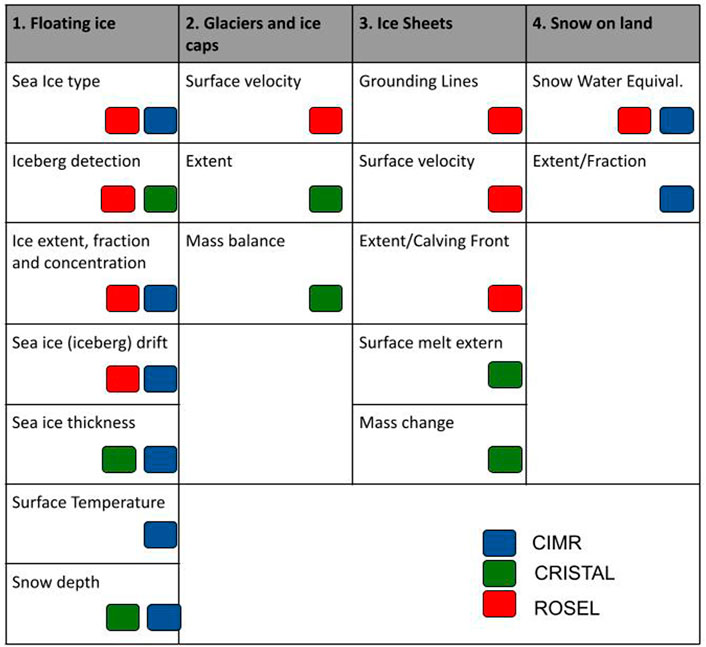
FIGURE 1. High priority environmental parameters identified by the Polar Expert Group (PEGIII) and with color codes, the parameters which can be acquired by each of the polar Copernicus Sentinel Expansion Missions. Blue dots indicate data from CIMR, green dots from CRISTAL, and RED dots from ROSE-L.

This review emphasizes the great potential that the three future polar Copernicus Sentinel Expansion Missions (CIMR, CRISTAL, and ROSE-L) have for the monitoring of the Polar Regions with better resolution and accuracy with respect to the current missions. Moreover, it shows that the three polar missions are required to accommodate the parameters identified by the Polar Expert Group.

3.3 Enhance synergies combining satellite products

Synergies are achievable by combining data from satellite instruments operated at different frequencies/wavelengths, in passive or/and active modes, with different spatio-temporal resolutions, different penetration depths, and thus different sensitivities to the geophysical parameters, and with different impacts of meteorological and environmental conditions (such as cloud coverage and available light) on parameter retrieval.

Table 1 shows the classification of current and potential synergies in Copernicus, which are listed below.

• Eight potential synergies of different types of sensors are presented for land, eight more for ocean and ice and two for biogeochemistry parameters, most of them already demonstrated in the scientific literature. From those potential 18 synergies, only four will be operational in Copernicus by the end of phase 1, the rest are experimental.

• The type of user (intermediate users or end-users land/ocean who can benefit from the new product) is specified, as well as the impact for the users (high, middle, low) of producing these enhanced products. Most of the proposed parameters are appropriate for intermediate users and therefore, will have an important impact for end-users.

• Larger number of similar observations (similar instruments onboard different missions) would improve the measurement uncertainty as well as the temporal resolution.

TABLE 1

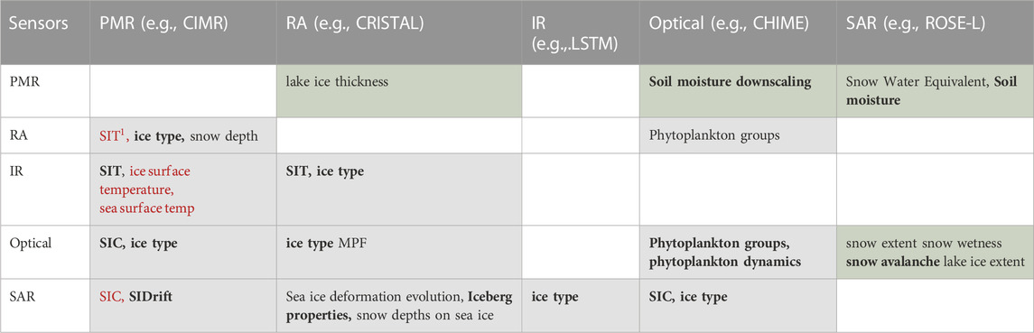
TABLE 1. Matrix of potential synergies that could be put on operation with current and future Copernicus satellites. The synergies mentioned are already tested experimentally. The green boxes are synergies for land applications, light gray for ice and sea applications. Text in red means an operational product in Copernicus phase 1 (2021). Parameters with high impact for intermediate and end-users are marked with bold.

3.4 Recommendation for supporting maritime safety

Shipping routes at high latitudes are increasingly seen as an attractive option, with shorter distances and lower risk of encountering conflict than traditional routes such as via the Suez or Panama Canals, together with an increasingly longer open-water navigation season due to climate change. The Northern Sea Route (NSR) north of Siberia is seeing increasing traffic, particularly with development of Russian oil and natural gas reserves. On the other side of the Arctic, the North West Passages (NWP), through the Canadian Archipelago has more traffic from resupply of settlements along the route, and an increase in mining of natural resources. Other areas, such as the Svalbard Archipelago, Greenland waters, and the Antarctic Peninsula, are experiencing a rise in eco-tourism, with large numbers of vessels traveling to these areas during summer months, and the operating season being stretched earlier and later in the year to periods where sea ice may be encountered. Fishing vessels operate close to, and occasionally in sea ice, over large areas of the Barents, Greenland, and Icelandic Seas in the Arctic, and in the Southern Ocean around Antarctica.

Navigation, and maritime safety, require mapping at high resolution (better than 100 m) and at least daily updating. The increasing volume of available satellite data from different, and sometimes complementary, sensors calls for automatic processing to make full and timely use of the information. Nevertheless, there is still a necessity for quality control and ensuring that the users are given an accurate and reliable evaluation of the ice conditions through ice charts. Most users do not have the necessary experience to safely interpret SAR images, or to decide between a number of scientific products that provide varying levels of conflicting information.

Polar shipping routes cover large areas, and to support activities in these regions improved SAR coverage is necessary. This can be supplied with existing medium resolution sensors such as Sentinel-1 and RCM, but even these at 40–50 m resolution lack the resolution for coastal waters and key straits. C- and X-band frequency SAR, for example, are not optimal for providing information on sea ice deformation features, and for separating sea ice types during summer months. Although there have been extensive scientific investigations into automatic mapping from these over the past 20 years, there are still no robust and reliable techniques that would provide coverage throughout the year, with summer conditions remaining problematic. The combined use of C- and L-band SAR has been demonstrated in research studies to provide improved sea ice type information and iceberg detection, but is not yet widely available and therefore the ROSE-L is seen as essential for safe shipping in Polar Regions.

Greater resolution in SAR wide-swath modes (10 m minimum) is necessary to enable the monitoring of smaller icebergs. Although SAR coverage has increased, and is much improved since International Polar Year (IPY 2007–2009), there is still very sparse information on iceberg climatology, except for the waters around Newfoundland where aerial reconnaissance still takes place. In areas such as the Barents Sea with extensive maritime activity, icebergs are an infrequent but real hazard, yet climatology information is typically 30 years out-of-date. It is unclear whether climate change is increasing the risk, with greater potential for glaciers calving icebergs, or decreasing the risk, due to their faster melting by warm currents and waves.

In addition to the use of different SAR frequency, and increased spatial resolution, sea ice type classification will continue to benefit from additional polarimetric channels. There is still some doubt as to whether dual-polarisation is adequate, and studies have demonstrated that full, or compact, polarimetry has the potential to improve ice type classification.

SAR is the workhorse sensor for effective mapping of sea ice and icebergs for maritime safety and navigation. Synergies between sensors, provide additional information, and resolve ambiguities in interpretation. These can either be through combined use of SAR at different frequencies, such as with C-band Sentinel-1 and L-band ROSE-L mentioned above, or with other types of sensor such as optical or altimetry. Due to sea ice drift, coordination of orbits and ensuring minimal time interval between acquisitions of the different sensors is essential to reduce issues with colocation of the data. This should be prioritised over temporal revisit frequency.

A key issue for microwave sensors is melting, since the penetration depth of radar waves at higher frequencies (X- and C-band) into wet snow is much reduced, hence the radar is blind to the ice structures below the snow. Later in the melt season, extensive melt ponding occurs which causes ambiguities in the interpretation of SAR images, but also with new, featureless very level ice in winter such as found in fjords. During summer months, on the other hand, the maritime activity and corresponding need for accurate information is greatest. Synergies should be investigated with cloud-free optical satellite data as a means of improving classification.

Whilst SAR gives an indication of the sea ice type, and therefore a rough indication as to its thickness, its benefits become clear when combined with other data streams. Experts blend in additional information such as in situ observations, the weather situation and ice drift patterns from the past days, and altimeter-derived sea ice freeboard or thickness to provide additional confirmation and improved labelling of segmented SAR images.

Improved satellite-derived sea ice and iceberg information products will benefit forecast models, which will then have sufficient skill to cover the time intervals between acquisitions.

3.5 Recommendation for data assimilation in ocean ice forecast systems

Today, satellite-derived products are disseminated and assimilated as independent L3 or L4 data products for each variable: independent algorithms at several processing centres process the same L1 data and return independent estimates of variables such as concentration and type. Such collection of higher-level, single-variable products is sub-optimal and causes problems when assimilating them into forecast models. One issue is the inconsistency between data products, especially in the vicinity of sharp gradients such as the ice edge. Another issue is that the spatio-temporal variability of the L1 TB is lost in the daily gridded aggregated products. The hypothesis of Gaussian uncertainties, central to the main Data Assimilation techniques, is broken for the derived data products of sea-ice concentration (SIC) that are bounded between 0% and 100%, which typically cuts off 5% of the signal at high concentrations (inside the ice pack).

Over the past two decades, alternative retrieval methods have been developed to simultaneously retrieve multiple variables and partly overcome the issues described above. An example of a pan-Arctic multivariate retrievals is (Melsheimer et al., 2008) who proposed an integrated retrieval method to derive seven geophysical parameters [SIC and MYI fraction, and a series of ocean and bulk atmosphere variables] and their uncertainties by using an optimal estimation method (OEM). The OEM inverts the satellite simulator of (Wentz and Meissner, 2000)—adapted to icy waters—which can predict the set of multi-frequency PMW TB from the geophysical state of the surface and atmosphere. Several refinements to the OEM method were later proposed by Scarlat et al. (2017), Scarlat, (2018), Scarlat et al. (2020). One advantage of this approach is that the observation uncertainties (of the L1 TB) are now clearly Gaussian. Using a similar satellite simulator but in a 3D variational strategy, Scott et al. (2012) tested the assimilation of L1 TB data and showed its benefit in a limited area along the eastern coast of Canada (mostly FYI). Other attempts using more physically based formulations for the sea-ice emissivities exist (e.g., Burgard et al., 2020) but not at Ku- and Ka-band, the frequencies offering the spatial resolution required by forecast systems.

All these previous attempts clearly indicate the potential for direct assimilation of L1 TB in coupled ocean and sea-ice forecast systems, but also that we should move away from simplified (fixed values) sea-ice emissivities in the satellite simulator. Coincidentally, strategies for dynamic calibration of the sea-ice emissivities (and tie-points) have recently been developed in the SIC processing chains of the EUMETSAT OSI SAF and ESA Climate Change Initiative (CCI) (Lavergne et al., 2019) in order to better capture regional and temporal variations. In particular, they observed and implemented for the first time a parametric curve instead of the classical 100% sea-ice emissivity line between fixed FYI and MYI points.

In principle, the same methodology can also improve the assimilation of ocean surface variables such as sea-surface temperature (SST) and even salinity (SSS).

4 Conclusion and guidance to improve the polar monitoring

The marine and terrestrial environment in the Polar Regions is changing, these entail both challenges and opportunities. Earth Observation has a key role to play in the sustainable development of the region, and information services must be flexible in order to respond to the changing needs and conditions. Importantly, they must provide more information for the Arctic peoples and the wider society, science, private sector and decision makers. Whilst Copernicus offers an impressive range of information services that draw from both satellite and in-situ data, a number of issues with current Copernicus information provision were identified. These include.

• The lack of dialogue between the broader European research community and the Copernicus Services and the Thematic Data Assembly Centers - TACs.

• The disjointed nature of the Arctic observing network, and the data they produce, impacts operational monitoring and hinders the calibration/validation of Copernicus polar products and services.

• New observational technologies are being developed to monitor our environment, however, there is no clear mechanism for their systematic use in the polar regions, or how best to utilise these data streams within Copernicus.

• Data processing latencies and communications bandwidth limitations mean Copernicus has an inability to deliver information near-real time (NRT) to support critical operations such as disaster management and search-and-rescue in the polar regions.

• Lack of synergy in the use of data products coming from different satellite missions, which suggest there are a number of parameters that are not provided using existing capabilities (see Table 1).

In addition to the above mentioned shortcomings our research suggested that improvements to the Copernicus Polar Services could be viewed over different time scales. Suggestions for immediate enhancement, i.e., time scale of less than a year focus on recommendations of easy to achieve goals based on best practices that can be implemented with minimal funding required. These include.

• Improving communications between stakeholders and end-users to better identify the end-users needs.

• Promoting Citizen Science to enhance and increase that amount of in situ data collection that is relevant for the Copernicus Polar Services.

Over the mid to long-term time frame, between 1 and 5 years, opportunities for enhancing polar monitoring under Copernicus activities include.

• Promotion of community-based and local monitoring programmes to provide important information, feedback and in situ data that potentially could fill the gaps and contribute to such areas as climate change, risk management, safety, food- and water security.

• Prioritisation of in-situ measurements for the calibration and validation of the remote sensing data in the Polar Regions through better utilisation of European polar research assets (i.e., stations, ships, aircrafts, and people). As well as establishing closer connections with relevant organisations such as European Polar Board, and international coordinating programmes like Sustaining Arctic Observing Networks (SAON).

• Incorporation of remotely sensed parameters that are not currently being served into Copernicus, for full list see Tables 2.1 and 2.2 in the D3.3 KEPLER Report (https://kepler-polar.eu/deliverables/).

• Consolidation of Arctic-relevant products so that they can all be accessed in a single unified Arctic repository. They are currently scattered among various Copernicus services and non-Copernicus projects (e.g., Copernicus Emergency Management Service (CEMS), CMEMS, Copernicus Land Monitoring Service (CLMS), Copernicus Climate Change Service’s (C3S), ESA-CCI).

• Focus resourses on the collection of in-situ data for Copernicus products that are presently not adequately validated.

• Focus efforts on assimilating new satellite data into the Copernicus NRT forecasting and reanalysis systems. Along with a study of the viability of the assimilation of satellite information at lower processing levels (short term: Level-2 and longer-term: Level-1).

Challenges to overcome in the long term, between the next 5–15 years, for Copernicus Polar Services include.

• Maximise the potential of community-based monitoring. Involving people in monitoring who face the daily challenges and consequences of environmental changes can help in adapting decision making on natural resource management to local realities in a rapidly changing Arctic environment.

• Continuation of the three polar Copernicus Expansion missions (CIMR, CRISTAL, and ROSE-L) are necessary to cover the identified high priority environmental parameters defined by the Polar Expert Group.

• More active role in collecting and managing of in situ data by the Copernicus in situ Component. Focused in situ data will provide a more robust quality assessment of satellite products and improve the geophysical retrieval algorithms.

• Enhanced spatial resolution of sea ice and iceberg data, with a target of 300 m or better, while keeping a wide areal coverage. This is a requirement of the end users, especially from those dedicated to maritime transport.

• Upcoming polar missions should consider the extent of their polar observation hole in the design phase, and thoroughly evaluate the trade-offs required for reducing their extent within the constraints of the mission’s objectives.

• Observing system simulation experiments and (computationally more efficient) quantitative network design studies should be routinely applied in the design of new space missions, the specification of mission requirements and the development of new types of products.

Author contributions

Contributed to conception and design: CG, NH, and JW. Drafted and/or revised the article: All authors. Approved the submitted version for publication: All authors.

Funding

This work has been done under the EU Horizon 2020 Coordination and Support Action (CSA) projecte KEPLER, H2020-SPACE-2018-2020, grant agreement No. 821984, which run from January 2019 to 30 June 2021. The contirbution by AB was further funded by the ESA S5P + Innovation Theme 7 Ocean Colour 532 (S5POC) project (No 4000127533/19/I-NS) and the DFG #268020496-TRR 172 project C03 within the Transregional Collaborative Research Center ArctiC Amplication: Climate Relevant Atmospheric and SurfaCe Processes, and Feedback Mechanisms (AC3).

Acknowledgments

We would like to acknowledge researchers who help somehow on the text: Leif Toudal Pedersen (EoLAB), Steinar Eastwood (MetNo), Signe Aaboe (MetNo), Rune Storvold (NORCE), Jordi Isern (ICM/CSIC), Marcos Portabella (ICM/CSIC). This work is part of the CSIC-PTI TELEDETECT activities and PTI Polar CSIC. This work acknowledges the Severo Ochoa Centre of Excellence accreditation (CEX2019-000928-S).

Conflict of interest

The authors declare that the research was conducted in the absence of any commercial or financial relationships that could be construed as a potential conflict of interest.

Publisher’s note

All claims expressed in this article are solely those of the authors and do not necessarily represent those of their affiliated organizations, or those of the publisher, the editors and the reviewers. Any product that may be evaluated in this article, or claim that may be made by its manufacturer, is not guaranteed or endorsed by the publisher.

References

Ardhuin, F., Aksenov, Y., Benetazzo, A., Bertino, L., Brandt, P., Caubet, E., et al. (2018). Measuring currents, ice drift, and waves from space: The sea surface kinematics multiscale monitoring (SKIM) concept. Ocean. Sci. 14, 337–354. doi:10.5194/os-14-337-2018

CrossRef Full Text | Google Scholar

Aristeidou, M., and Herodotou, C. (2020). Online citizen science: A systematic review of effects on learning and scientific literacy. Citiz. Sci. Theory Pract. 5 (1), 11. doi:10.5334/cstp.224

CrossRef Full Text | Google Scholar

Armitage, T. W. K., Bacon, S., Ridout, A. L., Thomas, S. F., Aksenov, Y., and Wingham, D. J. (2016). Arctic sea surface height variability and change from satellite radar altimetry and GRACE, 2003–2014. J. Geophys. Res. Oceans 121, 4303–4322. doi:10.1002/2015JC011579

CrossRef Full Text | Google Scholar

Bartsch, A., Beck, I., Biskaborn, B., Burba, G., Duguay, C., Grosse, G., et al. (2014). Requirements for monitoring of permafrost in polar regions - a community white paper in response to the WMO Polar Space Task Group. PSTG, 20. doi:10.1594/PANGAEA.847

CrossRef Full Text | Google Scholar

Bartsch, A., Westermann, S., and Strozzi, T. (2021). ESA CCI+ permafrost product validation and algorithm selection report (PVASR), v3.0. ESA. Available at: https://climate.esa.int/media/documents/CCI_PERMA_D2.1_PVASR_v3.0.pdf.

Google Scholar

Burgard, C., Notz, D., Pedersen, L. T., and Tonboe, R. T. (2020). The Arctic Ocean Observation Operator for 6.9 GHz (ARC3O) – Part 1: How to obtain sea ice brightness temperatures at 6.9 GHz from climate model output. Cryosphere 14, 2369–2386. doi:10.5194/tc-14-2369-2020

CrossRef Full Text | Google Scholar

Comiso, J. C., Cavalieri, D. J., Parkinson, C. L., and Gloersen, P. (1997). Passive microwave algorithms for sea ice concentration: A comparison of two techniques. Remote Sens. Environ. 60, 357–384. doi:10.1016/s0034-4257(96)00220-9

CrossRef Full Text | Google Scholar

Dammann, D. O., Eriksson, L. E. B., Jones, J. M., Mahoney, A. R., Romeiser, R., Meyer, F. J., et al. (2019). Instantaneous sea ice drift speed from TanDEM-X interferometry. Cryosphere 13, 1395–1408. doi:10.5194/tc-13-1395-2019

CrossRef Full Text | Google Scholar

Demchev, D., Volkov, V., Kazakov, E., Alcantarilla, P. F., Sandven, S., and Khmeleva, V. (2017). Sea ice drift tracking from sequential SAR images using accelerated-KAZE features. IEEE Trans. Geosc. Remote Sens. 55 (9), 5174–5184. doi:10.1109/TGRS.2017.2703084

CrossRef Full Text | Google Scholar

Dierking, W., and Dall, J. (2008). Sea Ice deformation state from synthetic aperture radar imagery—Part II: Effects of spatial resolution and noise level. IEEE Trans. Geoscience Remote Sens. 46, 2197–2207. doi:10.1109/TGRS.2008.917267

CrossRef Full Text | Google Scholar

Dierking, W., and Dall, J. (2007). Sea-Ice deformation state from synthetic aperture radar imagery—Part I: Comparison of C- and L-band and different polarization. IEEE Trans. Geoscience Remote Sens. 45, 3610–3622. doi:10.1109/TGRS.2007.903711

CrossRef Full Text | Google Scholar

Dierking, W. (2021). “Sea ice and icebergs,” in Maritime surveillance with synthetic aperture radar. Editors G. Di Martino, and A. Iodice (London: The Institution of Engineering and Technology), 173–226. 978-1-78561-601-3.

Google Scholar

Dierking, W., Stern, H. L., and Hutchings, J. K. (2020). Estimating statistical errors in retrievals of ice velocity and deformation parameters from satellite images and buoy arrays. Cryosphere 14, 2999–3016. doi:10.5194/tc-14-2999-2020

CrossRef Full Text | Google Scholar

Eckerstorfer, M., Malnes, E., and Müller, K. (2017). A complete snow avalanche activity record from a Norwegian forecasting region using Sentinel-1 satellite-radar data. Cold Reg. Sci. Technol. 144, 39–51. doi:10.1016/j.coldregions.2017.08.004

CrossRef Full Text | Google Scholar

ESA (2019). Copernicus L-band SAR - mrd 2.0. Available at: https://esamultimedia.esa.int/docs/EarthObservation/Copernicus_L-band_SAR_mission_ROSE-L_MRD_v2.0_issued.pdf.

Google Scholar

European Environment Agency (EEA) (2020). European ground motion service: Service implementation plan and product specification document. Available at: https://land.copernicus.eu/user-corner/technical-library/egms-specification-and-implementation-plan.

Google Scholar

Groom, S., Sathyendranath, S., Ban, Y., Bernard, S., Brewin, R., Brotas, V., et al. (2019). Satellite Ocean colour: Current status and future perspective. Front. Mar. Sci. 6, 485. doi:10.3389/fmars.2019.00485

CrossRef Full Text | Google Scholar

Guneriussen, T., Hogda, K. A., Johnsen, H., and Lauknes, I. (2001). InSAR for estimation of changes in snow water equivalent of dry snow. IEEE Trans. Geoscience Remote Sens. 39 (10), 2101–2108. doi:10.1109/36.957273

CrossRef Full Text | Google Scholar

Hecker, S., Haklay, M., Bowser, A., Makuch, Z., Vogel, J., and Bonn, A. (2018). Citizen science: Innovation in open science, society and policy. London: UCL Press. doi:10.14324/111.9781787352339

CrossRef Full Text | Google Scholar

Hollands, T., and Dierking, W. (2011). Performance of a multi-scale correlation algorithm for the estimation of sea ice drift from SAR images: Initial results. Ann. Glaciol. 52 (57), 311–317. doi:10.3189/172756411795931462

CrossRef Full Text | Google Scholar

Huntemann, M., Heygster, G., Kaleschke, L., Krumpen, T., Mäkynen, M., and Drusch, M., (2014). Empirical sea ice thickness retrieval during the freeze up period from SMOS high incident angle observations. Cryosphere 8 (2), 439–451. doi:10.5194/tc-8-439-2014

CrossRef Full Text | Google Scholar

Itkin, P., Spreen, G., Cheng, B., Doble, M., Girard-Ardhuin, F., Haapala, J., et al. (2017). Thin ice and storms: Sea ice deformation from buoy arrays deployed during N-ICE2015. J. Geophys. Res. Oceans 122, 4661–4674. doi:10.1002/2016JC012403

CrossRef Full Text | Google Scholar

Ivanova, N., Johannessen, O. M., Pedersen, R. T., and Tonboe, R. T. (2014). Retrieval of arctic sea ice parameters by satellite passive microwave sensors: A comparison of eleven sea ice concentration algorithms. IEEE Trans. Geosci. Remote 52, 7233–7246. doi:10.1109/TGRS.2014.2310136

CrossRef Full Text | Google Scholar

Kaleschke, L., Tian-Kunze, X., Maaß, N., Mäkynen, M., and Drusch, M. (2012). Sea ice thickness retrieval from SMOS brightness temperatures during the Arctic freeze-up period. Geophys. Res. Lett. 39 (5). doi:10.1029/2012GL050916

CrossRef Full Text | Google Scholar

Karvonen, J. (2014). A sea ice concentration estimation algorithm utilizing radiometer and SAR data. Cryosphere 8, 1639–1650. doi:10.5194/tc-8-1639-2014

CrossRef Full Text | Google Scholar

Kern, S., Lavergne, T., Notz, D., Pedersen, L. T., and Tonboe, R. (2020). Satellite passive microwave sea-ice concentration data set inter-comparison for Arctic summer conditions. Cryosphere 14, 2469–2493. doi:10.5194/tc-14-2469-2020

CrossRef Full Text | Google Scholar

Kilic, L., Prigent, C., Jimenez, C., and Donlon, C. (2021). Technical note: A sensitivity analysis from 1 to 40 GHz for observing the Arctic Ocean with the Copernicus imaging microwave radiometer. Ocean. Sci. 17, 455–461. doi:10.5194/os-17-455-2021

CrossRef Full Text | Google Scholar

Korosov, A. A., and Rampal, P. (2017). A combination of feature tracking and pattern matching with optimal parametrization for sea ice drift retrieval from SAR data. Remote Sens. 9, 258. doi:10.3390/rs9030258

CrossRef Full Text | Google Scholar

Kræmer, T., Johnsen, H., Brekke, C., and Engen, G. (2018). Comparing SAR-based short time-lag cross correlation and Doppler-derived sea ice drift velocities. IEEE Trans. Geosc. Remote Sens. 56 (9), 1898–1908. doi:10.1109/TGRS.2017.2769222

CrossRef Full Text | Google Scholar

Kroisleitner, C., Bartsch, A., and Bergstedt, H. (2018). Circumpolar patterns of potential mean annual ground temperature based on surface state obtained from microwave satellite data. Cryosphere 12, 2349–2370. doi:10.5194/tc-12-2349-2018

CrossRef Full Text | Google Scholar

Lavergne, T., Eastwood, S., Teffah, Z., Schyberg, H., and Breivik, L.-A. (2010). Sea ice motion from low resolution satellite sensors: An alternative method and its validation in the arctic. J. Geophys. Res. 115, C10032. doi:10.1029/2009JC005958

CrossRef Full Text | Google Scholar

Lavergne, T., Piñol Solé, M., Down, E., and Donlon, C. (2021). Towards a swath-to-swath sea-ice drift product for the Copernicus Imaging Microwave Radiometer mission. Cryosphere 15, 3681–3698. doi:10.5194/tc-15-3681-2021

CrossRef Full Text | Google Scholar

Lavergne, T., Sørensen, A. M., Kern, S., Tonboe, R., Notz, D., Aaboe, S., et al. (2019). Version 2 of the EUMETSAT OSI SAF and ESA CCI sea-ice concentration climate data records. Cryosphere 13, 49–78. doi:10.5194/tc-13-49-2019

CrossRef Full Text | Google Scholar

Laxon, S. W., Giles, K. A., Ridout, A. L., Wingham, D. J., Willatt, R., Cullen, R., et al. (2013). CryoSat-2 estimates of Arctic sea ice thickness and volume. Res. Lett. 40, 732–737. doi:10.1002/grl.50193

CrossRef Full Text | Google Scholar

Lewandowski, E., Caldwell, W., Elmquist, D., and Oberhauser, K. (2017). Public perceptions of citizen science. Citiz. Sci. Theory Pract. 2 (13), 3–9. doi:10.5334/cstp.77

CrossRef Full Text | Google Scholar

Lfritz, S., Dias, E., et al. (2016). Supporting earth-observation calibration and validation: A new generation of tools for crowdsourcing and citizen science. IEEE Geosci. Magaz 4, 38–50. doi:10.1109/MGRS.2015.2498840

CrossRef Full Text | Google Scholar

Lievens, H., Demuzere, M., Marshall, H. P., Reichle, R. H., Brucker, L., Brangers, I., et al. (2019). Snow depth variability in the Northern Hemisphere mountains observed from space. Nat. Commun. 10, 4629. doi:10.1038/s41467-019-12566-y

PubMed Abstract | CrossRef Full Text | Google Scholar

Lindsay, R. W., and Stern, H. L. (2003). The RADARSAT geophysical processor system: Quality of Sea Ice trajectory and deformation estimates. J. Atmos. Ocean. Technol. 20, 1333–1347. doi:10.1175/1520-0426(2003)020<1333:trgpsq>2.0.co;2

CrossRef Full Text | Google Scholar

Losa, S., Soppa, M. A., Dinter, T., Wolanin, A., Brewin, R. J. W., Bricaud, A., et al. (2017). Synergistic exploitation of hyper- and multi-spectral precursor Sentinel measurements to determine phytoplankton functional types (SynSenPFT). Front. Mar. Sci. 4, 203. doi:10.3389/fmars.2017.00203

CrossRef Full Text | Google Scholar

Ludwig, V., Spreen, G., Haas, C., Istomina, L., Kauker, F., and Murashkin, D. (2019). The 2018 North Greenland polynya observed by a newly introduced merged optical and passive microwave sea-ice concentration dataset. Cryosphere 13, 2051–2073. doi:10.5194/tc-13-2051-2019

CrossRef Full Text | Google Scholar

Martínez, J., Gabarró, C., Turiel, A., González-Gambau, V., Umbert, M., Hoareau, N., et al. (2022). Improved BEC SMOS arctic Sea Surface salinity product v3.1. Earth Syst. Sci. Data 14, 307–323. doi:10.5194/essd-14-307-2022

CrossRef Full Text | Google Scholar

Melsheimer, C., Heygster, G., and Pedersen, L. T. (2008). “Integrated retrieval of surface and atmospheric parameters over the Arctic from AMSR-E satellite microwave radiometer data using inverse methods,” in IGARSS 2008-2008 IEEE International Geoscience and Remote Sensing Symposium, Boston, 07-11 July 2008 (IEEE), IV, 4–986.

CrossRef Full Text | Google Scholar

Nagler, T., and Rott, H. (2000). Retrieval of wet snow by means of multitemporal SAR data. IEEE Trans. Geoscience Remote Sens. 38 (2), 754–765. doi:10.1109/36.842004

CrossRef Full Text | Google Scholar

Nordbeck, O., Duchossois, G., Kohlhammer, G., Andersson, E., Diehl, T., Dinessen, F., et al. (2021). User requirements for a Copernicus polar observing system– phase 3 report - towards operational products and services. Luxembourg: Publications Office of the European Union. 978-92-76-34378-3. doi:10.2889/90647

CrossRef Full Text | Google Scholar

Obu, J., Westermann, S., Barboux, C., Bartsch, A., Delaloye, R., Grosse, G., et al. (9999). ESA permafrost climate change initiative (Permafrost_cci): Permafrost version 3 data products. Centre Environ. Data Analysis. 2021-12-21. Available at: http://catalogue.ceda.ac.uk/uuid/8239d5f6263f4551bf2bd100d3ecbead.

Google Scholar

Oelker, J., Losa, S. N., Richter, A., and Bracher, A. (2022). TROPOMI-retrieved underwater light attenuation in three spectral regions in the ultraviolet and blue. Front. Mar. Sci 9, 787992. doi:10.3389/fmars.2022.787992

CrossRef Full Text | Google Scholar

IPCC (2019). in IPCC special report on the ocean and cryosphere in a changing climate. Editors H.-O. Pörtner, D. C. Roberts, V. Masson-Delmotte, P. Zhai, M. Tignor, E Poloczanskaet al.

Google Scholar

Prandi, P., Poisson, J.-C., Faugère, Y., Guillot, A., and Dibarboure, G. (2021). Arctic sea surface height maps from multi-altimeter combination. Earth Syst. Sci. Data 13, 5469–5482. doi:10.5194/essd-13-5469-2021

CrossRef Full Text | Google Scholar

Ray, C., Martin-Puig, C., Clarizia, M. P., Ruffini, G., Dinardo, S., Gommenginger, C., et al. (2015). SAR altimeter backscattered waveform model. IEEE Trans. Geoscience Remote Sens 53, 911–919. doi:10.1109/tgrs.2014.2330423

CrossRef Full Text | Google Scholar

Ricker, R., Hendricks, S., Kaleschke, L., Tian-Kunze, X., King, J., and Haas, C. (2017). A weekly Arctic sea-ice thickness data record from merged CryoSat-2 and SMOS satellite data. Cryosphere 11, 1607–1623. doi:10.5194/tc-11-1607-2017

CrossRef Full Text | Google Scholar

Robinson, I. S. (2004). Measuring the Oceans from Space: The principles and methods of satellite oceanography. Berlin: Springer, 669.

Google Scholar

Rott, H., Yueh, S., Cline, D. W., Duguay, C., Essery, R., Haas, C., et al. (2010). Cold regions hydrology high-resolution observatory for snow and cold land processes. IEEE Trans. geoscience remote Sens. 99, 1–10. doi:10.1109/JPROC.2009.2038947

CrossRef Full Text | Google Scholar

Ryu, J.-H., Han, H.-J., Cho, S., Park, Y-J., and Ahn, Y-H. (2012). Overview of geostationary ocean color imager (GOCI) and GOCI data processing system (GDPS). Ocean. Sci. J. 47 (3), 223–233. doi:10.1007/s12601-012-0024-4

CrossRef Full Text | Google Scholar

Salomonson, V. V., and Appel, I. (2004). Estimating fractional snow cover from MODIS using the normalized difference snow index. Remote Sens. Environ. 89 (3), 351–360. doi:10.1016/j.rse.2003.10.016

CrossRef Full Text | Google Scholar

Sathyendranath, S., Brewin, R. J. W., Brockmann, C., Brotas, V., Calton, B., Chuprin, A., et al. (2019). An Ocean-colour time series for use in climate studies: The experience of the ocean-colour climate change initiative (OC-CCI). Sensors 19, 4285. doi:10.3390/s19194285

PubMed Abstract | CrossRef Full Text | Google Scholar

Scarlat, R. C., Heygster, G., and Pedersen, L. T. (2017). Experiences with an optimal estimation algorithm for surface and atmospheric parameter retrieval from passive microwave data in the Arctic. IEEE J. Sel. Top. Appl. Earth Observations Remote Sens. 10 (9), 3934–3947. doi:10.1109/jstars.2017.2739858

CrossRef Full Text | Google Scholar

Scarlat, R. C. (2018). Improving an optimal estimation algorithm for surface and atmospheric parameter retrieval using passive microwave data in the Arctic Universität Bremen. Available at: http://nbn-resolving.de/urn:nbn:de:gbv:46-00106738-16.

Google Scholar

Scarlat, R. C., Spreen, G., Heygster, G., Huntemann, M., Paţilea, C., Toudal Pedersen, L., et al. (2020). Sea Ice and atmospheric parameter retrieval from satellite microwave radiometers: Synergy of AMSR2 and SMOS compared with the CIMR candidate mission. J. Geophys. Res. Oceans 125. doi:10.1029/2019JC015749

CrossRef Full Text | Google Scholar

Scott, K. A., Buehner, M., Caya, A., and Carrieres, T. (2012). Direct assimilation of AMSR-E brightness temperatures for estimating Sea Ice“, concentration. Mon. Wea. Rev. 140, 997–1013. doi:10.1175/MWR-D-11-00014.1

CrossRef Full Text | Google Scholar

Shirk, J. L., Ballard, H. L., Wilderman, C. C., Phillips, T., Wiggins, A., Jordan, R., et al. (2012). Public participation in scientific research: A framework for deliberate design. Ecol. Soc. 17 (2), 29. doi:10.5751/ES04705-170229

CrossRef Full Text | Google Scholar

Silva, T. A. M., Bigg, G. R., and Nicholls, K. W. (2006). Contribution of giant icebergs to the Southern Ocean freshwater flux. J. Geophys. Res. 111 (C3), C03004. doi:10.1029/2004JC002843

CrossRef Full Text | Google Scholar

Tilstone, G., Dall'Olmo, G., Hieronymi, M., Ruddick, K., Beck, M., Ligi, M., et al. (2020). Field intercomparison of radiometer measurements for ocean colour validation. Remote Sens. 12 (10), 1587. doi:10.3390/rs12101587

CrossRef Full Text | Google Scholar

Trofaier, A. M., Westermann, S., and Bartsch, A. (2017). Progress in space-borne studies of permafrost for climate science: Towards a multi-ECV approach. Remote Sens. Environ. 203, 55–70. doi:10.1016/j.rse.2017.05.021

CrossRef Full Text | Google Scholar

Weiss, J. (2013). Drift, deformation, and fracture of Sea Ice: A perspective across scales. Germany: Springer Briefs in Earth Sciences”. doi:10.107/978-94-007-6202-2

CrossRef Full Text | Google Scholar

Wentz, F. J., and Meissner, T. (2000). “AMSR ocean algorithm theoretical basis document, version 2” in Remote Sensing Systems (Santa Rosa, CA). Available at: https://eospso.gsfc.nasa.gov/sites/default/files/atbd/atbd-amsr-ocean.pdf.

Google Scholar

Zwally, H. J., Yi, D., Kwok, R., and Zhao, Y. (2008). ICESat measurements of Sea Ice freeboard and estimates of Sea Ice thickness in the weddell sea. J. Geophys. Res. 113 (C2), C02S15. doi:10.1029/2007JC004284

CrossRef Full Text | Google Scholar