Machine learning for efficient segregation and labeling of potential biological sounds in long-term underwater recordings

1 Introduction

The technological advances in Passive Acoustic Monitoring (PAM) underwater devices in recent years have enormously increased the amount of marine acoustic data available. Studies carried out using these data typically focus on a single or a limited number of species, mainly concentrating on taxa at the top of the food chain (Stowell, 2022; Rubbens et al., 2023). Archived long-term data, however, contain a great diversity of other sounds, most of which remain to date unidentified. Interest in studying these sounds has grown in recent years, as they can serve as a proxy for biodiversity or ecosystem health (Desiderà et al., 2019; Bolgan et al., 2020; Di Iorio et al., 2021; Parsons et al., 2022).

Sound events can inform animals about their surroundings (Au and Hastings, 2008). This can either come in the form of biotic associated sounds from predators, prey, or conspecific, or in the form of geophonic sounds that can contain information about habitat quality or provide navigational cues (Mooney et al., 2020; Schoeman et al., 2022). Since any sound event could potentially carry information about an organism’s environment, characterizing and quantifying unknown sound events can be used to characterize and understand soundscapes. Soundscape characterization has been done by detecting certain acoustic events of relevance, such as animal vocalizations or anthropogenic sounds, and quantifying their temporal patterns, relationships, or proportions (Havlik et al., 2022; Schoeman et al., 2022). This provides knowledge on the local acoustic community and it can be used as a proxy for biodiversity and ecosystem health. Soundscape characterization by isolating acoustic events can also be done with sounds from an unknown source, as long as they can be detected and classified. Finding, reporting, and understanding the patterns of unidentified sounds is of significant benefit to the assessment of underwater soundscapes. This can then help raise awareness and inform policymakers on the health status of an ecosystem and how best to tackle conservation or noise mitigation measures (Parsons et al., 2022).

Some sound sources present diurnal, celestial, seasonal and annual patterns, especially studied for biological sources (Staaterman et al., 2014; Nedelec et al., 2015; Schoeman et al., 2022). For example, certain fish species are known to vocalize during dusk and dawn (Parsons et al., 2016). Therefore, some sources could eventually be assigned to certain sound events by an exclusion procedure taking into account their spatio-temporal patterns, but to do this larger scales than the ones that can be covered in one study/area are necessary. Therefore, a database of unidentified sounds is, in some ways, as important as one for known sources (Parsons et al., 2022); as the field progresses, new unidentified sounds will be collected, and more unidentified sounds can be matched to species. Therefore, documenting these sounds before they are identified provides a baseline for their presence and Supplementary Material for later source identification. This is especially applicable in areas where very little sound sources are clearly described.

However, studying unknown sounds is a challenging task, as it is difficult to find sound events in long-term recordings when one does not know which events to expect. Unidentified sounds might be, or might not be, of importance for the marine fauna. Yet before deciding that a certain sound is relevant, a considerable time investment in the manual screening of the acoustic recordings is necessary, and this can still sometimes be inconclusive (Wall et al., 2014). In the marine environment, this task is even more complicated as biological sounds of interest are often sparse-occurring (Stowell et al., 2015), non-continuous or rare (Looby et al., 2022). Because of the amount of generated PAM data, there is interest in having this process automatized. Several studies suggest that using deep learning is a promising solution (Stowell, 2022). In these studies, the detection and classification are often applied to segmented data, where long recordings are split into equal-sized overlapping windows, and then a binary output algorithm is used to detect the possible sound events (Stowell et al., 2015). Afterwards, the selected windows are run through a classifier where they are assigned a call type, or further discarded as noise. However useful this approach can be, it has its limitations. For example, it is complicated to detect and classify signals of different lengths, or to deal with signals overlapping in time in different frequency bands. When looking for unidentified sounds, these considerations are key, as there are no predefined frequency bands, frequency patterns or event duration to focus on.

Here we propose a method to detect and categorize sound events in long-term recordings. The method concept is inspired by the analysis process of human annotators when screening for unidentified sounds. Human annotators look first at the temporal-spectral shape in a spectrogram, the duration, and the frequency limits to assign certain sounds to a specific species. The sounds are then usually annotated by drawing bounding boxes around them in the time-frequency domain, namely in a spectrogram. Human annotators first screen a lot of hours of recordings before deciding which sound groups can be considered, and only after that are labels assigned to the selected sounds. Therefore, following the same strategy, we propose to use of one of the newest computer vision algorithms for object detection YOLOv8 (Jocher et al., 2023), to detect all the possible sound events on a spectrogram using transfer learning.

Supervised deep learning models such as the proposed detection model (YOLOv8) are known to need large amounts of annotated data to achieve good performances. Hence, to reduce the human annotation effort needed to generate a first dataset to train the model, we propose an active learning approach, where the model selects the files with more diversity of sounds to be manually annotated. We then compare the results with a random selection of files for annotation. To test the robustness of the model to unseen data, and to investigate the possible generalization of the model to detect acoustic events in any underwater environment, the obtained models are tested on two datasets: 1) a test set recorded in the Belgian Part of the North Sea (BPNS) as part of the LifeWatch Broadband Acoustic Network (Parcerisas et al., 2021), and 2) test set of freshwater acoustic recordings collected in 4 major European rivers.

The detection model can then be used to detect sound events in new data. The obtained detections could already be directly used to speed up manual annotations, but they can also be used to further cluster these sound events into sound types and explore the acoustic environment. To this aim, all the detected events are converted into a multidimensional embedding space using another pre-trained deep learning model, which has been trained on a large dataset of diverse bioacoustic data. We then use these embeddings to cluster all the detections in an unsupervised way. This approach enables an initial analysis of the existing sound types within a specific dataset. Through a manual review of the clusters, sound labels can be assigned to them if considered appropriate. Once these clusters are defined and revised, we analyze the obtained temporal patterns and the new sound categories discovered. We showcase this second part of the methodology in a short deployment spanning 10 days in one location of the BPNS.

2 Materials and methods

2.1 General concept flow

The presented methodology is a new approach to discover sound types of a relatively unstudied environment while reducing human annotation and labeling time, providing insights on the spatio-temporal patterns of the discovered sounds leading to potential clues on sound origins.

The general idea of the proposed methodology is to first detect all the potentially relevant underwater acoustic events, regardless of their sound type, using an automated method. Next, the detected events are converted to a multidimensional embedding space and then clustered into different classes. The clusters are then manually revised by checking 10 events per cluster. Finally, the temporal patterns of the obtained clusters are plotted to assist in the identification of the source of each sound type (cluster) and to already provide insight on the soundscape dyamics. A general schematic of the entire process can be seen in Figure 1.

Figure 1

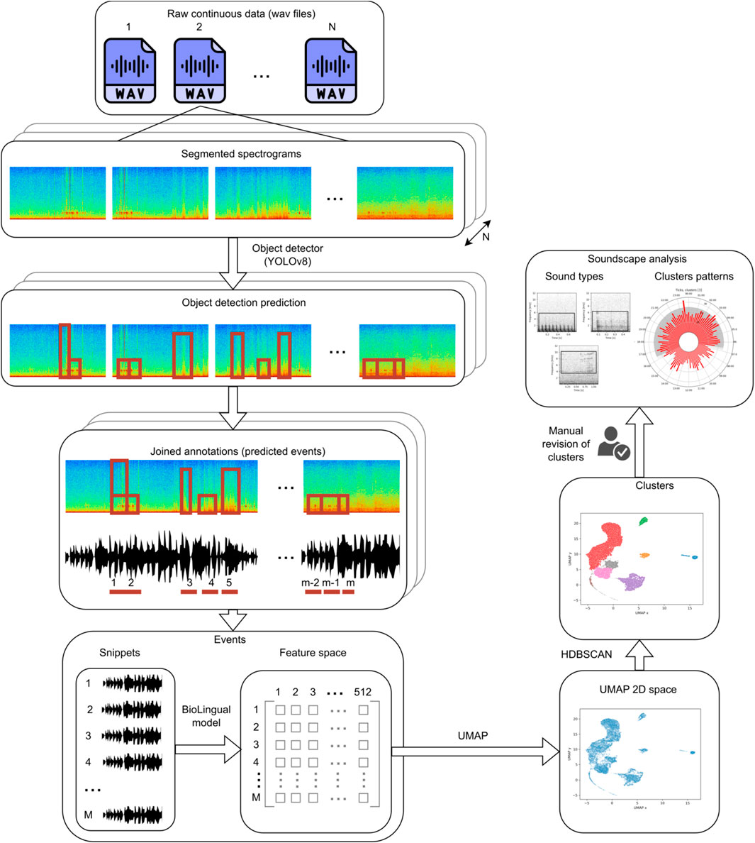
Figure 1. Flow of the proposed methodology. N is the number of wav files to analyze. m is the number of detections in one wav file after joining. M is then the total number of annotations within the N wav files.

For the event detection, because we want to allow for multiple events happening simultaneously in different frequency bands, this detection is performed in the spectro-temporal space using an object detector (YOLOv8) (Jocher et al., 2023) from computer vision. Therefore, the recordings needed segmentation and transformation into images, in order to be ingested in the model. This process is explained in Section 2.4. To account for the continuity of the data, these segments are overlapping. Therefore, the predictions from the object detector need to be merged afterwards to avoid double detections. This is explained in Section 2.5.2. We will refer to the model predictions once they are already joined as sound event detections from now on. Although YOLOv8 is pre-trained, specialization for the task at hand is needed, so the model needs to be re-trained (see Section 2.5.1). This requires a human selection of areas in the spectrogram that are potentially interesting sounds, which is a time-consuming task (see Section 2.3 for details on how these areas are selected). We will refer to this process as human annotation throughout the manuscript. To increase efficiency of this process we propose an active learning approach where audio files are selected that could enrich the database of human annotations most. To this end, suitable metrics are proposed. This process is described in Section 2.6, and it is compared to the random selection of files. The performance of the object detector is tested on two independent manually annotated datasets: an extensive dataset from the BPNS (see Section 2.4.3) and a dataset from freshwater recordings (see Section 2.4.4).

Once all the overlapping predictions are merged, using the start and end time of each sound detection the raw waveform snippet is extracted and filtered to the predicted frequency band (frequency limits predicted by the model). Each snippet is then converted to a multidimensional embedding space using the pre-trained model BioLingual. The obtained features are next reduced to a smaller feature space using UMAP to deal with the curse of dimensionality, and the reduced feature space is clustered using HDBSCAN. The obtained clusters are then manually revised to assign them a label and a possible source (from now on, labeling), and their temporal patterns are analyzed. This process is explained in Section 2.7, and it is performed as a showcase on data from continuous recordings spanning 10 days.

2.2 The datasets

2.2.1 BPNS Data

The audio data were selected from the LifeWatch Broadband Acoustic Network (Parcerisas et al., 2021), implementing RESEA 320 recorders (RTSys, France) together with Colmar GP1190M-LP hydrophones (Colmar, Italy, sensitivity: 180 dB/V re 1μPa, frequency range −3 dB: 10 Hz to 170 kHz), attached to steel mooring frames at 1 m above the sea bottom, with no moving parts. The locations of data collection within the BPNS are displayed in Figure 2 and the deployment periods per station are summarized in Supplementary Table S1. Each deployment was manually screened to decide the period where the data were valid, considering clipping, instrument noise and failure of the recorder. The files considered in this study were all the files falling inside the valid period of a deployment and had less than 1E-6 percentage of data points clipping. All the files were between 5 and 10 min long, depending on the deployment.

Figure 2

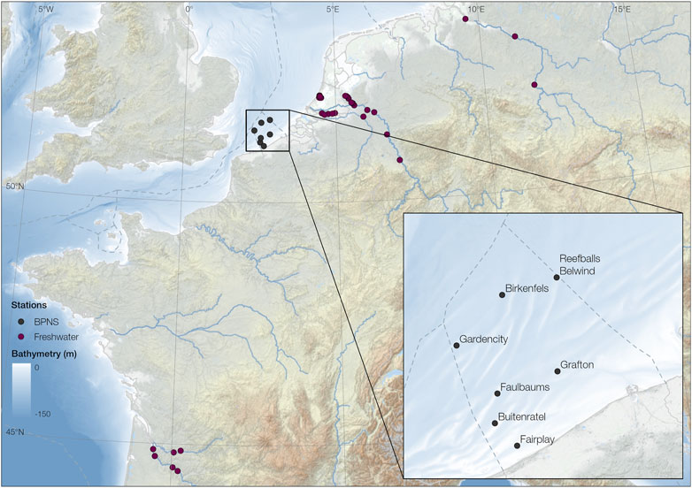
Figure 2. Locations where the sound was acquired, for both the BPNS and the freshwater datasets. Area zoomed to the BPNS with the corresponding station names. Data used from EMODnet Bathymetry Consortium (2018) and GEBCO Compilation Group (2022).

2.2.2 Freshwater Data

To further evaluate the robustness of the detection algorithms the model was tested on an extra test set recorded in a variety of freshwater habitats across Europe. The locations of data collection within Europe are displayed in Figure 2. These habitats included ditch, pond, medium river, large river, and 4 very large European rivers with varying characteristics. The total dataset included 42 different deployments, each at a different location, recorded with two different instruments. On one side, 28 deployments were conducted using SoundTrap 300 STD hydrophones (Ocean Instruments NZ, sensitivity: 176.6 dB re: 1 μPa V⁻¹, frequency range −3 dB 20 Hz to 60 kHz), suspended between an anchor and sub-surface buoy 50 cm above the sediment. The other 14 deployments were recorded using Hydromoth hydrophones (Open Acoustic Devices, unknown calibration specs) (Lamont et al., 2022), attached to a steel frame 20 cm above the sediment. A detailed summary of all the considered deployments can be found in the Supplementary Material Supplementary Table S2.

2.3 Manual annotation on audio files using RavenPro

Manually annotating sounds (drawing bounding boxes around acoustic events in the spectro-temporal space) is a time and human labor-intensive task. This is especially the case when a lot of sounds have to be annotated, and when one does not know what sounds to look for, because the whole bandwidth needs to be screened. In this study we focused on a broad frequency band to include benthic invertebrate, fish and some marine mammal sounds. Invertebrate sounds are characterized by a wide bandwidth and very short duration compared to fish sounds (Minier et al., 2023). This difference in duration and bandwidth poses a challenge during annotation and description of the sounds.

As ground truth to train and test the sound event detection model, wav files were manually annotated using Raven Pro version 1.6.4 (K. Lisa Yang Center for Conservation Bioacoustics at the Cornell Lab of Ornithology, 2023). The software settings were configured to visualize a window duration of 20 s with frequencies ranging from 0 to 12 kHz. To facilitate optimal visual representation, the selected color scale was “Grayscale”, and the spectrograms were generated with a Hann window with 2048 fft bins and a hop size of 164 samples (same parameters than the ones used afterwards to convert the data into images to input to the model). Spectro-temporal bounding boxes were meticulously hand-drawn to accurately capture the contours of the corresponding audio signals as observed in the spectrogram.

Because of the subjectivity of annotating sound events, some rules were decided about how to label events. The first requirement for an event to be logged was that it was both acoustically and visually salient. Therefore, sounds perceived as “background” were not annotated. This included ambient sound but also long, continuous sounds not salient according to subjective human perception. Deciding if a sequence of sound events was a “sentence” or separate individual sounds was done following the subjective criteria of whether the events were perceived to be coming from the same sound source or not, focusing on the continuity of the sound. Abrupt frequency jumps were considered an indication of the start of a different event. Events happening simultaneously at the same time with the same rhythm in different frequency bands were annotated as a single event. In case of doubt, a separate box was always added.

2.4 Data preparation for object detector

The object detector (YOLOv8) is based on visual detections of the sound events. Therefore, the data were processed into spectrograms using overlapping windows longer than the expected sound events of interest. Deciding the parameters to generate spectrograms is a critical step. All these parameters are context-specific and should be chosen in a way that the foreground sounds are contrasting the background in a well-defined and sharp way. The chosen parameters for this context situation are specified in Table 1. Once the spectrograms were generated, they were normalized to the [1, 99] % percentiles after converting to dB, and a spectral high pass filter at 50 Hz was applied to exclude flow noise. Finally, the spectrograms were converted first to gray scale, where white is 0 and black 1 and then converted to RGB using the colorscale ‘jet’ provided by the package matplotlib (python). This step was done because the pre-trained YOLOv8 model was trained on RGB images. Data were processed using the scripts available at https://github.com/lifewatch/sound-segregation-and-categorization, and Raven annotations were converted into the YOLOv8 format for each chunk. An example of several input images with their corresponding annotations is shown on Figure 3.

Table 1

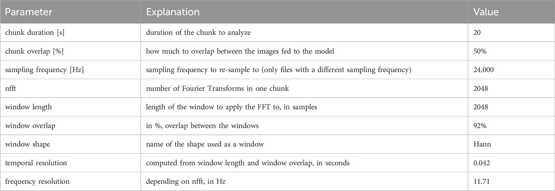
Table 1. Settings used to generate the spectrograms for the YOLOv8 model.

Figure 3

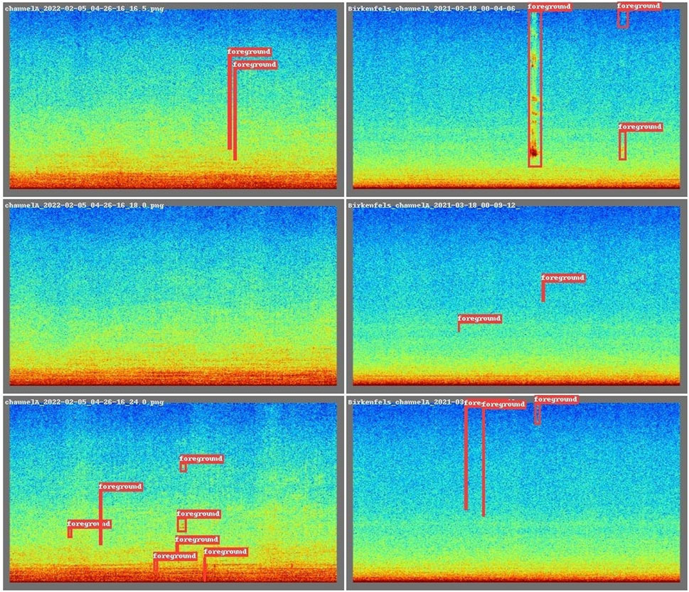
Figure 3. Example of labeled sounds from the unidentified sounds Dataset when colored to RGB values. Each rectangle represents 20 s in the x-axis and 12,000 Hz in the y-axis.

For manual annotations (not model detections), the column SNR NIST Quick (db) of Raven Pro was added as a proxy for the signal to noise ratio (SNR) of the event, to provide a more objective threshold to include an event or not. This was done because human annotations of sound events are not always consistent (Leroy et al., 2018; Nguyen Hong Duc et al., 2021), and “the accuracy of a trained model heavily depends on the consistency of the labels provided to it during training” (Bagherinezhad et al., 2018). Therefore, the post-annotation filtering of SNRs provided a less subjective criteria on whether to add or not an annotation to training or test sets. With this idea, box-annotations with a SNR NIST Quick (db) lower than 10 dB were discarded. For both manual annotations and model detections, all events shorter than 1 pixel in temporal resolution (shorter than 0.085 s) were also removed before the reshaping.

2.4.1 Initial training set

For the initial training set, approximately 1.5 h were used from the Birkenfels station, recorded the 18th of March of 2021, from midnight to 1:30a.m. The annotations were carried out by expert E.S. After processing the raw data, the training data consisted of 556 images in RGB of a size of 1868 × 1,020 pixels, representing 20 s each. From the 556 images, 14 had no annotation (background images). In total there were 1,595 annotations, from which 1,532 complied with the SNR and minimum duration criteria. This was chosen as a representative starting scenario, where the available annotations from a lab are consecutive files from one location.

2.4.2 Pool of data for selecting additional training samples using active learning

A pool of the data was created to avoid predicting the entire dataset at every active learning iteration, which was computationally not feasible. The unlabeled pool for active learning was selected in a stratified fashion considering season, station, moment of the day and Moon phase. Season included the four different seasons, moment of the day considered twilight, night and day, station consisted of the seven different stations of LifeWatch Broadband Acoustic Network, and Moon phase included new, full, growing and decreasing Moon states. The python package Skyfield (Rhodes, 2019) was used to assign the environmental variables to each wav file. Seven files were randomly selected per available combination from all the available wav files of all the recordings, excluding all the files that had been selected for the training set, leading to a total of 1,005 wav file (126.5 h).

2.4.3 BPNS test set

The BPNS test set consisted of a stratified selection of files from the LifeWatch Broadband Acoustic Network. The selection strategy was the same than the one for the unlabeled pool but selecting 1 file per possible combination of environmental variables instead of 7, and excluding all the files from the unlabeled pool and from the training set. The test set was independent of the training set, but it did overlap with the training set regarding location, season and environmental conditions. The final selection consisted of 145 wav files, a total of approximately 18 h. The audio files were processed the same way than the training set, leading to a dataset of 6,342 images. The annotations were carried out by independent annotators K.M and O.S., each annotating half of the test set. The annotations were manually checked using a model-assisted approach to speed up the process. We used the model obtained from training using only the initial training set (Model Base) to predict the files. Then, the human annotator went through all the files, adjusting detections and modifying the boxes boundaries when necessary. Only the manual annotations complying with the selection criteria were used for evaluation.

2.4.4 Freshwater test set

The freshwater test set was also selected for evaluation of the model from all the freshwater data in a stratified way considering water type and moment of day. Moment of day included day, night and civil twilight. The stratified selection was run using the same approach than for the BPNS test set. 24 files of 5 min were selected, from which 21 were recorded with SoundTrap and 3 using Hydromoth. The freshwater test set was annotated by expert K.V.

2.5 Object detector model

2.5.1 Training

The pre-trained YOLOv8n (nano) model was used as an initialization, which was initially trained on the Common Objects in Context (COCO) images dataset (Lin et al., 2015). First this model was re-trained on the initial training set of spectrogram images. From now on we will refer to this model as the Model Base.

For all the training runs, the initialization was kept to the YOLOv8 nano weights. The initial training set was split for training and validation using a K-fold strategy with 3 folds (6 different full files were kept for validation for each model). This led to 3 different Model Base.

For each training round, data were fed into the YOLOv8n model and trained for 200 epochs, with batch size 32. The YOLOv8 model incorporates several data augmentation techniques. The augmentation techniques for mix-up, copy-paste, mosaic, rotation, shear, perspective and scale were deactivated for the re-training and the prediction on new data because they did not represent realistic scenarios in the case of object detection in spectrograms of underwater sounds, and therefore they were not expected to create any advantageous for spectrograms, or could even be detrimental. The rest of the augmentation techniques were kept as the default values. The Intersection Over Union (iou) was set to 0.3 for validation evaluation, and the images were resized to 640 × 640 pixels. The rest of the parameters were kept as the default values.

2.5.2 Joining predictions: from segmented images to continuous audio

We used a minimum confidence of 0.1 for all the predictions. This is the default value used by YOLOv8 for validating the model. Because of the 50% overlap between two consecutive images, some model predictions would be repeated when joined as a continuous audio file. Therefore, we first joined all boxes that had a 50% overlap or more, keeping the largest boundaries resulting from the union of the two boxes. The confidence of the resulting box was assigned to the maximum of the box. The pseud-code to join the boxes is shown in Supplementary Algorithm S1.

2.5.3 Evaluation

The evaluation was done once the detections were already joined. When analyzing sounds using an object detector for unknown sounds, the evaluation metrics are not straight forward. The sound events selected in the ground truth are subjectively split into units or joined, according to the best criteria of the human annotator. Sound events occurring simultaneously in different frequency bands can be considered two different sounds or the same sound, and marked accordingly, but all these options should be considered valid when evaluating the model.

To compute the True Positives, each detection d was compared with all the manual annotations starting and ending between (d_{start_time} - 5) seconds and (d_{end_time} + 5 s). 5 s was chosen as the longest detections were set to 10 s. This selection was done for computational efficiency. For the comparison, the iou was computed between the detection and all the manual annotations within the respective time window. If any iou was greater than 0.3, the detection was marked as a true positive. Detections without an iou value greater than 0.3 were considered false positives. Manual annotations not exceeding an iou of 0.3 for any prediction were considered false negatives. From true positives, false positives and false negatives, we computed recall, precision and F1 metrics.

To gain more information on the performance (i.e., to evaluate if the errors made by the model were in the time and/or the frequency dimensions), three additional metrics were computed considering the overall area detected:

• detection percentage (time/area): the total percentage of time/area correctly highlighted by the model (detections) divided by the total time/area of all the manual annotations

• true negative percentage (TNP) (time/area): total percentage of time/area correctly not highlighted by the model divided by the total time/area

• false positive percentage (FPP) (time/area): total percentage of time/area incorrectly highlighted by the model (detections) divided by the total time/area

2.6 Extending the training dataset

To evaluate the performance of the foreground events detector when adding more annotated data to the training iterations, several approaches were compared:

• Model trained on the training set, without adding any data (Model Base)

• Random sampling of the additional files to annotate, with model-assisted annotation

• Active learning annotations, with active selection of the files to annotate, with model-assisted annotation

For the later two approaches where data were added, a maximum annotating budget of 10 wav files was set. All the extra selected files were cut to 5 min duration. Each selected file was annotated by one annotator and revised by another to reduce bias on annotations (C.P. and J.A.). The flows of each approach can be seen on Figure 4. These two approaches (active learning and random sampling) were run 3 times, each starting with each of the 3 trained Model Base.

Figure 4

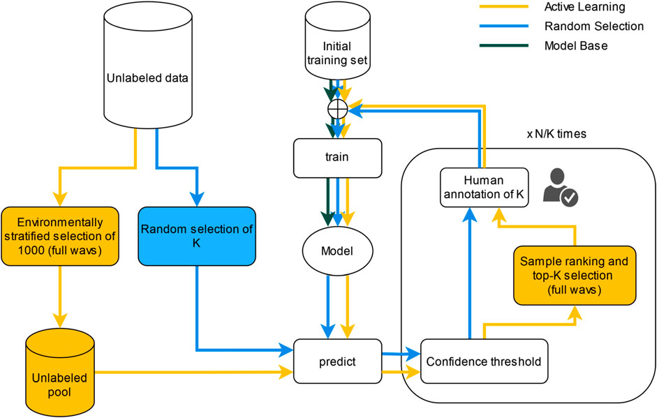
Figure 4. Flows of the three different compared approaches of the Object detector model to add more data. The Model Base is the model obtained on iteration number 0 on any of the two flow charts (training only on the initial training set).

Annotating boxes is time-consuming, and using pre-annotated boxes has been found to increase annotation speed and improve model performance on other object detection tasks (Fennell et al., 2022). Hence we used a model-assisted annotation strategy to revise and correct predictions instead of manually adding all the sound events from scratch. Even though from a machine learning perspective it would be more efficient to select individual 20-s snippets from different files rather than full wav files, this is not a common practice for bioacousticians. The process to select more files for each approach is explained in the following sections.

2.6.1 Random sampling

For the random sampling approach, 10 wav files were randomly selected from all the available files, that were not part of the training or test sets. These files were converted into images as explained in Section 2.4. The images were then predicted using the Model Base and the output was transformed to a Raven-compatible format as explained in 2.5.2. The output of the Model Base was used as initial predictions for model-assisted annotation. The 10 randomly selected files were manually revised and corrected using Raven. Then the 10 selected files were randomly split into 5 groups of 2 to simulate the incremental addition of data. This process was repeated 3 times, one per each Model Base.

2.6.2 Active learning

For the active learning approach, the files to be annotated from the unlabeled pool were determined by the model. This was done by choosing the 2 files scoring the highest following a criteria decided with 3 objectives:

• Find new and rare sounds compared to the training set

• Reduce the uncertainty of the model (i.e., providing more training examples of sounds with high prediction uncertainty)

• Chose a file with a high diversity of sounds

To find rare and new sounds, for each detection in the unlabeled pool we computed the 90th percentile of spectro-temporal overlap with all the detections within the previous training set, as specified in Eqs (1) and (2). If this value is low, it implies that the overlap with most of the current training dataset is low, and therefore it is a sound event in a new frequency band or a different duration, which is a proxy for the novelty of the sound.

${\mathrm{i}\mathrm{o}\mathrm{u}}_{ij}=\frac{\left(\min \left(f_{\text{high},i},f_{\text{high\hspace{0.17em}},j}\right)-\max \left(f_{\text{low},i},f_{\text{low},j}\right)\right)\min \left(w_i,w_j\right)}{A_i}(1)$

${\mathrm{i}\mathrm{o}\mathrm{u}}_i=\left[{\mathrm{i}\mathrm{o}\mathrm{u}}_{i,0},{\mathrm{i}\mathrm{o}\mathrm{u}}_{i,1},\dots ,{\mathrm{i}\mathrm{o}\mathrm{u}}_{i,n}\right];{\mathrm{i}\mathrm{o}\mathrm{u}}_{i,\mathrm{90}\mathrm{t}\mathrm{h}}={\mathrm{i}\mathrm{o}\mathrm{u}}_i\left(\lceil 0.9n\rceil \right)(2)$

where,

f_high,i is the upper frequency limit of the detection i,

f_low,i is the lower frequency limit of the detection i,

w_i is the duration of the detection i,

A_i = (f_high,i − f_low,i)w_i is the area of the detection i,iou_ij is the intersection over union between detection i and j,

n is the number of detections in the training set.

We defined the uncertainty of each detection as u_i = 1 − c_i, where c_i is the confidence of the detection i. The number of ‘interesting’ sounds in a wav file was then computed considering an uncertainty threshold of 0.75 and an overlap threshold of the 90th percentile, as specified in Eq. (3).

$N_{\text{wav}}={\displaystyle \sum _{i=0}^m}\left[u_i>0.75\text{\hspace{0.17em}and\hspace{0.17em}}{\mathrm{i}\mathrm{o}\mathrm{u}}_i<{\mathrm{i}\mathrm{o}\mathrm{u}}_{90\text{th}}\right](3)$

where,

iou_90th is the 90th percentile considering all the iou_i,90th.

Finally, we computed the diversity of sounds within a file by computing the entropy of the overlapping matrix of all the detections of one wav file (O_wav in Eq. (4)), as specified in Eqs (5) and (6).

$O_{\text{wav}}=\left[\begin{array}{cccc}\hfill d_{\mathrm{0,0}}\hfill & \hfill d_{\mathrm{0,1}}\hfill & \hfill \dots \hfill & \hfill d_{\mathrm{0,100}}\hfill \\ \hfill \dots \hfill & \hfill \dots \hfill & \hfill \dots \hfill & \hfill \dots \hfill \\ \hfill \dots \hfill & \hfill \dots \hfill & \hfill d_{k,l}\hfill & \hfill \dots \hfill \\ \hfill d_{\mathit{100,0}}\hfill & \hfill \dots \hfill & \hfill \dots \hfill & \hfill d_{\mathit{100,100}}\hfill \end{array}\right](4)$

$d_{k,l}={\displaystyle \sum _{i=0}^m}\frac{\left[f_{\text{low},i}>\frac{f_{\text{nyq}}}{k}>f_{\text{high},i}\text{\hspace{0.17em}and\hspace{0.17em}}{w}_i>\frac{D_{\text{max}}}{l}\right]}{m}(5)$

$E_{\text{wav}}={\displaystyle \sum _{\begin{array}{c}k,l\end{array}}}{d}_{k,l}\ln \left(d_{k,l}\right)\text{\hspace{0.17em}if\hspace{0.17em}}{d}_{k,l}\ne 0(6)$

where,

O_wav is the overlap matrix of one wav file with the training set,

d_k,l is the overlap computed at frequency index k and time index l,

f_nyq is half the sampling frequency (12,000 Hz),

D_max is the maximum duration of all the detections in the unlabeled pool,

m is the number of detections within the wav file,

E_wav is the entropy of the wav file.

Finally, a third component was added to the score to allow the selection of a file based on the presence of one unique sound. We decided to give more weight to adding unseen sounds to the training set as the acoustic richness is reflected by these rare sounds. A rare sound with a very low overlap with the training set and a low confidence in detection, as it should be a shape never seen by the model.

Therefore, the final score of each wav was computed as shown in Eq. (7):

$s_{\mathrm{w}\mathrm{a}\mathrm{v}}=\frac{N_{\text{wav}}}{d_{\text{wav}}}\max \left(\left(1-{\mathrm{i}\mathrm{o}\mathrm{u}}_i\right)u_i\forall i\in \mathrm{w}\mathrm{a}\mathrm{v}\right)E_{\text{wav}}(7)$

where,

d_wav is the duration of the file in seconds,

s_wav is the score of the wav file.

The overall wav scores were used to select the two files with the highest score at every loop iteration. After 2 iterations, a 30% probability was set of replacing one of the selected files with a randomly selected one. This was done to consider the possibility that not all factors influencing acoustic diversity within the data were considered with this approach, and to not bias the model towards learning on only acoustically divers files.

The selection of files was done in 5 loop iterations; 2 files were selected each time for annotation, and subsequently removed from the pool of unlabeled data. At each loop iteration, the annotation was carried out using the model-assisted annotation strategy, always using the model obtained at the previous loop iteration for prediction.

2.7 Clustering and continuous data analysis

To prove the applicability of the method we applied it in one short deployment from the LifeWatch Broadband Acoustic Network, the deployment from the Grafton station starting the 27th of October of 2022. This deployment consists of a 10 days of recordings with a duty cycle of 50% (1 day on, 1 day off) at a fixed location at the Grafton station. This is intended as a show case to prove the usability of the proposed methodology, and to illustrate how this pipeline can be used for soundscape characterization.

The deployment’s audio data were converted to the YOLOv8 format as explained in Section 2.4, and the final model was used to extract a collection of possible sounds events (detections) for subsequent clustering on the 20-s images. The predictions were joined as explained in Section 2.5.2. A minimum confidence of 0.1 was chosen for predictions being considered as sound event detections.

Using the start and end times of the obtained detections, raw audio snippets were obtained for each detection and converted into a embedding feature space using the pre-trained BioLingual model (Robinson et al., 2023), which is a state-of-the-art model for latent representation for classification of bioacoustics signals across multiple datasets. This model extracts 512 deep embedding acoustic features. The maximum length for a snippet was set to 2 s with shorter detections being zero-padded, while longer detections being cut to 2 s. Each detection was filtered with a bandpass filter of order 4 to the band of interest of the detected event (between its minimum and maximum frequency).

The BPNS dataset presents a high imbalance between broadband, short, impulsive sounds and other longer, more complex sounds. To avoid obtaining only one big cluster with these events and another one with the rest, all the detections shorter than 0.3 s were classified as impulsive sounds and excluded from the clustering. Such short sounds, even though they can be ecologically relevant, are often not classified by their waveform but according to their frequency limits or peak. Therefore acoustic features extracted by the BioLingual model were not expected to provide enough information on further cluster separation for these types of sounds.

For the rest of the detections, the extracted BioLingual features were reduced to a 2D space using UMAP (McInnes et al., 2020) with the number of neighbors set to 10 and a minimum distance set to 0.2. The UMAP dimension reduction was applied to deal with the high-dimensional data resulting from extracting the BioLingual features (512 features), as done previously in Phillips et al. (2018) and Best et al. (2023). This problem is known as the “curse of dimensionality”, and density based clustering algorithms such as HDBSCAN are known to provide low performance in high dimensional spaces. Then the python implementation of HDBSCAN (McInnes et al., 2017) was applied to the resulting 2D embedding space, and the minimum number of samples (events, in this case) per cluster was set to 5 to allow for rare sounds to form a cluster. The epsilon to select the clusters was set to 0.05, and the minimum number of neighbors to 150. All the parameters were selected to get a balance between noise removal and robustness of clusters.

All the obtained clusters were manually revised for possible significance by manually checking a minimum of 10 randomly selected events per cluster. If more than 7 of the revised events were clearly similar sounds, the cluster was assigned a possible source category if previous knowledge was available. The possible categories included pseudo-noise, geophonic, mooring noise, instrument noise, anthropogenic sounds, and biological. When none of these categories could be assigned with certainty, clusters were labeled as unknown. If less than 7 of the revised events per cluster were clearly similar sounds, the cluster was labeled as unclear.

Once all the obtained detections were assigned to a cluster, the different clusters’ occurrences were plotted in time to check for diel patterns, adding the sunset and sunrise timestamps to check for dusk/dawn patterns. Furthermore, the temporal patterns were assessed and compared among clusters. This was done by plotting the average percentage of positive detection minutes (minutes where there was at least one detection of that cluster) for each 15 min bin.

3 Results

3.1 Detection results

Several models were trained and their performances were compared on the independent test sets: 3 Model Base (MB) using the initial training set, 15 models with incremental training data using random selection (RS), and 15 models with incremental training data using active learning (AL) selection. Additionally to the model evaluation on the separate BPNS test dataset, obtained models were also evaluated on the freshwater test set to test their robustness to new data. We also trained a model using all the available annotated data from the BPNS (initial training set, added annotations from both the random and active learning selection approaches, and test set), and evaluated its performance on the freshwater dataset. We will refer to this model as Model Final (MF) from now on.

Regarding the strategy of adding files, the active learning approach presented a faster improvement curve than the random sampling. For the BPNS test set, recall stayed constant for both approaches and did not improve. For the freshwater dataset, precision of the two approaches presented similar values (see Figure 5). The performance of the active learning approach converged at the end of file addition, due to the fact that the three repetitions ended up selecting some of the same files. When comparing the average performances of the models from the last training iteration (for active learning, AL5, for random sampling RS5) and the Model Base (MB)on the BPNS test set, AL5 outperformed RS5 and Model Base on 6 metrics, and led to the best F1 score of 56.69% (see Table 2).

Figure 5

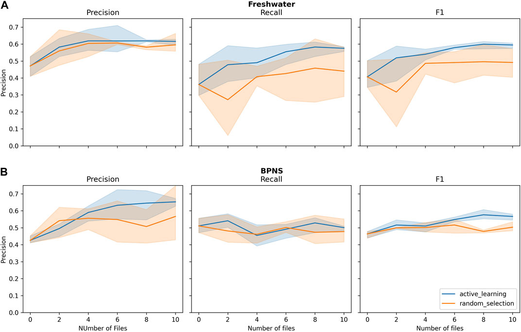
Figure 5. Evaluation metrics on (A) freshwater test set and (B) BPNS test set. X-axis represents the number of additional annotated files using the active learning (AL) and random selection (RS) method for selecting these files. Shaded area represents the minimum and maximum, and the line represents the mean value.

Table 2

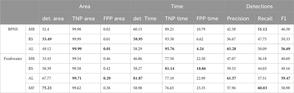
Table 2. Average performance of the final models. MB stands for Model Base, AL for Active Learning, RS for Random Sampling and MF for Model Final in percentage. Area metrics are the ones computed considering both frequency and time. Time metrics are the ones considering only times. det area/time stands for percentage of detected area/time, TNP stands for True Negative Percentage, and FPP stands for False Positive Percentage. Detection metrics are computed by counting overlapping boxes, with a iou threshold set to 0.1 to compute precision, recall and F1. Best result per metric and test set is marked in bold. All results are including predictions with a confidence of 0.1 or more. The minimum and maximum values of MB, RS and AL can be seen as the first and last points of the evolution curves on Figure 5.

When evaluating models MB, AL5, RS5 and MF on the freshwater test set, the performance is comparable to the metrics obtained in the BPNS test set (see Table 2). This proves that the model is robust across datasets and can be used on data from unseen locations. For the freshwater test set, AL5 also outperformed RS5 approach in all the metrics except TNP and FPP (time). It also outperformed MF in several metrics including precision and F1.

The detected percentage for both area and time in the freshwater test set is better than in the BPNS set, but worse when looking TNP and FPP (both time and area). This points out differences between the events distribution in time and frequency between the two test sets. Within each test set, TNP and FPP are best when computed for area, while detection percentage is best when computed for time.

3.2 Clustering and continuous data analysis

The final model detected a total of 197,793 events during the 10 days of the deployment (6 days of data, a total of 705 wav files). From all the obtained (joined) detections, 90.91% were detections shorter than 0.3 s. These were not converted to the embedding space and were classified as impulsive sounds.

For the rest of the detections, the UMAP 2D space applied to the BioLingual embedded feature space presented a clear cluster structure (see Figure 6). When applying HDBSCAN to the 2D space, 8 clusters were obtained (see Figure 6). All the clusters were manually revised as explained in Section 2.7, and assigned a label and a possible source. The output of these revision is listed in the Supplementary Material Supplementary Table S2, where textual descriptions, mean frequency limits and duration information (10th and 90th percentile) are provided for each cluster.

Figure 6

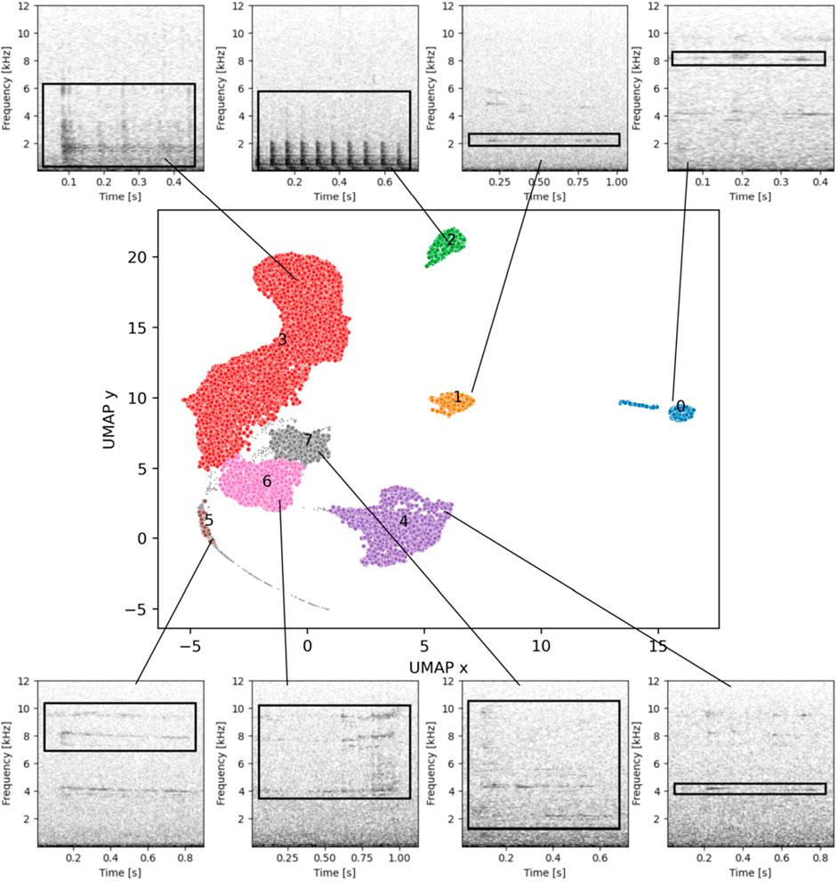
Figure 6. The UMAP 2D reduction colored by obtained clusters and one spectrogram example for each cluster. For the spectrogram generation, the number of FFT bins was 512, with an overlapping of 480 samples, Hann window. A black box has been added to show the frequency limits of each detection.

The clusters were then grouped by source type, and the number of clusters and percentages of each source type were summarized (see Table 3). From the 9.09% selected for further clustering, the biological/pseudo-noise were the group with most detections (52.26%), followed by unknown (non-impulsive) sources (42.06%), and finally biological (3.11%).

Table 3

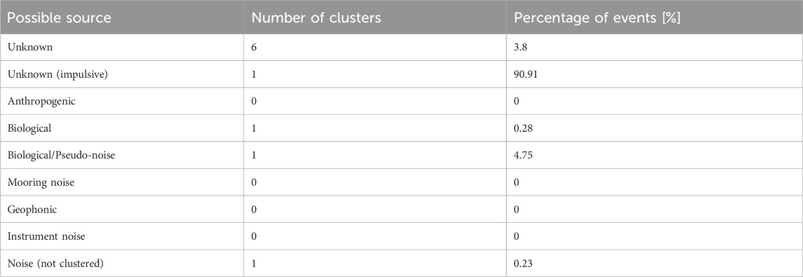
Table 3. Summary of the classification of all the obtained clusters.

From all the obtained clusters, only one could be identified as biological with certainty (cluster 2). This cluster was formed by sound events with a high repetition rate, and a frequency spanning from around 100 to 4,000 Hz (see Supplementary Table S2 from Supplementary Material). We refer to it as “Jackhammer”. The number of pulses was not constant at each detected event, ranging from 2 to 70 pulses, but with a majority of them around 10–15 pulses. The repetition rate was around 14 pulses/second. When analyzing 15-minute occurrence of this cluster in time (see Figure 7), the number of detections seem to be higher at dawn. However, these sound events were mostly detected only on two different days, within a specific time frame lasting between 2 and 5 h, while absent the rest of the days.

Figure 7

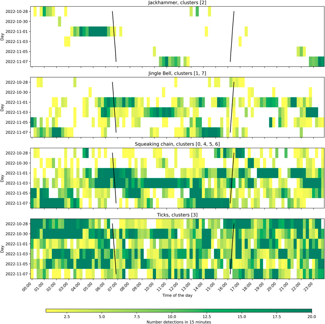
Figure 7. Daily patterns of the number of detections of the selected classes every 15 min. Black lines represent sunset and sunrise.

Two “metallic” sounds were found throughout the analyzed recordings, classified in 6 different clusters due to its variability. From these clusters, two main groups could be extracted, with clusters 6 and 7 being the representation for each group, respectively. Group represented by cluster 7 was defined as a clear jingle-bell-like sound at different frequencies, from 1.5 to 8 kHz, with usually several harmonics and a duration of around 1 s. Cluster 1 was a single harmonic from this sound, sometimes selected within the full sound, and sometimes found alone probably because of propagation loss. The sound represented by cluster 1 and 7 was named “Jingle bell”. On the other hand, group represented by cluster 6 was labeled sounding as a “squeaking chain” and it was present at higher frequencies, from 4 to 10 kHz. It often looks like a down sweep, and it has no impulsive component at the beginning. When complete (cluster 6), it also presents harmonics and also a duration of around 1 s. Clusters 0, 4, and 5 were labeled as harmonics from this sound, also sometimes selected within the full sound. This group was labeled as “Squeaking chain.”

Cluster 3 was repetition of impulsive sounds, sounding like a wooden scratch. It presented simultaneously a semi-constant tonal component at around 2 kHz and several impulsive sounds. These impulsive sounds were present both broadband or very narrow band. We named it “Ticks.”

When analyzing the temporal distribution of the clusters, no clear patterns could be seen. The polar plot in Figure 8 revealed that the “jackhammer” happened mostly at dawn. “Jingle bell” and “squeaking chain” seemed to have similar patterns, with a slight increase during the day. “Ticks” presented a higher density during the night than during the day, but there were also detections during the day.

Figure 8

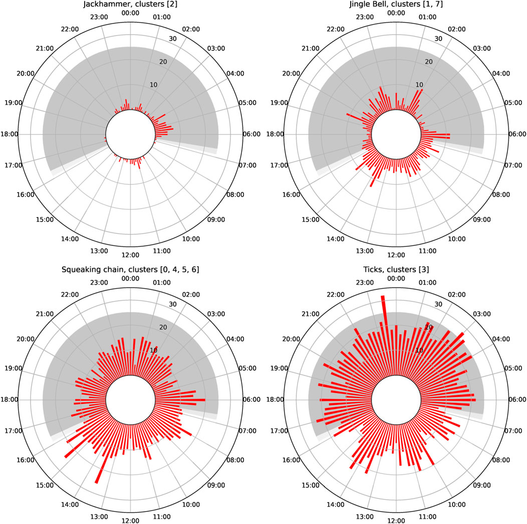
Figure 8. Polar plot of the detection distribution per class depending on the hour of the day for the Grafton deployment. Radius represents the percentage of minutes where at least one detection was present in the corresponding 15 min bin.

4 Discussion

In this study we show a novel methodology to analyze underwater soundscapes in areas where very few sound sources have been previously described. The method helps to gain insight into the different (recurrent) sound sources in the soundscape, and allows for an automatic detection and categorization of sound events with limited human effort. With this methodology, soundscape analysis could provide meaningful insight even though the sources of the different sound types are not known.

The performance achieved by the object detector model on the test set using any of the three models (base model, random sampling, and active learning) was comparable to human performance. This is especially true in data scenarios where annotation is challenging, such as when high ambient noise levels mask the sound events of interest (Leroy et al., 2018; Nguyen Hong Duc et al., 2021). Not knowing which are the sound events of interest adds an extra challenge and inconsistency. The concept of acoustical and visual saliency is subjective. Differentiating foreground events from background noise depends on the human analyst and the selected settings and goals during annotation, as there is no clear separation between foreground and background but rather a continuum of levels of masking. An example of this challenge is shown in Supplementary Figure S1 of Supplementary Material, where model predictions and human annotations are diverging substantially, but the ground truth annotations are very subjective.

The overall obtained F1 values were not high, but TNP and FPP presented an overall good performance, both when looking at the area and the time metrics. This is partly due to the sparseness of the sound events, which makes TNP and FPP suited metrics to evaluate the performance in long-term data. Furthermore, the performance of the detection model was proven to be robust across locations and ecosystems, as it performed better in data from a location that was not used for any training, even from a complete different ecosystem such as freshwater. The fact that the obtained models (AL5, RS5 and MF) performed overall better in the freshwater test set than in the BPNS test set might be because the freshwater recordings are less noisy than those of the BPNS, which is known to be an extremely noisy environment (Parcerisas et al., 2023). However, even though the models performed better in the freshwater test set than in the BPNS regarding recall, F1 and detected percentage (area and time), they performed worse when looking at TNP and FPP. This could be due to differences regarding quantity, simultaneity and segmentation of events between the two test sets.

The active learning approach led to better results overall than the random sampling approach. The files selected for active learning presented a higher acoustic complexity than the ones selected randomly. This supports the hypothesis that the metric used to select wav files points to more complex files. The model overall performs better (considering all metrics) when complex files are selected because it can learn how to solve complex situations in a more similar manner to a human annotator. However, the more complex the sounds, the higher is the challenge for the model to find all different sound events (hence the reduction in recall). It is necessary to note that the files selected by the active learning algorithm presenting a higher acoustic diversity might not necessarily represent higher biophonic activity. Furthermore, the files selected by the algorithm are based on the detections from the previous model, which means that totally new sounds could be completely missed (as they are not detected by the model at all). The active learning selection method thus does not assure the addition of unseen new and interesting sounds, but it has been proven to be more effective than the random selection of files. Therefore, if a model has to be re-trained and the available annotation time is limited, the active learning approach can deliver better results while investing less time on annotations. These findings are in line with other studies applying active learning to detect sounds on long-term recordings to extract ecological information (Kholghi et al., 2018; Hilasaca et al., 2021), pointing out that active learning is an interesting field to explore when human annotations from long-term recordings are necessary to train machine learning models.

The trained detection model can be applied to data from other locations, as it has been proven with the freshwater dataset. The model as it is, provides a performance similar to the human performance, so it can be used right away on other ecosystems. Yet, it might miss some sounds of interest, especially if applied on a different frequency range. A good approach for future fine tuning or re-training of this model would be to first create a base model trained with a balanced annotated dataset containing interesting sounds and a variety of environmental conditions. This way the model can learn from the beginning a good variety of shapes on the spectrogram.

In this study we prove that the BioLingual (Robinson et al., 2023) model together with a UMAP 2D (McInnes et al., 2020) reduction provided enough information to obtain clear and meaningful clusters. The manual revision of the obtained clusters indeed led to the conclusion that the clusters were acoustically meaningful and represented different sound types. Therefore it can be concluded that the BioLingual features contained enough information, and that the reduction to a 2D dimension using UMAP maintained the general density structure. The combination of UMAP reduction on a feature space together with HDBSCAN (McInnes et al., 2017) algorithm applied on the reduced dimension was already successfully applied by Sainburg et al. (2020), Thomas et al. (2022) and Best et al. (2023) to separate different biological sound events, so our results align with their proposal. However, in all these approaches the sound events were manually selected. The novelty of our proposed approach is that the whole process is automatized.

Regarding the application of the clustering to data from other environments, a new clustering algorithm on a new deployment would provide a different set of clusters, not necessarily comparable with the clusters obtained from previously analyzed deployments. To compare soundscapes between different deployments in the same regions, it is sometimes interesting to keep the existing clusters in order to track the changes in sound events. This should be possible if a large and representative enough dataset of detections is first clustered. Then it is possible to query the HDBSCAN model on small amounts of new data (McInnes et al., 2017). The python implementation of HDBSCAN allows for this, by holding a clustering fixed and then find out where in the condensed tree the new data would fall. The first representative dataset to cluster events can be manually annotated or can also be the outcome of the detection model ran on a selected set of files representing all the possible ecological conditions of interest, and multiple instances of all the expected sound types.

On the presented study we focused on a broadband frequency range, from 0 to 12 kHz. This decision was made so some cetacean sounds would also be included without risking not seeing low frequency sounds in the spectrogram. In the particular case of this study we focused on the entire frequency band equally. This means that when manually annotating a broadband frequency range, very narrow-band sounds can be easily missed, especially the ones in the lower frequency range. As expected then, the model might also miss these sounds as it has not been trained on those. Nonetheless, the same method could be applied to smaller frequency ranges, for example from 0 to 3 kHz if the interest would be focused on fish vocalizations (Amorim, 2006). The model should work regardless of the frequency range as long as the time and frequency resolution are enough to represent the sounds of interest. In future work it would be interesting to train the model with a logarithmic frequency scale to emphasize lower frequency sounds and compare the performance of both models.

In this particular case, due to the abundance of very short impulsive sounds ($<$ 0.3 s), a first separation among detections was applied. This should not be necessary in areas where there is not one sound type dominating and generating this high imbalance, or where impulsive sounds (clicks) are not present. Because of the lack of knowledge and information regarding this impulsive sounds, we just cluster them according to their frequency limits. This is in line with the thesis by Harland (2017), where clicks (impulsive sounds) heard in the UK waters were characterized and identified. Future research would be needed to assess the source of this impulsive sounds and their ecological significance, but nothing discards them coming from biological sources Kim et al. (2009); Coquereau et al. (2016); Cole (2010). If the analyzed location contains click sequences and the model was not trained to recognize them as sequences but just as individual pulse units, they would not appear as a sequence cluster. However, a posterior analysis from all the impulsive sounds complying with the frequency limits of interest could be analyzed for temporal patterns and join the clicks into sequences.

When analyzing the obtained clusters in the deployment, the obtained sound types are similar to the ones mentioned in Calonge et al. (2024), who did a clustering analysis from labeled manual annotations. This points out the robustness of the model, and highlights the reduction of manual input to reach similar conclusions. Only one sound was found fitting within the known description of fish sounds, as it is within the known vocalization frequency range of fish, and it is a repetitive set of impulse sounds (Amorim, 2006; Carriço et al., 2019). There have been similar fish sounds reported in literature from the family Sciaenidae (Amorim et al., 2023), and an invasive species of this family has been documented in the North Sea (Morais et al., 2017). However, these assumptions have to be taken with the most caution as ground truth has not been confirmed. The obtained cluster “Ticks” could maybe come either from bio-abrasion of the hydrophone (Ryan et al., 2021), invertebrates or fish clicking sounds (Harland, 2017). Finally two different metallic sounds were found. These could originate from the mooring itself, as it is a steel mounting system (even though it has no moving parts), but could also be related to invertebrate sounds, such as the ones mentioned in Coquereau et al. (2016). The fact that these two sounds appeared in multiple clusters is because the sound did not present all the harmonics all the time, probably due to propagation loss (Forrest, 1994) or sound production inconsistency. With the presented approach, bounding boxes from sound events can overlap as long as iou is less than 0.5, otherwise they are joined and considered the same detection. Therefore, harmonic sounds can potentially be selected in multiple boxes at the same time. This is advantageous because when these harmonics appear by themselves they are clustered together with the boxes that overlap with the full sound, so they can be traced back to their origin. However it can be disadvantageous because it can complicate the counting of sound occurrences.

The shown case study provides an example of the analysis that can be performed with the outcome of the presented model pipeline. This analysis can provide insight on the spatio-temporal patterns of certain sound types, which in the long term can be used to discover their source. With this methodology it is possible to already obtain ecological information at the same time that researchers discover the sources of sounds and gain insight on the soundscape. However, once a sound source is identified, considered of interest, and adequately characterized, other supervised techniques might be more efficient and provide a greater performance for sound event detection and posterior soundscape analysis and description (Stowell, 2022; Barroso et al., 2023). For this reason it is necessary to create databases of sounds where well-described unidentified sounds can also be added, so in the future they can be used as references (Parsons et al., 2022).

In conclusion, the proposed method is a useful tool to discover unknown sounds in a new environment and can be used as a first analysis tool. Implementing this methodology in already available annotation or exploration software such as PAMGuard (Gillespie et al., 2009), Whombat (Balvanera et al., 2023) or RavenPro (K. Lisa Yang Center for Conservation Bioacoustics at the Cornell Lab of Ornithology, 2023) can help addressing some of the challenges encountered when studying underwater soundscapes with little known sound sources. The obtained model is robust to different environments and can be applied directly to new data, even though for higher performance it would be recommended to re-train on a subset of this new data. The principal advantage of this model is that it is not based on previous assumptions of which sounds could be of interest, as all the possible events are detected and classified. Furthermore, it provides a framework for discovering the sound types while already gaining ecological insight of the soundscape. The proposed methodology helps in filling the gap in knowledge on sound types, which is currently major issue for using PAM for ecological assessment of the underwater environment (Rountree et al., 2019; Mooney et al., 2020; Parsons et al., 2022).

Data availability statement

The full dataset from the BPNS can be found on IMIS (https://marineinfo.org/id/dataset/78799), and is open and available upon request. The recordings selected from the full BPNS dataset and used for training and evaluating the model are available in MDA (https://doi.org/10.14284/667). The code used for the analysis of this paper can be found on github (https://github.com/lifewatch/sound-segregation641 and-categorization).

Author contributions

CP: Conceptualization, Data curation, Formal Analysis, Methodology, Software, Visualization, Writing–original draft, Writing–review and editing. ES: Conceptualization, Supervision, Writing–review and editing. KV: Validation, Writing–review and editing. DB: Supervision, Writing–review and editing. PD: Supervision, Writing–review and editing. ED: Funding acquisition, Project administration, Resources, Supervision, Writing–review and editing.

Funding

The author(s) declare that financial support was received for the research, authorship, and/or publication of this article. This research was funded by LifeWatch grant number I002021N. ES’s contribution to this research was funded by FWO grant number V509723N.

Acknowledgments

The project was realized as part of the Flemish contribution to LifeWatch. The authors thank the Simon Stevin RV crew for their help with the deployment and retrieval of the acoustic instruments. We would like to thank the maps team at VLIZ for the location map. The authors want to thank Julia Aubach, Svenja Wohle, Quentin Hamard, Zoe Rommelaere, Coline Bedoret, Kseniya Mulhern and Olayemi Saliu who helped with the annotation of the data.

Conflict of interest

The authors declare that the research was conducted in the absence of any commercial or financial relationships that could be construed as a potential conflict of interest.

Publisher’s note

All claims expressed in this article are solely those of the authors and do not necessarily represent those of their affiliated organizations, or those of the publisher, the editors and the reviewers. Any product that may be evaluated in this article, or claim that may be made by its manufacturer, is not guaranteed or endorsed by the publisher.

Supplementary material

The Supplementary Material for this article can be found online at: https://www.frontiersin.org/articles/10.3389/frsen.2024.1390687/full#supplementary-material

References

Amorim, M. C. (2006). Diversity of sound production in fish. Commun. Fishes 1, 71–105.

Google Scholar

Amorim, M. C. P., Wanjala, J. A., Vieira, M., Bolgan, M., Connaughton, M. A., Pereira, B. P., et al. (2023). Detection of invasive fish species with passive acoustics: discriminating between native and non-indigenous sciaenids. Mar. Environ. Res. 188, 106017. doi:10.1016/j.marenvres.2023.106017

PubMed Abstract | CrossRef Full Text | Google Scholar

Au, W. W. L., and Hastings, M. C. (2008). Principles of marine bioacoustics. New York, NY: Springer US. doi:10.1007/978-0-387-78365-9

CrossRef Full Text | Google Scholar

Bagherinezhad, H., Horton, M., Rastegari, M., and Farhadi, A. (2018). Label refinery: improving ImageNet classification through label progression. doi:10.48550/arXiv.1805.02641

CrossRef Full Text | Google Scholar

Balvanera, S. M., Mac Aodha, O., Weldy, M. J., Pringle, H., Browning, E., and Jones, K. E. (2023). Whombat: an open-source annotation tool for machine learning development in bioacoustics. doi:10.48550/arXiv.2308.12688

CrossRef Full Text | Google Scholar

Barroso, V. R., Xavier, F. C., and Ferreira, C. E. L. (2023). Applications of machine learning to identify and characterize the sounds produced by fish. ICES J. Mar. Sci. 80, 1854–1867. doi:10.1093/icesjms/fsad126

CrossRef Full Text | Google Scholar

Best, P., Paris, S., Glotin, H., and Marxer, R. (2023). Deep audio embeddings for vocalisation clustering. PLOS ONE 18, e0283396. doi:10.1371/journal.pone.0283396

PubMed Abstract | CrossRef Full Text | Google Scholar

Bolgan, M., Gervaise, C., Di Iorio, L., Lossent, J., Lejeune, P., Raick, X., et al. (2020). Fish biophony in a Mediterranean submarine canyon. J. Acoust. Soc. Am. 147, 2466–2477. doi:10.1121/10.0001101

PubMed Abstract | CrossRef Full Text | Google Scholar

Calonge, A., Parcerisas, C., Schall, E., and Debusschere, E. (2024). Revised clusters of annotated unknown sounds in the Belgian part of the North Sea. Front. Remote Sens.

Google Scholar

Carriço, R., Silva, M. A., Menezes, G. M., Fonseca, P. J., and Amorim, M. C. P. (2019). Characterization of the acoustic community of vocal fishes in the Azores. PeerJ 7, e7772. doi:10.7717/peerj.7772

PubMed Abstract | CrossRef Full Text | Google Scholar

Cole. K. S. (2010). Reproduction and sexuality in marine fishes: patterns and processes (Berkeley: Univ. of California Press).

Google Scholar

Coquereau, L., Grall, J., Chauvaud, L., Gervaise, C., Clavier, J., Jolivet, A., et al. (2016). Sound production and associated behaviours of benthic invertebrates from a coastal habitat in the north-east Atlantic. Mar. Biol. 163, 127. doi:10.1007/s00227-016-2902-2

CrossRef Full Text | Google Scholar

Desiderà, E., Guidetti, P., Panzalis, P., Navone, A., Valentini-Poirrier, C.-A., Boissery, P., et al. (2019). Acoustic fish communities: sound diversity of rocky habitats reflects fish species diversity. Mar. Ecol. Prog. Ser. 608, 183–197. doi:10.3354/meps12812

CrossRef Full Text | Google Scholar

Di Iorio, L., Audax, M., Deter, J., Holon, F., Lossent, J., Gervaise, C., et al. (2021). Biogeography of acoustic biodiversity of NW Mediterranean coralligenous reefs. Sci. Rep. 11, 16991. doi:10.1038/s41598-021-96378-5

PubMed Abstract | CrossRef Full Text | Google Scholar

EMODnet Bathymetry Consortium (2018). EMODnet digital Bathymetry (DTM 2018). doi:10.12770/bb6a87dd-e579-4036-abe1-e649cea9881a

CrossRef Full Text | Google Scholar

Fennell, M., Beirne, C., and Burton, A. C. (2022). Use of object detection in camera trap image identification: assessing a method to rapidly and accurately classify human and animal detections for research and application in recreation ecology. Glob. Ecol. Conservation 35, e02104. doi:10.1016/j.gecco.2022.e02104

CrossRef Full Text | Google Scholar

Forrest, T. G. (1994). From sender to receiver: propagation and environmental effects on acoustic signals. Am. Zool. 34, 644–654. doi:10.1093/icb/34.6.644

CrossRef Full Text | Google Scholar

GEBCO Compilation Group (2022). GEBCO_2022 grid. doi:10.5285/e0f0bb80-ab44-2739-e053-6c86abc0289c

CrossRef Full Text | Google Scholar

Gillespie, D., Mellinger, D. K., Gordon, J., McLaren, D., Redmond, P., McHugh, R., et al. (2009). PAMGUARD: semiautomated, open source software for real-time acoustic detection and localization of cetaceans. J. Acoust. Soc. Am. 125, 2547. doi:10.1121/1.4808713

CrossRef Full Text | Google Scholar

Harland, E. J. (2017). An investigation of underwater click sounds of biological origin in UK shallow waters. Ph.D. thesis. Southampton, United kingdom: University of Southampton.

Google Scholar

Havlik, M.-N., Predragovic, M., and Duarte, C. M. (2022). State of play in marine soundscape assessments. Front. Mar. Sci. 9. doi:10.3389/fmars.2022.919418

CrossRef Full Text | Google Scholar

Hilasaca, L. H., Ribeiro, M. C., and Minghim, R. (2021). Visual active learning for labeling: a case for soundscape ecology data. Information 12, 265. doi:10.3390/info12070265

CrossRef Full Text | Google Scholar

Jocher, G., Chaurasia, A., and Qiu, J. (2023). YOLO by ultralytics.

Google Scholar

Kholghi, M., Phillips, Y., Towsey, M., Sitbon, L., and Roe, P. (2018). Active learning for classifying long-duration audio recordings of the environment. Methods Ecol. Evol. 9, 1948–1958. doi:10.1111/2041-210X.13042

CrossRef Full Text | Google Scholar

Kim, B.-N., Hahn, J., Choi, B., and Kim, B.-C. (2009). Acoustic characteristics of pure snapping shrimp noise measured under laboratory conditions.

Google Scholar

K. Lisa Yang Center for Conservation Bioacoustics at the Cornell Lab of Ornithology (2023). Raven Pro: interactive sound analysis software. Ithaca, NY, Unites States: The Cornell Lab of Ornithology. Version 1.6.4.

Google Scholar

Lamont, T. A. C., Chapuis, L., Williams, B., Dines, S., Gridley, T., Frainer, G., et al. (2022). HydroMoth: testing a prototype low-cost acoustic recorder for aquatic environments. Remote Sens. Ecol. Conservation 8, 362–378. doi:10.1002/rse2.249

CrossRef Full Text | Google Scholar

Leroy, E. C., Thomisch, K., Royer, J.-Y., Boebel, O., and Van Opzeeland, I. (2018). On the reliability of acoustic annotations and automatic detections of Antarctic blue whale calls under different acoustic conditions. J. Acoust. Soc. Am. 144, 740–754. doi:10.1121/1.5049803

PubMed Abstract | CrossRef Full Text | Google Scholar

Lin, T.-Y., Maire, M., Belongie, S., Bourdev, L., Girshick, R., Hays, J., et al. (2015). Microsoft COCO: common objects in context. doi:10.48550/arXiv.1405.0312

CrossRef Full Text | Google Scholar

Looby, A., Cox, K., Bravo, S., Rountree, R., Juanes, F., Reynolds, L. K., et al. (2022). A quantitative inventory of global soniferous fish diversity. Rev. Fish. Biol. Fish. 32, 581–595. doi:10.1007/s11160-022-09702-1

CrossRef Full Text | Google Scholar

McInnes, L., Healy, J., and Astels, S. (2017). Hdbscan: hierarchical density based clustering. J. Open Source Softw. 2, 205. doi:10.21105/joss.00205

CrossRef Full Text | Google Scholar

McInnes, L., Healy, J., and Melville, J. (2020). UMAP: uniform manifold approximation and projection for dimension reduction. doi:10.48550/arXiv.1802.03426

CrossRef Full Text | Google Scholar

Minier, L., Bertucci, F., Raick, X., Gairin, E., Bischoff, H., Waqalevu, V., et al. (2023). Characterization of the different sound sources within the soundscape of coastline reef habitats (Bora Bora, French Polynesia). Estuar. Coast. Shelf Sci. 294, 108551. doi:10.1016/j.ecss.2023.108551

CrossRef Full Text | Google Scholar

Mooney, T. A., Di Iorio, L., Lammers, M., Lin, T.-H., Nedelec, S. L., Parsons, M., et al. (2020). Listening forward: approaching marine biodiversity assessments using acoustic methods. R. Soc. Open Sci. 7, 201287. doi:10.1098/rsos.201287

PubMed Abstract | CrossRef Full Text | Google Scholar

Morais, P., Cerveira, I., and Teodósio, M. A. (2017). An update on the invasion of weakfish cynoscion regalis (bloch and schneider, 1801) (actinopterygii: Sciaenidae) into Europe. Diversity 9, 47. doi:10.3390/d9040047

CrossRef Full Text | Google Scholar

Nedelec, S. L., Simpson, S. D., Holderied, M., Radford, A. N., Lecellier, G., Radford, C., et al. (2015). Soundscapes and living communities in coral reefs: temporal and spatial variation. Mar. Ecol. Prog. Ser. 524, 125–135. doi:10.3354/meps11175

CrossRef Full Text | Google Scholar

Nguyen Hong Duc, P., Torterotot, M., Samaran, F., White, P. R., Gérard, O., Adam, O., et al. (2021). Assessing inter-annotator agreement from collaborative annotation campaign in marine bioacoustics. Ecol. Inf. 61, 101185. doi:10.1016/j.ecoinf.2020.101185

CrossRef Full Text | Google Scholar

Parcerisas, C., Botteldooren, D., Devos, P., and Debusschere, E. (2021). Broadband acoustic Network dataset.

Google Scholar

Parcerisas, C., Botteldooren, D., Devos, P., Hamard, Q., and Debusschere, E. (2023). “Studying the soundscape of shallow and heavy used marine areas: Belgian part of the North Sea,” in The effects of noise on aquatic life. Editors A. N. Popper, J. Sisneros, A. D. Hawkins, and F. Thomsen (Cham: Springer International Publishing), 1–27. doi:10.1007/978-3-031-10417-6_122-1

CrossRef Full Text | Google Scholar

Parsons, M. J. G., Lin, T.-H., Mooney, T. A., Erbe, C., Juanes, F., Lammers, M., et al. (2022). Sounding the call for a global library of underwater biological sounds. Front. Ecol. Evol. 10. doi:10.3389/fevo.2022.810156

CrossRef Full Text | Google Scholar

Parsons, M. J. G., Salgado-Kent, C. P., Marley, S. A., Gavrilov, A. N., and McCauley, R. D. (2016). Characterizing diversity and variation in fish choruses in Darwin Harbour. ICES J. Mar. Sci. 73, 2058–2074. doi:10.1093/icesjms/fsw037

CrossRef Full Text | Google Scholar

Phillips, Y. F., Towsey, M., and Roe, P. (2018). Revealing the ecological content of long-duration audio-recordings of the environment through clustering and visualisation. PLOS ONE 13, e0193345. doi:10.1371/journal.pone.0193345

PubMed Abstract | CrossRef Full Text | Google Scholar

Rhodes, B. (2019). Skyfield: high precision research-grade positions for planets and Earth satellites generator.

Google Scholar

Robinson, D., Robinson, A., and Akrapongpisak, L. (2023). Transferable models for bioacoustics with human language supervision.

Google Scholar

Rountree, R. A., Bolgan, M., and Juanes, F. (2019). How can we understand freshwater soundscapes without fish sound descriptions? Fisheries 44, 137–143. doi:10.1002/fsh.10190

CrossRef Full Text | Google Scholar

Rubbens, P., Brodie, S., Cordier, T., Destro Barcellos, D., Devos, P., Fernandes-Salvador, J. A., et al. (2023). Machine learning in marine ecology: an overview of techniques and applications. ICES J. Mar. Sci. 80, 1829–1853. doi:10.1093/icesjms/fsad100

CrossRef Full Text | Google Scholar

Ryan, J. P., Joseph, J. E., Margolina, T., Hatch, L. T., Azzara, A., Reyes, A., et al. (2021). Reduction of low-frequency vessel noise in monterey bay national marine sanctuary during the COVID-19 pandemic. Front. Mar. Sci. 8. doi:10.3389/fmars.2021.656566

CrossRef Full Text | Google Scholar

Sainburg, T., Thielk, M., and Gentner, T. Q. (2020). Finding, visualizing, and quantifying latent structure across diverse animal vocal repertoires. PLoS Comput. Biol. 16, e1008228. doi:10.1371/journal.pcbi.1008228

PubMed Abstract | CrossRef Full Text | Google Scholar

Schoeman, R. P., Erbe, C., Pavan, G., Righini, R., and Thomas, J. A. (2022). “Analysis of soundscapes as an ecological tool,” in Exploring animal behavior through sound: volume 1: methods. Editors C. Erbe, and J. A. Thomas (Cham: Springer International Publishing), 217–267. doi:10.1007/978-3-030-97540-1_7

CrossRef Full Text | Google Scholar

Staaterman, E., Paris, C. B., DeFerrari, H. A., Mann, D. A., Rice, A. N., and D’Alessandro, E. K. (2014). Celestial patterns in marine soundscapes. Mar. Ecol.-Prog. Ser. 508, 17–32. doi:10.3354/meps10911

CrossRef Full Text | Google Scholar

Stowell, D. (2022). Computational bioacoustics with deep learning: a review and roadmap. PeerJ 10, e13152. doi:10.7717/peerj.13152

PubMed Abstract | CrossRef Full Text | Google Scholar

Stowell, D., Giannoulis, D., Benetos, E., Lagrange, M., and Plumbley, M. D. (2015). Detection and classification of acoustic scenes and events. IEEE Trans. Multimed. 17, 1733–1746. doi:10.1109/TMM.2015.2428998

CrossRef Full Text | Google Scholar

Thomas, M., Jensen, F. H., Averly, B., Demartsev, V., Manser, M. B., Sainburg, T., et al. (2022). A practical guide for generating unsupervised, spectrogram-based latent space representations of animal vocalizations. J. Animal Ecol. 91, 1567–1581. doi:10.1111/1365-2656.13754

PubMed Abstract | CrossRef Full Text | Google Scholar

Wall, C. C., Rountree, R. A., Pomerleau, C., and Juanes, F. (2014). An exploration for deep-sea fish sounds off Vancouver Island from the NEPTUNE Canada ocean observing system. Deep Sea Res. Part I Oceanogr. Res. Pap. 83, 57–64. doi:10.1016/j.dsr.2013.09.004

CrossRef Full Text | Google Scholar