Redefining low Earth orbit as a parking orbit for flexible and economical Earth departure in deep space missions

1 Introduction

Currently, several spacecraft with deep space destinations are in operation or planned, with diverse objectives. For example, the asteroid sample-return missions, such as the Japanese Hayabusa2 and the U.S. OSIRIS-REx, aim to help elucidate the origin of the solar system, and Europe’s ExoMars Orbiter and the U.S. Perseverance Rover are significant as precursors for the future manned exploration of Mars. Their destinations are common in terms of deep space; however, the interplanetary departure conditions are likewise diverse. Thus, deep space missions conventionally require dedicated launch vehicles for each mission, and the interplanetary Earth departure from the low Earth orbit (LEO) usually lacks flexibility and efficiency.

Furthermore, innovative and reusable launch systems have been researched and developed by various organizations including private sector organizations such as SpaceX and Blue Origin. The unit cost per launch weight to LEO is expected to be significantly reduced by rideshare mass transportation by reusable mega launchers in the near future. This might accelerate deep space missions by multiple spacecrafts (i.e., asteroid mining and sample return, Lunar and Mars cargo transportation, reusable deep space transportation, deep space positioning system, etc.).

This study aims to fill the transportation gap between LEO and deep space by realizing flexible and economical interplanetary Earth departure without sacrificing the arbitrariness of LEO, target V-infinity vector, and target Earth departure epoch. Thus, we introduce the one-revolution Earth free-return orbit (1rEFRO) and the consequent Earth gravity-assist (EGA) to separate the velocity increment and direction adjustment. Planetary free-return and EGAs are common in interplanetary missions; however, a comprehensive study on the flexibility, economic efficiency, and arbitrariness of the sequence (1rEFRO + EGA) originated from LEO was not explicitly found.

A planetary free-return orbit (PFRO) is an interplanetary orbit in which departure from the vicinity of the subject planet is guaranteed to be followed by an engagement with the same planet in a certain period. Russel and Ocampo, (2005) formulated all possible PFROs that can be realized on any planet. A 1rEFRO stands for a PFRO having a one-revolution flight period from and back to the subject planet Earth. The 1rEFRO is also called a 1-year Earth synchronous orbit (ESO). The visualization of Earth departure conditions by the V-infinity globe (Strange et al., 2007) and V-infinity diagram (Kawakatsu, 2009) was proposed, and various related investigations have been conducted to date. For example, the flexible interplanetary parking method in combination with electrical propulsion (Ikenaga et al., 2015), the possibility of Earth departures from the geostationary transfer orbit (GTO) (Ikenaga et al., 2015; Ito et al., 2022), the utilization of free-return orbit to gain robustness in Mars orbit insertion (Takahashi et al., 2019), and the asteroid flyby cycler trajectory design (Ozaki et al., 2022) have been investigated. Furthermore, in actual deep space missions, Japanese Hayabusa (Kawaguchi et al., 2006), Hayabusa2 (Tsuda et al., 2016), and many other spacecrafts have incorporated 1rEFRO and the subsequent EGA into their trajectory design as the DVEGA or EDVEGA scheme amplifying the V-infinity norm in combination with the deep space maneuver following the fuel-free orbital maneuvering by EGA.

In this study, the possibilities of LEO, as a parking orbit, toward deep space are investigated by adopting the 1rEFRO + EGA sequence departing from LEO and assuming that all delta-V are impulsive. First, after describing the necessary coordinate frames, LEO’s orbital elements, 1rEFRO, and the terms ‘flexibility’ and ‘economic efficiency’ are defined in Section 2; their parameters are identified and the objectives are clarified. Then, in Section 3, the two-body-based preliminary orbit design method is proposed and formulated. Section 4 reveals LEO’s comprehensiveness as efficient parking orbits when adopting the 1rEFRO + EGA sequence using the newly proposed “${\Sigma \mathrm{V}}_{Et}$ LEO i-Ω Diagram”. The orbital elements i (inclination) and Ω (longitude of the ascending node) represent the vertical and horizontal axes on the proposed diagram, respectively. Contours, such as the ratio of achievable V-infinity directions among $4\pi$ steradians or the number of preliminary solutions that can achieve the specific target V-infinity vector after the 1rEFRO + EGA sequence, are expected to be drawn on the diagram. The proposed diagram is useful because the feasibility of the sequence departing from the specific LEO can be simply verified. Then, in Section 5, a detailed orbit design based on multi-body propagation and optimization is performed through the LEO-rideshare asteroid exploration mission tentatively set up for this study. Through the detailed design, the feasibility, flexibility, and economics of the solution, as well as the usefulness of the initial guess of the preliminary design method formulated in Section 3 are validated. Finally, Section 6 concludes this study.

2 Background

First, we define the coordinate system required for the discussion of the planetary free-return orbit and provide the definition of 1rPFRO in Section 2.2. Subsequently, in Section 2.3, flexibility and economics are defined as indicators of Earth departure to the interplanetary orbit, and the parameters and evaluation criteria for each indicator are summarized.

2.1 Coordinate system

An inertial coordinate system ${\Sigma V}_{Bt}$ is introduced with respect to the orbital position and velocity vector of the planet at a certain time t. If the planet is the Earth, the suffix is changed to ${\Sigma V}_{Et}$. If it is based on the Earth’s orbital velocity at time $t=t_1$, it is denoted as ${\Sigma V}_{Et1}$. Using the orbital position ${\overrightarrow{R}}_{Bt}$ and orbital velocity ${\overrightarrow{V}}_{Bt}$ of the planet at time t expressed in an arbitrary inertial coordinate system, each axis’ unit vector (${\overrightarrow{X}}_{V_{Bt}}$, ${\overrightarrow{Y}}_{V_{Bt}}$, ${\overrightarrow{Z}}_{V_{Bt}}$) in ${\Sigma V}_{Bt}$ is defined as follows.

$\begin{array}{c}{\overrightarrow{Y}}_{V_{Bt}}=\frac{{\overrightarrow{V}}_{Bt}}{‖{\overrightarrow{V}}_{Bt}‖}\\ {\overrightarrow{Z}}_{V_{Bt}}=\frac{{\overrightarrow{R}}_{Bt}\times {\overrightarrow{V}}_{Bt}}{‖{\overrightarrow{R}}_{Bt}\times {\overrightarrow{V}}_{Bt}‖}\\ {\overrightarrow{X}}_{V_{Bt}}={\overrightarrow{Y}}_{V_{Bt}}\times {\overrightarrow{Z}}_{V_{Bt}}\end{array}(1)$

The direction of the Earth departure V-infinity vector ${\overrightarrow{V}}_{\infty }$ is represented by azimuth α with respect to the X-axis direction of ${\Sigma V}_{Bt}$ and elevation δ with respect to the XY plane. When the norm is denoted by $V_{\infty }$, the vector ${\overrightarrow{V}}_{\infty }$ on ${\Sigma V}_{Bt}$ is expressed together with the domain of definition as follows.

${}^{V_{Bt}}{\overrightarrow{V}}_{\infty }=V_{\infty }\left\{\begin{array}{c}\cos \delta \cos \alpha \\ \cos \delta \sin \alpha \\ \sin \delta \end{array}\right\}\left\{\begin{array}{c}-180°\le \alpha \le 180°\\ -90°\le \delta \le 90°\end{array}\right.(2)$

Considering the LEO’s orbital element with respect to $\Sigma V_{Et}$ at time $t$, let ${}^{V_{Et}}{i}_{LEO}$ be the inclination, ${}^{V_{Et}}{\Omega }_{LEO}$ be the longitude of ascending node, and ${}^{V_{Et}}{a}_{LEO}$ be the semi-major axis. When the orbital radius is $r_{LEO}$, then ${}^{V_{Et}}{a}_{LEO}=r_{LEO}$. The relation of the elements to $\Sigma V_{Et}$ is described in the right side. ${}^{V_{Et}}{i}_{LEO}$ is the angle between LEO’s orbital plane and the XY plane of $\Sigma V_{Et}$, ${}^{V_{Et}}{\Omega }_{LEO}$ is the angle in the longitude of the ascending node with respect to the X-axis in $\Sigma V_{Et}$, and the definition range of (${}^{V_{Et}}{i}_{LEO}$; ${}^{V_{Et}}{\Omega }_{LEO}$) is given as follows:

$0\left[\mathrm{deg}\right]\le {}^{V_{Et}}{i}_{LEO}\le 180\left[\mathrm{deg}\right]0\left[\mathrm{deg}\right]\le {}^{V_{Et}}{\Omega }_{LEO}<360\left[\mathrm{deg}\right](3)$

In addition, the J2000EQ coordinate frame is used in this study as a representative inertial coordinate system and is referred to as “J2000EQ”. The frame is defined based on the Earth’s Mean Equator and Mean Equinox (MEME) at the epoch J2000. The x-axis is aligned with the mean equinox, the z-axis is aligned with the Earth’s rotational axis at the epoch, and the y-axis is obtained by the outer product of the z- and x-axes.

2.2 Free-return trajectories

A planetary free-return orbit departs from the vicinity of a subject planet with the promise of meeting the same planet again at a certain period afterward. Russel and Ocampo, (2005) proposed a formulation of all possible free-return orbits for a given subject planet under the assumption that the planet’s own gravity is neglected. They proposed a method to systematically identify all possible free-return orbits, especially when the orbit of the subject planet is circular. In their method, free-return orbits are classified into three types: 1) full-revolution, 2) half-revolution, and 3) generic. In this study, full-revolution orbits, especially one-revolution planetary free-return orbits, are introduced and denoted as 1rPFRO. In particular, when the subject planet is the Earth, this study refers to 1rEFRO.

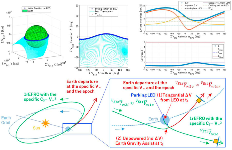
To derive conditions of 1rPFRO, a sphere whose radius is the desired $V_{\infty }$ is placed at the center of the subject planet. Then, the inverse vector of the planet’s orbital velocity vector ${\overrightarrow{V}}_B$ is placed from the planet center and a sphere of radius $‖{\overrightarrow{V}}_B‖$ is drawn, centered on the obtained vector’s tip position. The circular ring at the intersection of those two spheres yields the directions of ${\overrightarrow{V}}_{\infty }$ satisfying the insertion to 1rPFRO. The aforementioned description is visualized at the bottom of Figure 1, taking the Earth as the target object as an example.

FIGURE 1

FIGURE 1. Inertial coordinate frame ${\Sigma V}_{Bt}$ defined by position ${\overrightarrow{R}}_{Bt}$ and velocity ${\overrightarrow{V}}_{Bt}$ at epoch t of the planetary body and V-infinity vector ${}^{V_{Bt}}{\overrightarrow{V}}_{\infty }$ expressed by azimuth $\alpha$ and elevation $\delta$ (top-left), the definition of LEO’s orbital elements (${}^{V_{Et}}{i}_{LEO}$, ${}^{V_{Et}}{\Omega }_{LEO},{}^{V_{Et}}{a}_{LEO}$) with respect to the inertial frame $\Sigma V_{Et}$ (top-right), and the example of the visualized circular ring representing the directions of ${\overrightarrow{V}}_{\infty }$ satisfying the insertion to 1rEFRO (bottom).

2.3 Definition of flexible and economical Earth departure

This study identifies flexibility and economics as desirable Earth departure indicators for deep space missions. The objectives for each indicator are defined in the subsequent sections.

2.3.1 Parameters for flexibility

The departure epoch determines the orbital phase of the Earth; ${\overrightarrow{V}}_{\infty }$ at Earth departure varies widely in magnitude and direction depending on the target planetary bodies or the interplanetary transfer trajectories. The parameters are summarized as follows.

• Departure epoch $t_{dep}$

• Norm of the V-infinity vector $V_{\infty }=‖{\overrightarrow{V}}_{\infty }‖$

• Direction of the V-infinity vector ($\alpha$, $\delta$)

All of these parameters take arbitrary values depending on the target object’s orbit. In this study, the term “flexibility” is used when an Earth departure has smaller constraints on the values of each of the aforementioned parameters. Efficient Earth departure conditions for rendezvous or flyby missions to various minor and major bodies in the solar system are widely distributed over the aforementioned four parameters.

2.3.2 Parameters for economics

We deal with orbital maneuvers to obtain the target V-infinity vector ${\overrightarrow{V}}_{\infty }$ starting from LEO. Therefore, the economic efficiency is evaluated by the addition of the amount of delta-V implemented in each orbital maneuver. Here, the leverage L is introduced, which is defined by the following equation.

$L=\frac{V_{\infty }}{{\displaystyle \sum }_{i=1}^n\left(\left|{∆V}_{ix}\right|+\left|{∆V}_{iy}\right|+\left|{∆V}_{iz}\right|\right)-\left(\sqrt{\frac{2{\mu }_e}{r_{LEO}}}-v_{LEO}\right)}(4)$

where ${∆V}_{ix}$ ${∆V}_{iy}$ ${∆V}_{iz}$ is the delta-V for each axis in the spacecraft coordinate frame at the i-th maneuver out of n times, ${\mu }_E=G{M}_E$ is the Earth’s gravitational constant, and ($r_{LEO}$, $v_{LEO}$) is the distance and velocity of the spacecraft concerning the Earth’s center of gravity right before departing LEO. When each delta-V is implemented without division into each axis, the first term in the right-hand denominator of the aforementioned equation can be expressed as ${\displaystyle \sum }_{i=1}^n\left(‖{\overrightarrow{∆V}}_i‖\right)$. The right-hand denominator is the sum of the delta-V to obtain the desired infinite velocity vector starting from LEO, minus the required minimum delta-V to achieve orbital energy $C_3=0$ from LEO. The leverage L is the ratio of the obtained $‖{\overrightarrow{V}}_{\infty }‖$ to the sum of delta-V invested to achieve $C_3={‖{\overrightarrow{V}}_{\infty }‖}^2$ from the ideally reached $C_3=0$ from LEO. As the value can assume L > 1, it is referred to as “leverage”.

For L, we consider the case where ${\overrightarrow{V}}_{\infty }$ is ideally obtained from LEO; if we let $L_{ideal}$ be the leverage when the desired Earth departure is established by a single impulsive tangential delta-V of ${∆V}_{ideal}$ on LEO, the leverage is expressed as Eq. 4. Moreover, let $V_{esc}=\sqrt{2{\mu }_E/r_{LEO}}$ be the escape velocity on LEO.

$L_{ideal}=\frac{V_{\infty }}{\left(\sqrt{{V_{esc}}^2+{V_{\infty }}^2}-v_{LEO}\right)-\left(V_{esc}-v_{LEO}\right)}=\frac{V_{\infty }}{\sqrt{{V_{esc}}^2+{V_{\infty }}^2}-V_{esc}}=\frac{1}{V_{\infty }}\left(\sqrt{{V_{esc}}^2+{V_{\infty }}^2}+V_{esc}\right)=\frac{V_{esc}}{V_{\infty }}+\sqrt{{\left(\frac{V_{esc}}{V_{\infty }}\right)}^2+1}(5)$

As shown in the aforementioned equation, $L_{ideal}$ is expressed as a function of the LEO orbital radius $r_{LEO}$ and the desired V-infinity $V_{\infty }$. Furthermore, when expressing ${∆V}_{esc}$ as the necessary amount to obtain the escape velocity above LEO and ${∆V}_{dep}$ as the contribution to the net increase in $V_{\infty }$, each delta-V has the following relationship.

${∆V}_{ideal}={∆V}_{esc}+{∆V}_{dep}{∆V}_{esc}\equiv V_{esc}-v_{LEO}=\sqrt{\frac{2{\mu }_E}{r_{LEO}}}-v_{LEO}{∆V}_{dep}\equiv \sqrt{{V_{\infty }}^2+{V_{esc}}^2}-V_{esc}(6)$

Generally, the smaller the $V_{\infty }$ and lower the LEO’s altitude $h_{LEO}$ are, the larger the $L_{ideal}$ will be. However, the required ${∆V}_{dep}$ increases in proportion to the desired $V_{\infty }$.

3 Designing flexible and economical Earth departure from LEO

Starting from a wide range of LEOs, to achieve a high level of both flexible and economical Earth departure as defined in the previous section, this study adopts an orbital sequence comprised of a transition to 1rEFRO and a subsequent EGA after 1 year and organizes a preliminary trajectory design method in this section. Although the sequence is commonly used in multiple deep space missions, no study has explicitly organized a LEO-based trajectory design method or conducted a comprehensive survey of compatible low Earth orbital elements.

Section 3.1 first describes the major challenges in terms of flexibility and economic efficiency when departing directly from the LEO to the desired interplanetary orbit. Then, the goal and overall picture of the introduction of the aforementioned orbital sequence are presented. Section 3.2 summarizes the preliminary design methodology for the desired Earth departure from the LEO via 1rEFRO and EGA under the assumption of the unperturbed two-body problem and impulsive delta-V.

3.1 Introduction of an orbital sequence departing LEO

This section describes the adopted orbital sequence for the flexible and economical Earth departure from the LEO and its necessity.

3.1.1 General difficulties in departing LEO toward arbitral deep space destinations

There are challenges in terms of the required ΔV for a direct Earth departure from an arbitrary LEO to a transiting orbit to smaller bodies or Mars. As an example, we assume that the LEO (altitude 500 km, orbital inclination $i=31$°, the longitude of ascending node $\Omega =0$°) was obtained by the launch from the Japanese Tanegashima Space Center (TNSC). The target V-infinity vector ${\overrightarrow{V}}_{\infty tar}$ ($\alpha =156.95$°, $\delta =-45.20$°, $V_{\infty }=4.70$ km/s) is set from Hayabusa2’s first Earth swing-by on 3 December 2015. The transitions from the LEO to ${\overrightarrow{V}}_{\infty tar}$ are considered to be directly made from each point on the LEO. Assuming the two-body problem of the Earth and the spacecraft and assuming that each position in the LEO is a perigee, hyperbolic trajectories can be obtained as shown in Figure 2.

FIGURE 2

FIGURE 2. Examples of hyperbolic departure trajectories that directly transition from a specific LEO to a specific ${\overrightarrow{V}}_{\infty tar}$ (top-left, top-center). Corresponding delta-V quantities and leverage L (top-right) as well as the schematic of the adopted orbital sequence (1rEFRO-EGA) (bottom) are shown.

The in-plane and out-of-plane components of the ΔV quantity at each starting point and the leverage L were calculated based on Section 2.3.2 and are shown at the top-right side of Figure 2. The leverage L is significantly smaller than $L_{ideal}$ because the obtained hyperbolic trajectories’ orbital planes differ from the original LEO’s and the departure ΔV requires a large out-of-plane component. For the ${\overrightarrow{V}}_{\infty tar}$ direction, it is necessary to be existing in the original LEO’s orbital plane to bring L close to the ideal value shown in the figure. However, this significantly restricts possible low Earth orbital elements and hence limits the flexibility. Furthermore, because the LEO must be designed in accordance with the departure epoch $t_{dep}$ to obtain an economical direct departure toward ${\overrightarrow{V}}_{\infty tar}$, the direct departure from the arbitrary LEOs cannot ensure a both economical and flexible Earth departure to the arbitrary ${\overrightarrow{V}}_{\infty tar}$.

3.1.2 Employed orbital sequence (1rEFRO + EGA)

Therefore, this study adopts the two consecutive orbital operations shown in Figure 2 that start from an arbitrary LEO and allow a transition to an arbitrary target V-infinity vector ${\overrightarrow{V}}_{\infty tar}$ at an arbitrary time $t=t_2$. 1) First, the spacecraft implements a tangential impulsive delta-V in LEO at $t=t_1$ for the 1rEFRO insertion. 2) Second, the spacecraft transfers to ${\overrightarrow{V}}_{\infty tar}$ through a consequent EGA at $t=t_2$. The key feature of this sequence is the separation of velocity increment and direction adjustment. After obtaining the desired $V_{\infty tar}=‖{\overrightarrow{V}}_{\infty tar}‖$ in Eq. 1, the desired direction (${\alpha }_{tar}$, ${\delta }_{tar}$) is obtained in Eq. 2. The time required between 1) and 2), $t_2-t_1$, is approximately 1 year, which is the Earth’s orbital period $T_E$. The candidates of the departure time $t_1$ in (Eq. 1) are designed referring to the default epoch of $t_1$ by $t_{1\mathit{def}}=t_{2tar}-T_E$. The aim of this orbital sequence is to realize an economical Earth departure with high leverage L without compromising the arbitrariness of the orbital elements of the parking orbit, LEO, the target V-infinity vector ${\overrightarrow{V}}_{\infty tar}$, and the target departure time $t_{2tar}$.

A preliminary design method based on the Sun–spacecraft and Earth–spacecraft two-body problem is proposed in this study for designing an Earth departure trajectory that uses the aforementioned sequence, which is described in detail in this section. In the preliminary design, according to the premise of 1rEFRO, an assumption that the output V-infinity vector at $t_1$, ${{}^{V_{Et1}}\overrightarrow{V}}_{\infty 1o}$, and the input V-infinity vector at $t_2$, ${{}^{V_{Et2}}\overrightarrow{V}}_{\infty 2i}$, coincide as follows.

${V_{Et2}\overrightarrow{V}}_{\infty 2i}\approx {V_{Et1}\overrightarrow{V}}_{\infty 1o}(7)$

3.2 Preliminary trajectory design method

This section details the preliminary design method for the abovementioned orbital sequence. The reason for the term “preliminary design” is that this method treats the interplanetary orbit as a two-body problem of the center body and the spacecraft as an infinitesimal object with no perturbation. The two bodies are distinguished at each design stage of the sequence: the transition from LEO to 1rEFRO is Earth + spacecraft, 1rEFRO itself is Sun + spacecraft, and the transition from 1rEFRO to EGA is Earth + spacecraft. The preliminary design results in this section are adopted as initial guesses for the orbit design using nonlinear numerical optimization accounting for N-body dynamics in Chapter 0, and the usefulness is evaluated. In the following part of this section, necessary conditions for the preliminary design are first formulated: 1) the insertion condition from LEO to 1rEFRO by a tangential impulsive ΔV on LEO, and 2) the transition condition from 1rEFRO to ${\overrightarrow{V}}_{\infty tar}$ by EGA after 1rEFRO. The procedure of the specific preliminary design method is then explained by organizing the assumptions and input–output relations.

3.2.1 LEO to 1rEFRO transition (tangential impulsive ΔV)

Let ${\overrightarrow{V}}_{\infty 1o1rEFRO}$ denote the V-infinity vector satisfying the transition condition to 1rEFRO with the desired norm of $V_{\infty tar}$, and let $\left\{{\overrightarrow{V}}_{\infty 1o1rEFRO}\right\}$ denote its set. As explained in Section 0, the endpoints of the direction vectors in $\left\{{\overrightarrow{V}}_{\infty 1o1rEFRO}\right\}$ form a circular ring that coincides with the intersection of the two spheres. When expressed in terms of the azimuth and elevation (α, δ) on ${\Sigma V}_{Et1}$, the vector ${\overrightarrow{V}}_{\infty 1o1rEFRO}$ has a backward component (α < 0) relative to the Earth’s orbital velocity vector. Furthermore, the larger $‖{}^{V_{Et1}}{\overrightarrow{V}}_{\infty 1o1rEFRO}‖\equiv V_{\infty tar}$ is the smaller the area inside the circular ring will be. These characteristics can be read from the equations, and are presented in Section 3.2.1.1, including the derivation process of ${\overrightarrow{V}}_{\infty 1o1rEFRO}$. Then in Section 3.2.1.2, the set $\left\{{\overrightarrow{V}}_{\infty 1o1rEFRO}\right\}$ is further narrowed down to those capable of departing from a particular LEO to 1rEFRO.

3.2.1.1 Set of ${\overrightarrow{\mathrm{V}}}_{\mathit{\infty }}$ to achieve 1rEFRO insertion

First, by ${\overrightarrow{V}}_{\infty }$ expressed using the azimuth and elevation angles ($\alpha$, $\delta$) on ${\Sigma V}_{Et1}$ in Eq. 1, the orbital velocity vector of the spacecraft at time $t_1$, ${\overrightarrow{V}}_{Pt1}$, on ${\Sigma V}_{Et1}$ , can be expressed as follows:

${}^{V_{Et1}}{\overrightarrow{V}}_{Pt1}={}^{V_{Et1}}{\overrightarrow{V}}_{Et1}+{}^{V_{Et1}}{\overrightarrow{V}}_{\infty }=V_{Et1}{}^{V_{Et1}}\left\{\begin{array}{c}0\\ 1\\ 0\end{array}\right\}+V_{\infty }{}^{V_{Et1}}\left\{\begin{array}{c}\cos \delta \cos \alpha \\ \cos \delta \sin \alpha \\ \sin \delta \end{array}\right\}={}^{V_{Et1}}\left\{\begin{array}{c}{V}_{\infty }\cos \delta \cos \alpha \\ {\dot{R}}_e+V_{\infty }\cos \delta \sin \alpha \\ V_{\infty }\sin \delta \end{array}\right\}(8)$

To establish a planetary return after one orbit as 1rEFRO, the orbital period of the spacecraft must be the same as that of the subject planet. Inputting (${\alpha }_{1o}$, ${\delta }_{1o}$) as the azimuth and elevation angle that satisfy the condition of transition to 1rEFRO, the following equation holds.

$\begin{array}{l}‖{\overrightarrow{V}}_{Pt1}‖=‖{\overrightarrow{V}}_{Et1}‖\leftrightarrow {‖{\overrightarrow{V}}_{Pt1}‖}^2\\ ={‖{\overrightarrow{V}}_{Et1}‖}^2\leftrightarrow {V_{\infty }}^2{\cos }^2{\delta }_{1o}{\cos }^2{\alpha }_{1o}\hfill \\ +{\left(V_{Et1}+V_{\infty }\cos {\delta }_{1o}\sin {\alpha }_{1o}\right)}^2+{V_{\infty }}^2{\sin }^2{\delta }_{1o}\hfill \\ =V_{Et1}^2\leftrightarrow {V_{\infty }}^2+2V_{Et1}{V}_{\infty }\cos {\delta }_{1o}\sin {\alpha }_{1o}\hfill \\ =0\leftrightarrow \cos {\delta }_{1o}\sin {\alpha }_{1o}=-\frac{V_{\infty }}{2V_{Et1}}\hfill \end{array}(9)$

Because $\cos \delta \ge 0$ always holds from the domain of definition and the value range y of ${\cos }^{-1}$ is $0\le y\le \pi$, solving Eq. 9 for ${\delta }_{1o}$ yields:

$\cos {\delta }_{1o}=-\frac{V_{\infty }}{2V_{Et1}\sin {\alpha }_{1o}}\left\{\begin{array}{c}{\delta }_{1o}={\cos }^{-1}\left(-\frac{V_{\infty }}{2V_{Et1}\sin {\alpha }_{1o}}\right),when{\delta }_{1o}\ge 0\\ {\delta }_{1o}=-{\cos }^{-1}\left(-\frac{V_{\infty }}{2V_{Et1}\sin {\alpha }_{1o}}\right),when{\delta }_{1o}<0\end{array}\right.(10)$

Next, the possible range of ${\alpha }_{1o}$ is considered. Here, assuming that $V_{\infty }/2V_{Et1}\le 1$ holds as a prerequisite $\cos {\delta }_{1o}\ge 0$, the inverse function of the cosine function is a real number, and the value range y of the ${\sin }^{-1}$ function is $-\pi /2\le y\le \pi /2$. The possible range of ${\alpha }_{1o}$ can be constrained by using Eq. 10 as follows.

$0\le -\frac{V_{\infty }}{2V_{Et1}\sin {\alpha }_{1o}}\le 1\leftrightarrow -\frac{2V_{Et1}}{V_{\infty }}\le \frac{1}{\sin {\alpha }_{1o}}\le 0\leftrightarrow \sin {\alpha }_{1o}\le -\frac{V_{\infty }}{2V_{Et1}}\leftrightarrow -\pi -{\sin }^{-1}\left(-\frac{V_{\infty }}{2V_{Et1}}\right)\le {\alpha }_1\le {\sin }^{-1}\left(-\frac{V_{\infty }}{2V_{Et1}}\right)(11)$

From Eq. 10 and Eq. 11, the possible range of ${\delta }_{1o}$ can also be constrained as follows.

$\left\{\begin{array}{l}{\delta }_{1o}\le {\cos }^{-1}\left(-\frac{V_{\infty }}{2V_{Et1}}\right),when{\delta }_{1o}\ge 0\\ {\delta }_{1o}\ge -{\cos }^{-1}\left(-\frac{V_{\infty }}{2V_{Et1}}\right),when{\delta }_{1o}<0\end{array}\right.(12)$

Eq. 11 and Eq. 12 show that ${\alpha }_{1o}<0$, i.e., ${}^{V_{Et1}}{\overrightarrow{V}}_{\infty 1o1rEFRO}$ is pointing backward with respect to the Earth’s orbital velocity vector, and the larger the $‖{}^{V_{Et1}}{\overrightarrow{V}}_{\infty 1o1rEFRO}‖$ the smaller the range of possible values for (${\alpha }_{1o}$, ${\delta }_{1o}$).

3.2.1.2 Set of ${\overrightarrow{\mathrm{V}}}_{\mathit{\infty }}$ to achieve 1rEFRO from the specific LEO tangentially

A subset of $\left\{{\overrightarrow{V}}_{\infty 1o1rEFRO}\right\}$ that is capable of being inserted into 1rEFRO from a particular LEO is denoted as $\left\{{\overrightarrow{V}}_{\infty 1o1rEFROLEO}\right\}$ and is derived in the following part of this section. First, from this definition, the relation $‖{\overrightarrow{V}}_{\infty 1o1rEFROLEO}‖=‖{\overrightarrow{V}}_{\infty tar}‖\equiv V_{\infty tar}$ holds. Since, the end points of $\left\{{\overrightarrow{V}}_{\infty 1o1rEFRO}\right\}$ form a circular ring, the problem of finding the set $\left\{{\overrightarrow{V}}_{\infty 1o1rEFROLEO}\right\}$ is reduced to a geometrical analysis to find the intersections between the ring and the orbital plane of a given LEO. Hereafter, the equations will be organized in an orderly manner.

First, from this definition, the ring exists in the $Y=L_y$ plane, and its center is on the Y-axis of ${\Sigma V}_{Et}$ and let the ring’s radius be $L_r$. Together with $L_y$, they can be expressed using the V-infinity vector norm $V_{\infty tar}$ and the Earth’s orbital velocity norm $V_{Et}$ at epoch t as follows.

$L_y=\frac{{V_{\infty tar}}^2}{2V_{Et}}{L}_r=V_{\infty tar}\sqrt{1-{\left(\frac{V_{\infty tar}}{2V_{Et}}\right)}^2}(13)$

The existence of the intersections at time $t_1$ is investigated for LEO’s orbital elements (${}^{V_{Et1}}{i}_{LEO}$; ${}^{V_{Et1}}{\Omega }_{LEO}$) and the number of intersections is denoted by n. Here, we focus on the intersection line between the $Y=L_y$ plane where the ring exists, as well as LEO’s orbital plane. Based on the geometric relationship, a discriminant equation $K\left({}^{V_{Et1}}{i}_{LEO},{}^{V_{Et1}}{\Omega }_{LEO},L_y,L_r\right)$ and the relationship between K and n were investigated; the latter is determined as Eq. 14. Because the problem is to find the intersection of a ring and a plane, the maximum n-value is two, and the minimum is zero. For simplicity, (${}^{V_{Et1}}{i}_{LEO},{}^{V_{Et1}}{\Omega }_{LEO}$) are expressed as (i, Ω) in the equations in the rest of this section. We divided the problem into the following five cases.

$\left\{\begin{array}{c}n=0whenK>0\\ n=1whenK=0\\ n=2whenK<0\end{array}\right.(14)$

• Case 1: ($i=90°$)∩{($\Omega =0°$)∪($\Omega =180°$)}

As the intersection line between $Y=L_y$ and the LEO does not exist in this case, $n=0$ as well as ${}^{V_{Et1}}{\overrightarrow{V}}_{\infty 1o1rEFROLEO}\in \varnothing$.

• Case 2: ($i=90°$)∩($\Omega \ne 0°$)∩($\Omega \ne 180°$)

The intersection line between $Y=L_y$ and the LEO exists and is parallel to Z axis in this case. K and ${}^{V_{Et1}}{\overrightarrow{V}}_{\infty 1o1rEFROLEO}$ are derived as follows.

$K={\left(\frac{L_y}{\tan \mathrm{\Omega }}\right)}^2-{L_r}^2{}^{V_{Et1}}{\overrightarrow{V}}_{\infty 1o1rEFROLEO}=\left\{\begin{array}{c}-\frac{L_y}{\tan \mathrm{\Omega }}\\ -L_y\\ \pm \sqrt{-K}\end{array}\right\}(15)$

• Case 3: ($i=0°$)∪($i=180°$)

The intersection line between $Y=L_y$ and the LEO exists in this case. The line is parallel to the X-axis and the line’s Z component is zero. Therefore, it is always $n=2$, and ${}^{V_{Et1}}{\overrightarrow{V}}_{\infty 1o1rEFROLEO}$ is calculated as follows.

${}^{V_{Et1}}{\overrightarrow{V}}_{\infty 1o1rEFROLEO}=\left\{\begin{array}{c}\pm L_r\\ -L_y\\ 0\end{array}\right\}(16)$

•Case 4: ($i\ne 0°$)∩($i\ne 90°$)∩($i\ne 180°$)∩{($\Omega =0°$)∪($\Omega =180°$)}

The intersection line between $Y=L_y$ and the LEO exists in this case. The line is parallel to the X-axis, but the line’s Z component is NOT zero. K and ${}^{V_{Et1}}{\overrightarrow{V}}_{\infty 1oLEO}$ are expressed as:

$K={L_y}^2{\tan }^{2}i-{L_r}^2{}^{V_{Et1}}{\overrightarrow{V}}_{\infty 1o1rEFROLEO}=\left\{\begin{array}{c}\pm \sqrt{-K}\\ -L_y\\ -L_y\cos \mathrm{\Omega }\tan i\end{array}\right\}(17)$

•Case 5: ($i\ne 0°$)∩($i\ne 90°$)∩($i\ne 180°$)∩($\Omega \ne 0°$)∩($\Omega \ne 180°$)

The intersection between $Y=L_y$ and the LEO exists in this case, but the line is not parallel to both the X and Z axes. K and ${}^{V_{Et1}}{\overrightarrow{V}}_{\infty 1o1rEFROLEO}$ are derived as in the following equation.

$K=\frac{{\cos }^2\mathrm{\Omega }{\tan }^{2}i}{1+{\sin }^2\mathrm{\Omega }{\tan }^{2}i}{L_y}^2-{L_r}^2{}^{V_{Et1}}{\overrightarrow{V}}_{\infty 1o1rEFROLEO}=\left\{\begin{array}{c}-\frac{\sin \mathrm{\Omega }\cos \mathrm{\Omega }{\tan }^{2}i}{1+{\sin }^2\mathrm{\Omega }{\tan }^{2}i}{L}_y\pm \sqrt{\frac{-K}{1+{\sin }^2\mathrm{\Omega }{\tan }^{2}i}}\\ -L_y\\ -\sin \Omega \tan i\left(\frac{\frac{\cos \mathrm{\Omega }}{\sin \mathrm{\Omega }}}{1+{\sin }^2\mathrm{\Omega }{\tan }^{2}i}{L}_y\pm \sqrt{\frac{-K}{1+{\sin }^2\mathrm{\Omega }{\tan }^{2}i}}\right)\end{array}\right\}(18)$

Here, the set $\left\{{}^{V_{Et1}}{\overrightarrow{V}}_{\infty 1o1rEFROLEO}\right\}$ and the number n were derived. The V-infinity vectors in the set are classified in terms of their directions. There are a total of eight types of directions that satisfy 1rEFRO. For azimuth α, those satisfying $-180°\le \alpha <-90°$ are referred to as “inbound”, and those satisfying $-90°<\alpha \le 0°$ are referred to as “outbound”; the former flies inside the Earth’s orbit and then outside to make a return to Earth and the latter flies in the opposite order. In the case of $\alpha =-90°$, as the 1rEFRO orbit differs only in inclination from the Earth, the spacecraft returns after half a period. This is therefore technically identified as half-revolution EFRO (hrEFRO) rather than 1rEFRO.

For elevation δ, those with $-90°\le \delta <0°$ depart to the Southern Hemisphere against the ecliptic plane and return to Earth via the Northern Hemisphere, while those with $0°<\delta \le 90°$ fly in the inverse order. The following bullets show the total eight combinations of possible ${\overrightarrow{V}}_{\infty 1o1rEFROLEO}$ directions by classifying $\alpha$ and $\delta$. Notably, that there is no V-infinity vector that satisfies $\left(\alpha =-90°\right)\cap \left(\delta =0°\right)$.

• Type 1: Inbound (−180° < α < −90°), South first (−90°≦δ < 0°)

• Type 2: Inbound (−180° < α < −90°), in the ecliptic plane (δ = 0°)

• Type 3: Inbound (−180° < α < −90°), North first (0° < δ≦90°)

• Type 4: hrEFRO (α = −90°), South first (−90°≦δ < 0°)

• Type 5: hrEFRO (α = −90°), North first (0° < δ≦90°)

• Type 6: Outbound (−90 < α < 0), South first (−90°≦δ < 0°)

• Type 7: Outbound (−90 < α < 0), in the ecliptic plane (δ = 0°)

• Type 8: Outbound (−90 < α < 0), North first (0° < δ≦90°)

If two $\left\{{\overrightarrow{V}}_{\infty 1o1rEFROLEO}\right\}$ are obtained, then, either or both signs of (α, δ) differ in between those two V-infinity vectors considering the symmetry of the intersection by the ring and the plane. In summary, the combination can be seen from one of the following seven types of pairs: (1, 3) (1, 6) (1, 8) (2, 7) (3, 6) (3, 8) (4, 5).

3.2.2 1rEFRO to Earth departure (unpowered EGA)

After departing the LEO to 1rEFRO, the spacecraft will meet Earth again at time $t_2$, one orbital period later (approximately 1 year after $t_1$), for an EGA with no ΔV. Here, the final Earth departure target condition is ${\overrightarrow{V}}_{\infty tar}$. The input and output V-infinity vectors of the gravity assist are denoted as ${\overrightarrow{V}}_{\infty 2i}$ and ${\overrightarrow{V}}_{\infty 2o}$, respectively. Considering the important assumption of Eq. 7 according to the premise of 1rEFRO, their direction and magnitude are given by the following equations. Note that the display of the coordinate frames on the left shoulder of vectors is omitted in this section since the frame can be as long as they are an inertial coordinate frame centered on the Earth.

${\overrightarrow{V}}_{\infty 2i}={\overrightarrow{V}}_{\infty 1o1rEFROLEO},‖{\overrightarrow{V}}_{\infty 2i}‖=V_{\infty tar}{\overrightarrow{V}}_{\infty 2o}={\overrightarrow{V}}_{\infty tar},‖{\overrightarrow{V}}_{\infty 2o}‖=V_{\infty tar}\therefore ‖{\overrightarrow{V}}_{\infty 2o}‖=‖{\overrightarrow{V}}_{\infty 2i}‖=V_{\infty tar}(19)$

As the input and output V-infinity vectors in the EGA are determined, the swing-by trajectory is uniquely assessed as well. In this section, the equations to determine the validity of the perigee radius and the position vector ${\overrightarrow{r}}_{2\pi }$ when passing perigee at the epoch $t_2$ will be developed.

The swing-by trajectory derived from ${\overrightarrow{V}}_{\infty 2i}$ and ${\overrightarrow{V}}_{\infty 2o}$ is symmetrical about ${\overrightarrow{r}}_{2\pi }$. When ${\phi }_2$ is the rotation angle between the input and output V-infinity vectors, ${\overrightarrow{\widehat{S}}}_{2I}$ and ${\overrightarrow{\widehat{S}}}_{2O}$ are the unit vectors of each V-infinity vector, ${\overrightarrow{\widehat{r}}}_{2\pi }$ is the unit vector of ${\overrightarrow{r}}_{2\pi }$, and they are derived together with ${\overrightarrow{r}}_{2\pi }$ as follows.

$\begin{array}{l}{\overrightarrow{\widehat{S}}}_{2i}\equiv \frac{{\overrightarrow{V}}_{\infty 2i}}{‖{\overrightarrow{V}}_{\infty 2i}‖}=\frac{{\overrightarrow{V}}_{\infty 2i}}{V_{\infty tar}}{\overrightarrow{\widehat{S}}}_{2o}\equiv \frac{{\overrightarrow{V}}_{\infty 2o}}{‖{\overrightarrow{V}}_{\infty 2o}‖}=\frac{{\overrightarrow{V}}_{\infty 2o}}{V_{\infty tar}}\\ {\phi }_2\equiv {\cos }^{-1}\left(\frac{{\overrightarrow{V}}_{\infty 2i}\bullet {\overrightarrow{V}}_{\infty 2o}}{‖{\overrightarrow{V}}_{\infty 2i}‖‖{\overrightarrow{V}}_{\infty 2o}‖}\right)={\cos }^{-1}\left(\frac{{\overrightarrow{V}}_{\infty 2i}\bullet {\overrightarrow{V}}_{\infty 2o}}{{V_{\infty tar}}^2}\right)={\cos }^{-1}\left({\overrightarrow{\widehat{S}}}_{2i}\bullet {\overrightarrow{\widehat{S}}}_{2o}\right)\hfill \\ r_{2\pi }\equiv \frac{{\mu }_e}{V_{\infty }^2}\left(\frac{1}{\sin \frac{{\phi }_2}{2}}-1\right)\hfill \\ {\overrightarrow{\widehat{r}}}_{2\pi }\equiv \frac{{\overrightarrow{\widehat{S}}}_{2i}-{\overrightarrow{\widehat{S}}}_{2o}}{2\sin \frac{{\phi }_2}{2}}=\frac{{\overrightarrow{V}}_{\infty 2i}-{\overrightarrow{V}}_{\infty 2o}}{2V_{\infty }^2\sin \frac{{\phi }_2}{2}}{\overrightarrow{r}}_{2\pi }\equiv r_{2\pi }{\overrightarrow{\widehat{r}}}_{2\pi }\hfill \\ =\frac{{\mu }_e}{2V_{\infty }^2}\left(\frac{1}{\sin \frac{{\phi }_2}{2}}-1\right)\frac{{\overrightarrow{\widehat{S}}}_{2i}-{\overrightarrow{\widehat{S}}}_{2o}}{\sin \frac{{\phi }_2}{2}}\hfill \\ =\frac{{\mu }_e}{2V_{\infty }^4}\left(\frac{1}{\sin \frac{{\phi }_2}{2}}-1\right)\frac{{\overrightarrow{V}}_{\infty 2i}-{\overrightarrow{V}}_{\infty 2o}}{\sin \frac{{\phi }_2}{2}}\hfill \end{array}(20)$

The EGA at $t_2$ is valid when the perigee radius $r_{2\pi }$ derived in Eq. 20 falls in between the thresholds ($r_{\pi \mathit{min}}\le r_{2\pi }\le r_{\pi \mathit{max}}$). As ${\overrightarrow{V}}_{\infty 2i}={\overrightarrow{V}}_{\infty 1o}\in \left\{{\overrightarrow{V}}_{\infty 1o1rEFROLEO}\right\}$ holds as explained previously, two vectors exist as ${\overrightarrow{V}}_{\infty 2i}$ at maximum. The swing-by feasibility at time $t_2$ is checked for each ${\overrightarrow{V}}_{\infty 2i}$ to determine whether the corresponding ${\overrightarrow{V}}_{\infty 1o1rEFROLEO}$ can be selected or not.

3.2.3 Proposal of preliminary trajectory design procedure

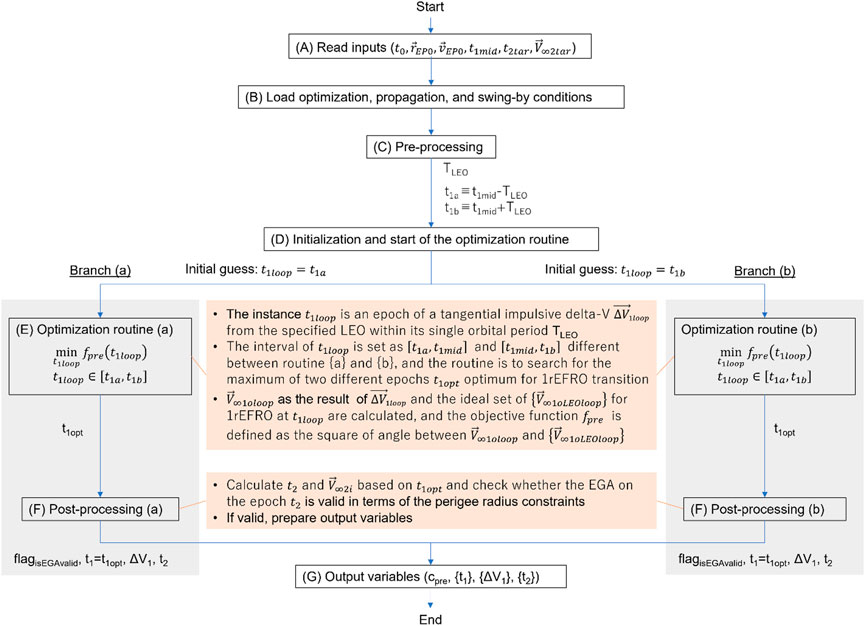
Using the relational equations derived up to the previous section based on the unperturbed two-body problem, this section proposes a preliminary orbit design procedure for an Earth departure starting from a specific LEO and going through 1rEFRO + EGA. First, if this procedure is assumed to be a function $g_{pre}$, the input–output relationship is given as follows.

$\left(\left.c_{pre},\left\{t_1\right\},{\left\{\Delta V\right.}_1\},\{t_2\right\}\right)=g_{pre}\left(t_0,{\overrightarrow{r}}_{EP0},{\overrightarrow{v}}_{EP0},t_{1mid},t_{2tar},{\overrightarrow{V}}_{\infty 2tar}\right)(21)$

As shown in the aforementioned equation, the inputs are the relative position velocity to Earth (${\overrightarrow{r}}_{EP0},{\overrightarrow{v}}_{EP0}$) in the LEO at the epoch $t_0$, the center value $t_{1mid}$ of the search range to obtain the optimum LEO-departure epochs, the target Earth departure epoch $t_{2tar}$, and the V-infinity vector ${\overrightarrow{V}}_{\infty 2tar}$. The output of the process is the epoch $t_1$, the required delta-V amount of ${\Delta V}_1$, and the final Earth departure epoch $t_2$. Assuming to obtain multiple sets of ($t_1,{\Delta V}_1,t_2$) as the result, their outputs of $g_{pre}$ are treated as the sets $\left\{t_1\},{\left\{\Delta V\right.}_1\},\{t_2\right\}$ of each variable and a number $c_{pre}$ of values exist in a set. This preliminary design procedure consists of a seven-block flow as shown in Figure 3, from (A) to (G). In block (E), the optimization routine calculates the optimum time $t_{1opt}$ at which the transition to 1rEFRO from a specific LEO is possible, and in block (F), the EGA feasibility to ${\overrightarrow{V}}_{\infty 2tar}$ at $t_2$ is evaluated. The branching in block (E) is intended to obtain $t_{1opt}$ corresponding to ${\overrightarrow{V}}_{\infty }\in \left\{{\overrightarrow{V}}_{\infty 1o1rEFROLEO}\right\}$ in each branch, where, at most, two ${\overrightarrow{V}}_{\infty }$ exist. For this reason, one of the two ends of the interval is given to each branch as the initial guess of the instance for their optimization routines. The following is a description of the process and the necessary equations for each block.

FIGURE 3

FIGURE 3. Flowchart of the preliminary design procedure of LEO-1rEFRO-EGA trajectories.

This method is referred to as “preliminary” because, as mentioned previously, it is mainly based on an unperturbed two-body problem. The specific assumptions for each phase are shown in the bullets below.

• $t_0$ to $t_1$ propagation in LEO: Earth-centered, perturbation considered

• LEO to 1rEFRO transition at $t_1$: Earth-centered, no perturbation

• 1rEFRO cruising: Sun-centered, no perturbation

• 1rEFRO to EGA at $t_2$: Earth-centered, no perturbation

By simplifying the dynamics after LEO departure to an unperturbed two-body problem, this method can simply obtain the initial design of the Earth departure-orbit starting from LEO. In contrast, from $t_0$ to $t_1$, when the spacecraft remains in the LEO, there are non-negligible variations to the orbital elements due to Earth’s higher-order gravitational potential, with third bodies such as the Moon and Sun, atmospheric drag, etc. Because the variation of LEO significantly affects the entire trajectory after LEO departure, the spacecraft state at $t_1$ is propagated with necessary perturbations.

3.2.3.1 (A) Read inputs

In this block, the conditions of the LEO ($t_0,{\overrightarrow{r}}_{EP0},{\overrightarrow{v}}_{EP0}$), the center value of search range $t_{1mid}$, and the target Earth departure conditions ($t_{2tar},{\overrightarrow{V}}_{\infty 2tar}$) are read and can be referenced in the later flows.

3.2.3.2 (B) Load propagation, optimization, and swing-by conditions

In this block, the various conditions (LEO propagation, optimization, and swing-by) are read prior to specific calculations. For the swing-by condition, the minimum and maximum perigee distances $r_{\pi \mathit{min}}$ and $r_{\pi \mathit{max}}$ are read, which will be referred to in the swing-by validation in Block (F).

3.2.3.3 (C) Pre-processing

In this block, prior to the optimization calculation in Block (E), the necessary constants are prepared through the processes. The required V-infinity vector norm for the LEO departure to 1rEFRO is the same as $‖{\overrightarrow{V}}_{\infty 2tar}‖$. The main process of this block is to prepare the interval (search range) for the instance $t_{1loop}$ of the optimization routine in Block (E). The interval is both bounded and closed expressed as $\left[t_{1a},t_{1b}\right]$. The midpoint is set to the input parameter $t_{1mid}$, and the diameter is set to the specified LEO’s orbital period $T_{LEO}$. If $t_{1mid}$ is not specified or null, the default value is calculated as $t_{1mid}=t_{1\mathit{def}}\equiv t_{2tar}-T_E$. The left- and right-bound values are prepared as follows.

$t_{1a}=t_{1mid}-T_{LEO}/2t_{1b}=t_{1mid}+T_{LEO}/2(22)$

3.2.3.4 (D) Initialization and start of optimization routines

This block initializes and starts the optimization routines (a) and (b). The difference of the routines is the initial guess of the instance $t_{1loop}$. As shown in Section 3.2.1.2, there are, at most, two directions of {${\overrightarrow{V}}_{\infty 1o1rEFRO}$} for the same LEO orbital element, and they have different departure epochs and orbital phases in the LEO. Therefore, it is intended to obtain each of two different solutions in routines (a) and (b) by starting the optimization calculations from each end of the interval, $t_{1loop}=t_{1a}$ for routine (a), and $t_{1loop}=t_{1b}$ for routine (b), with a range of the LEO’s orbital periods $T_{LEO}$ and $t_{1mid}$ as the center value.

3.2.3.5 (E) Optimization routine

In this block, the processes are performed as an optimization calculation to determine the epoch optimum as $t_1$. The main task is to calculate two independent V-infinity vectors. One is denoted as ${\overrightarrow{V}}_{\infty 1oloop}$, which is derived from the current position, and velocity vectors of the spacecraft at time $t_{1loop}$, which is an instance of the routine, considering the desired tangential impulsive delta-V of $‖{\overrightarrow{\Delta V}}_{1loop}‖$. The other is from the set ${\left\{{\overrightarrow{V}}_{\infty 1o1rEFROLEO}\right\}}_{loop}$ calculated from the osculating orbital elements ($i_{1loop}$; ${\Omega }_{1loop}$) in LEO at $t_{1loop}$ (as described in Section 3.2.1). Then, the square of the angular difference between those vectors is calculated as the objective function value of $f_{pre}$. When both V-infinity vectors are almost coincident with each other and satisfying the specified convergence conditions, the calculation is terminated, and the time $t_{1loop}$ of the latest loop is outputted as the optimal value $t_{1opt}$.

When calculating the desired, required tangential delta-V norm $‖{\overrightarrow{∆V}}_{1oloop}‖$ on LEO at $t_{1loop}$, it is derived using the known V-infinity norm $‖{\overrightarrow{V}}_{\infty 1oloop}‖=V_{\infty 2tar}$. Together with the resulting post-delta-V velocity vector ${\overrightarrow{V}}_{EP1loop}$, $‖{\overrightarrow{∆V}}_{1oloop}‖$ is calculated as follows.

$‖{\overrightarrow{∆V}}_{1loop}‖=\sqrt{{‖{\overrightarrow{V}}_{\infty 1oloop}‖}^2+\frac{2{\mu }_e}{r_{LEO}}}-‖{\overrightarrow{V}}_{EP1o}‖=\sqrt{{V_{\infty 2tar}}^2+\frac{2{\mu }_e}{r_{LEO}}}-\sqrt{\frac{{\mu }_e}{r_{LEO}}}{\overrightarrow{V}}_{EP1loop}=\frac{‖{\overrightarrow{v}}_{EP1loop}‖+‖{\overrightarrow{∆V}}_{1loop}‖}{‖{\overrightarrow{v}}_{EP1loop}‖}{\overrightarrow{v}}_{EP1loop}(23)$

The resulting V-infinity vector ${\overrightarrow{V}}_{\infty 1oloop}$ can be obtained from the post-delta-V state of the spacecraft (${\overrightarrow{r}}_{EP1loop},{\overrightarrow{V}}_{EP1loop}$) using the angular momentum vector $\overrightarrow{h}$ and Laplace vector $\overrightarrow{P}$ along the definition of an unperturbed hyperbolic trajectory as the following equations.

$\begin{array}{ll}\hfill \overrightarrow{h}=& {\overrightarrow{r}}_{EP1loop}\times {\overrightarrow{V}}_{EP1loop}\overrightarrow{P}=-\frac{{\mu }_e}{‖{\overrightarrow{r}}_{EP1loop}‖}{\overrightarrow{r}}_{EP1loop}-\overrightarrow{h}\times {\overrightarrow{V}}_{EP1loop}\overrightarrow{Q}=\overrightarrow{h}\times \overrightarrow{P}\hfill \\ \hfill & \widehat{P}=\frac{\overrightarrow{P}}{‖\overrightarrow{P}‖},\widehat{Q}=\frac{\overrightarrow{Q}}{‖\overrightarrow{Q}‖}e=\frac{‖\overrightarrow{P}‖}{{\mu }_E}{\overrightarrow{V}}_{\infty 1oloop}=‖{\overrightarrow{V}}_{\infty 1otar}‖\left(-\frac{1}{e}\widehat{P}+\sqrt{1-\frac{1}{e^2}}\widehat{Q}\right)\hfill \end{array}(24)$

3.2.3.6 (F) Post-processing

In this block, processes are performed to determine whether the target V-infinity vector ${\overrightarrow{V}}_{\infty 2tar}$ can be obtained through the Earth swing-by 1 year after $t_{1opt}$ is obtained in the previous block. The major tasks are to calculate the EGA epoch $t_2$ from $t_{1opt}$ by adding $T_E$, preparing the input and output V-infinity vectors of the swing-by considering the assumption in Eq. 7, and calculating the perigee radius $r_{2\pi }$ as described in Section 3.2.2. Then, we determine whether $r_{\pi \mathit{min}}\le r_{2\pi }\le r_{\pi \mathit{max}}$ is satisfied. If so, we assign one, and if not, we assign zero to the flag variable ${flag}_{isEGAvalid}$ and finish the processes in this block.

3.2.3.7 (G) Output variables

In this block, the results of blocks (E) and (F) in the two branches (a) and (b) are checked, respectively, and the output variables for the entire procedure are prepared. First, we initialize the integer variable that stores the number of preliminary solutions by $c_{pre}=0$, then for each branch, if ${flag}_{isEGAvalid}=1$ then increment $c_{pre}$ and store the variables to the set $\left\{t_1\right\},\left\{{∆V}_1\right\},\left\{t_2\right\}$ (note that if the results are common among both branches, count as 1), and finally, the output variables are returned.

4 Comprehensiveness of LEO as a parking orbit toward various deep space missions

Based on the methods outlined previously, this section illustrates that the 1rEFRO + EGA orbital sequence can realize a flexible Earth departure for deep space economically from an extremely wide range of LEOs. First,” ${\Sigma \mathrm{V}}_{Et}$ LEO i-Ω Diagram” is newly proposed as an indicator to explain LEO’s comprehensiveness toward deep space. The explanation of the diagram together with its usage is given in the following part of this chapter. Then, LEO is redefined as a parking orbit for various deep space missions, and its utilization is described.

4.1 Coverage of ${\overrightarrow{\mathrm{V}}}_{\mathit{\infty }\mathrm{2}\mathrm{°}}$ directions achievable by the LEO-1rEFRO-EGA sequence

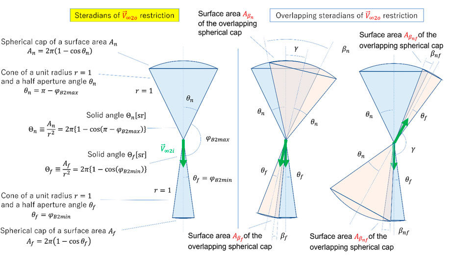
For the EGA at $t_2$, using the norm of a V-infinity vector $‖{\overrightarrow{V}}_{\infty 2i}‖=V_{\infty tar}$, the minimum perigee distance $r_{\pi \mathit{min}}$, the maximum perigee distance $r_{\pi \mathit{max}}$, and the Earth gravity constant ${\mu }_E$, the maximum value ${\phi }_{2\mathit{max}}$, and minimum value ${\phi }_{2\mathit{min}}$ of the rotating angle ${\phi }_2$ of the swing-by can be calculated as follows.

${\phi }_{2\mathit{max}}=2{\sin }^{-1}\left(\frac{1}{1+\frac{r_{\pi \mathit{min}}{V}_{\infty tar}^2}{{\mu }_E}}\right){\phi }_{2\mathit{min}}=2{\sin }^{-1}\left(\frac{1}{1+\frac{r_{\pi \mathit{max}}{V}_{\infty tar}^2}{{\mu }_E}}\right){\phi }_{2\mathit{min}}\le {\phi }_2\le {\phi }_{2\mathit{max}}(25)$

This means that the set $\left\{{\overrightarrow{V}}_{\infty 2o}\right\}$ of ${\overrightarrow{V}}_{\infty }$ that can be assumed after the EGA at $t_2$ is the set of vectors obtained by rotating $\left\{{\overrightarrow{V}}_{\infty 2i}\right\}$ around an arbitrary axis by minimum ${\phi }_{2\mathit{min}}$ and maximum ${\phi }_{2\mathit{max}}$ degrees, respectively. Let the fraction of directions that can be taken as {$\left.{\overrightarrow{V}}_{\infty 2o}\right\}$ occupying the unit sphere be defined as ${\overrightarrow{V}}_{\infty 2o}$ coverage and denoted by $c_{cov}\in \left[\mathrm{0,1}\right]$. The rest of this section givesthe description to calculate the fraction from the given ${\overrightarrow{V}}_{\infty 2i}$.

First, for a given ${\overrightarrow{V}}_{\infty 2i}$, the directions that cannot be transitioned due to the perigee restriction are defined as “Steradians of ${\overrightarrow{V}}_{\infty 2o}$ restriction” and are illustrated in Figure 4.

FIGURE 4

FIGURE 4. Schematic image of steradians of ${\overrightarrow{V}}_{\infty 2o}$ restriction for given ${\overrightarrow{V}}_{\infty 2i}$ (left) and surface areas $A_{{\beta }_n},A_{{\beta }_f},A_{{\beta }_{nf}}$ of the overlapping steradians of ${\overrightarrow{V}}_{\infty 2o}$ restriction for given set of ${\overrightarrow{V}}_{\infty 2i}$ (right).

For a given ${\overrightarrow{V}}_{\infty 2i}$, it is not possible to transition in the direction of half-peak angle ${\theta }_n$ (solid angle ${\Theta }_f$) in the reverse direction and half-peak angle ${\theta }_f$ (solid angle ${\Theta }_f$) in the forward direction. As there are, at most, two possible ${\overrightarrow{V}}_{\infty }$ from a particular LEO to 1rEFRO, the number of vectors $c_{pre}$ in $\left\{{\overrightarrow{V}}_{\infty 2i}\right\}$ that can be taken for a given LEO is (0, 1, 2). When $c_{pre}=0$, the EGA at $t_2$ is likewise not satisfied, and $c_{cov}=0$. When $c_{pre}=1$, using the surface areas $A_n$ and $A_f$ of the resulting steradians of ${\overrightarrow{V}}_{\infty 2o}$ restriction by given ${\overrightarrow{V}}_{\infty 2i}$, $c_{cov}$ is calculated as follows.

$c_{cov}=1-\frac{A_n+A_f}{4\pi }(26)$

Then, when $c_{pre}=2$, the ${\overrightarrow{V}}_{\infty 2o}$ infeasible direction for one ${\overrightarrow{V}}_{\infty 2i}$ might be the feasible direction of ${\overrightarrow{V}}_{\infty 2o}$ for the other ${\overrightarrow{V}}_{\infty 2i}$. Therefore, in calculating $c_{cov}$, the sum of the overlapped surface area of the steradians of ${\overrightarrow{V}}_{\infty 2o}$ restriction from both given ${\overrightarrow{V}}_{\infty 2i}$ is necessary. There are three possible types of overlaps, and the overlapped surface areas are denoted as $A_{{\beta }_n},A_{{\beta }_f},A_{{\beta }_{nf}}$, as shown in Figure 4. In calculating each surface area, the angles ${\beta }_n,{\beta }_f,{\beta }_{nf}$ at which the circumferences of the cones overlap inside the cross-section cut by the plane stretched by both ${\overrightarrow{V}}_{\infty 2i}$ are calculated, and the area of the overlapping spherical cap can be calculated through spherical trigonometry. Finally, $c_{cov}$ is given by using the overlapped surface areas $A_{{\beta }_n},A_{{\beta }_f},A_{{\beta }_{nf}}$ of the spherical caps as the following equation.

$c_{cov}=1-\frac{A_{{\beta }_n}+A_{{\beta }_f}+2A_{{\beta }_{nf}}}{4\pi }(27)$

4.2 Introduction of ${\Sigma \mathrm{V}}_{Et}$ LEO i-Ω diagram

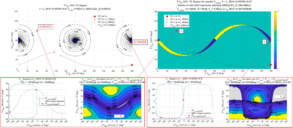
The variable $c_{cov}$ is an indicator that simultaneously expresses: 1) whether the transfer from LEO to 1rEFRO at $t_1$ is capable or not, and 2) the percentage of directions achievable by EGA at $t_2$. The variable takes the LEO’s orbital elements (${}^{V_{Et1}}{i}_{LEO},{}^{V_{Et1}}{\Omega }_{LEO}$), the departure epoch $t_1$ from LEO, and $V_{\infty tar}$ as its arguments. Since LEO is a circular orbit, the elements that determine the orientation of the orbit in inertial space can be limited to two: the inclination angle i and the longitude of the ascending node Ω. Therefore, in comprehensively understanding $c_{cov}$ for the possible LEOs, this section considers calculating the $c_{cov}\left({}^{V_{Et1}}{i}_{LEO},{}^{V_{Et1}}{\Omega }_{LEO},V_{\infty tar},t_1\right)$ against a given $t_1$ and desired $V_{\infty tar}$ across the defined ranges of ${}^{V_{Et1}}{i}_{LEO}$ and ${}^{V_{Et1}}{\Omega }_{LEO}$ ($0°\le {}^{V_{Et1}}{i}_{LEO}\le 180°$; $0°\le {}^{V_{Et1}}{\Omega }_{LEO}<360°$) to investigate the sensitivity of $c_{cov}$ across the possible i and Ω. The obtained $c_{cov}$ array, plotting the horizontal axis ${}^{V_{Et1}}{\Omega }_{LEO}$ and vertical axis ${}^{V_{Et1}}{i}_{LEO}$, is the newly proposed diagram in this study, referred to as” ${\Sigma \mathrm{V}}_{Et}$ LEO i-Ω Diagram” and shown in the upper part of Figure 5. A $c_{cov}$ contour centered at ($i_{LEO},{\Omega }_{LEO}$) = (90$°$, 0$°$), (180$°$, 90$°$) is observed in the plane stretched by the LEO’s orbital elements ($i_{LEO},{\Omega }_{LEO}$). The perigee altitude constraint adopted in this calculation is $500\le h_{\pi }\le 1e^6\mathrm{k}\mathrm{m}$. The blue-filled area of ± about 4.5$°$ from each center point implies $c_{cov}=0$ having no ${\overrightarrow{V}}_{\infty 2o}$ solution due to the infeasibility to enter 1rEFRO inside the LEO’s orbital plane. In the process of creating the diagram, the $V_{\infty }$ diagrams at $t_1$ and $t_2$ for each of the ($i_{LEO},{\Omega }_{LEO}$) points can be drawn and are shown in the red boxes in Figure 5. The left diagram in each red box shows {${\overrightarrow{V}}_{\infty 1o1rEFROLEO}$} calculated at $t_1$. In the right diagram in each red box, {${\overrightarrow{V}}_{\infty 2o}$} is identified among the 4π steradians centered at the Earth that satisfy the perigee altitude constraint at $t_2$, and a contour map of its perigee altitude $h_{\pi }$ is drawn. In contrast to the right diagram in the left red box, indicating $c_{cov}\approx 0.99$, the right diagram in the right red box has a lower value of $c_{cov}\approx 0.79$. This is because the gray-colored ${\overrightarrow{V}}_{\infty 2o}$ infeasible region largely exists due to the minimum $h_{\pi }$ constraint.

FIGURE 5

FIGURE 5. ${\Sigma \mathrm{V}}_{Et}$ LEO i-Ω diagram (top left) and the diagram for specific ${\overrightarrow{V}}_{\infty 2tar}$ (top-right) at $t=t_1$ both overlayed with LEO propagated for $\pm$ 20 days around $t_1$, and two examples of associated $V_{\infty }$ diagrams at $t_1$ and $t_2$ for specific LEO ($i,\Omega$) of (120 $°$, 60 $°$) [deg] (bottom left) and (85 $°$, 355 $°$)[deg] (bottom right).

The advantage of the ${\Sigma \mathrm{V}}_{Et}$ LEO i-Ω diagram is that it can be used to determine whether to depart from the LEO orbit in a simplified manner or not. For the diagram in Figure 5, the time history of LEO’s orbital elements propagated along ±20 days from $t_1$ with consideration of the perturbation is overlayed. The reference value of $c_{cov}$ can be checked when the departure time is shifted from $t_1$.

To evaluate the feasibility of the 1rEFRO-EGA sequence in a more straightforward manner, the top right plot in Figure 5 shows the ${\Sigma \mathrm{V}}_{Et}$ LEO i-Ω diagram for specific ${\overrightarrow{V}}_{\infty 2tar}$. In the figure, as an alternative to the aforementioned $c_{cov}$ values, it plots the number $c_{val}=\left(\mathrm{0,1,2}\right)$ of orbital solutions that is feasible for transferring to a desired ${\overrightarrow{V}}_{\infty 2tar}$ and the time history of LEO’s propagated (i, Ω) is overlayed. In Figure 5, $c_{val}=1$ holds for most of the propagation periods, which means that there is one orbital solution that is feasible up to the EGA even if the LEO departure time $t_1$ is shifted. This is because the time variation of the diagram is small when the eccentricity of the subject planet’s orbit is close to zero.

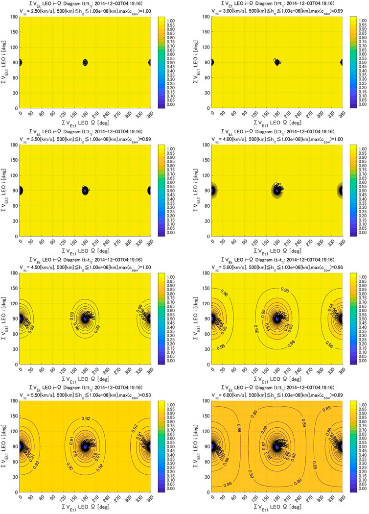
4.3 Comprehensiveness of LEO when applying the 1rEFRO + EGA sequence

Figure 6 shows the results of the ${\Sigma \mathrm{V}}_{Et}$ LEO i-Ω diagram for multiple $V_{\infty }$, while the conditions of $t_1$ and the constraint of $h_{\pi }$ are unchanged. As $V_{\infty }$ increases, $c_{cov}$ gradually decreases; however, $c_{cov}>0.85$ is satisfied in most of the areas even at $V_{\infty }=6\mathrm{k}\mathrm{m}/\mathrm{s}$. Hence, by going through 1rEFRO + EGA from most of the LEOs, the feasible ${\overrightarrow{V}}_{\infty 2o}$ direction on the unit sphere is 100% at $V_{\infty }=2.5\mathrm{k}\mathrm{m}/\mathrm{s}$ and >85% at $V_{\infty }=6\mathrm{k}\mathrm{m}/\mathrm{s}$. Although it depends on the $h_{\pi }$ constraint, the range set of $500\le h_{\pi }\le 1e^6\mathrm{k}\mathrm{m}$ is realistic in the actual mission by having an opportunity of deep space maneuver during the period of 1rEFRO.

FIGURE 6

FIGURE 6. Comparison of the ${\Sigma \mathrm{V}}_{Et}$ LEO i-Ω diagram for various $V_{\infty 2tar}\in \left\{\mathrm{2.5,3.0},\dots ,6.0\right\}\mathrm{k}\mathrm{m}/\mathrm{s}$.

These results demonstrate the comprehensiveness of LEOs by introducing the sequence 1rEFRO + EGA. It is possible to economically depart from the LEO to deep space and achieve an interplanetary orbit by a very wide $\left\{{\overrightarrow{V}}_{\infty 2o}\right\}$. In addition to the flexibility of $\left\{{\overrightarrow{V}}_{\infty 2o}\right\}$, the possible timing of departures can be as frequent as twice during the LEO’s orbital period, or twice in about 90 min for a 500 km altitude LEO. This provides a high level of time-flexibility compared to the launch window of deep space missions, which generally allows several days for the shift. These results imply that LEOs have great potential as parking orbits capable of hosting a variety of deep space missions economically.

4.4 Re-definition of LEO as a parking orbit for various interplanetary missions

As described in the previous section, the adoption of the 1rEFRO + EGA sequence used in this study has shown that economical and flexible Earth departures from a very wide range of LEOs to any ${\overrightarrow{V}}_{\infty }$ are possible. This means that LEO, which was thought to be highly constrained for interplanetary Earth departures as described in Section 3.1.1, can be used flexibly and economically as a parking orbit. The following applications are given as examples.

• Multiple deep space probes launched to the LEO by rideshare can independently depart from the LEO to their own interplanetary mission.

• Interplanetary Earth departure by a piggy-back deep space probe on an Earth observation satellite mission.

• Earth departure from a manned space station in the LEO.

• Extremely flexible launch window of the deep space probe to LEO can significantly relax the launch date and time constraints for a launch vehicle.

In utilizing LEO as a parking orbit, consideration must be given to the satellites’ congestion currently in progress in LEO due to the deployment of large-scale constellations. The congestion of LEO affects the probability of colliding with other spacecraft when staying in low earth parking orbit and during the EGA after 1rEFRO. There are several possible measures to this issue. The first is to perform a collision avoidance orbital maneuver for both during the LEO stay and the EGA. When the probability exceeds a certain level, collisions can be avoided by planning and performing a small ΔV in advance. The second is to avoid specific congested LEOs by adjusting the altitude of the parking orbit. A change in the LEO’s altitude affects the ideal leverage value $L_{ideal}$ of the entire sequence. For example, assuming an Earth departure $V_{\infty }=4\mathrm{k}\mathrm{m}$, $L_{ideal}=5.64$ at an altitude of 300 km (orbit radius 6,678 km), $L_{ideal}=5.56$ at a 500 km altitude mainly discussed in this study, and $L_{ideal}=5.38$ at 1,000 km. $L_{ideal}$ decreases when selecting the higher-altitude LEO but still provides significant leverage. Therefore, it can be said that it is possible to avoid congested LEO by changing the altitude without a significant sacrifice of economic efficiency.

5 Validation of preliminary design method

Based on the initial solution obtained by the preliminary orbit design method proposed in Section 3, we construct a detailed orbit design by numerical optimization using multi-body propagation to validate the usefulness of the initial solution and the method. First, the procedure of the detailed design method is described. Then, the LEO-rideshared asteroid exploration mission is tentatively set up, and the results of the detailed design and the discussions are presented.

5.1 Detailed trajectory design procedure

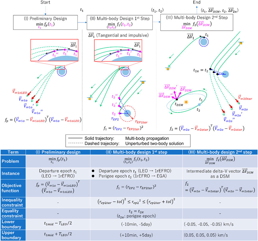
We describe the detailed orbit design method constructed to verify the initial solution obtained in Section 3. Nonlinear numerical optimization based on orbit propagation in a multi-body dynamical model is used to generate a reference orbit of 1rEFRO + EGA starting from a specific LEO from the departure epoch of $t_1$ to the perigee passage epoch $t_2$ during the EGA. The three phases that comprise this procedure and the instances of optimization and objective function at each phase are shown in Figure 7, together with an illustration.

FIGURE 7

FIGURE 7. Flowchart of the detailed trajectory design procedure composed of preliminary, multi-body first step, and the multi-body second step design phases (top) and the specifications of the optimization routine in each phase (bottom).

In phase (I), the initial solution of $t_1$ is obtained through the preliminary design method. Then, from the viewpoint of convergence, the multi-body design is achieved in two steps of phases (II) and (III), respectively.

In phase (II) as Step 1, $t_1$ and $t_2$ are taken as instances, and the objective function $f_1$ is defined as the square of the difference between the Earth–spacecraft distance and the target distance $r_{EP2tar}$ at $t_2$. The perigee distance expected in the EGA from phase (I) is substituted in $r_{EP2tar}$. The amount of tangential ΔV to be done at $t_1$ is the constant necessary to obtain the desired V-infinity vector norm under the assumption of the Earth–spacecraft two-body problem.

In phase (III) as Step 2, the deep space maneuver ${\overrightarrow{∆V}}_{DSM}$, implemented at the intermediate epoch $t_{dsm}=\left(t_2-t_1\right)/2$, is set as an instance, with $t_1$ and $t_2$ obtained in the previous step and fixed as the orbit propagation period. ${\overrightarrow{∆V}}_{DSM}$ has components in three orthogonal directions in inertial space. In this step, the objective function $f_2$ is the sum of the squares of the difference between the infinite velocity vector ${\overrightarrow{V}}_{\infty 2o}$ calculated from the spacecraft state at $t_2$ by using the two-body solution and the target V-infinity vector ${\overrightarrow{V}}_{\infty 2otar}$. The slight difference (${\overrightarrow{V}}_{\infty 2o}-{\overrightarrow{V}}_{\infty 2otar}$) at the completion of phase (III) optimization is converted into a delta-V ${\overrightarrow{∆V}}_{2\pi }$ at the perigee passage epoch $t_{2\pi }$, also by a two-body solution.

The specifications of the optimization routine in each phase are shown in Figure 7 as well. In phases (I) and (III), no equality or inequality constraints are imposed, and only a range constraint is set. In phase (II), the inequality constraint is that the Earth’s distance at time $t_2$ must be within a specified tolerance (about 10 km) about the target value of $r_{EP2tar}$, and the equality constraint is that $t_2$ must coincide with the time of the perigee passage. The range constraint values in the table in Figure 7 are examples.

5.2 Results and discussions

Reference orbits for multiple deep space probes starting from the same specific LEO are generated based on the detailed design method described in the previous section. The results are compared with those of the preliminary design, and the efficiency of paid ΔV to obtain the target V-infinity vector is evaluated in terms of leverage L.

5.2.1 LEO-rideshared asteroid exploration missions

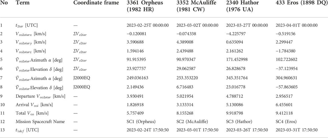
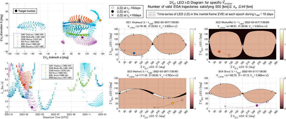
This section provides an overview of the LEO-rideshare asteroid exploration mission group originating in the LEO. The interplanetary missions will be individual rendezvous or flyby missions by four spacecraft targeting a total of four bodies each (3361 Orpheus, 3352 McAuliffe, 2340 Hathor, and 433 Eros). Table 1 shows the target V-infinity vector ${\overrightarrow{V}}_{\infty 2otar}$ at the target departure epoch $t_{2tar}$ for each asteroid. The default LEO departure time $t_{1\mathit{def}}$ is defined as the target departure time $t_{2tar}$ minus one sidereal year (365.25636 days) and is used during the design process and evaluation.

TABLE 1

TABLE 1. Target bodies and departure conditions of LEO-rideshare interplanetary missions.

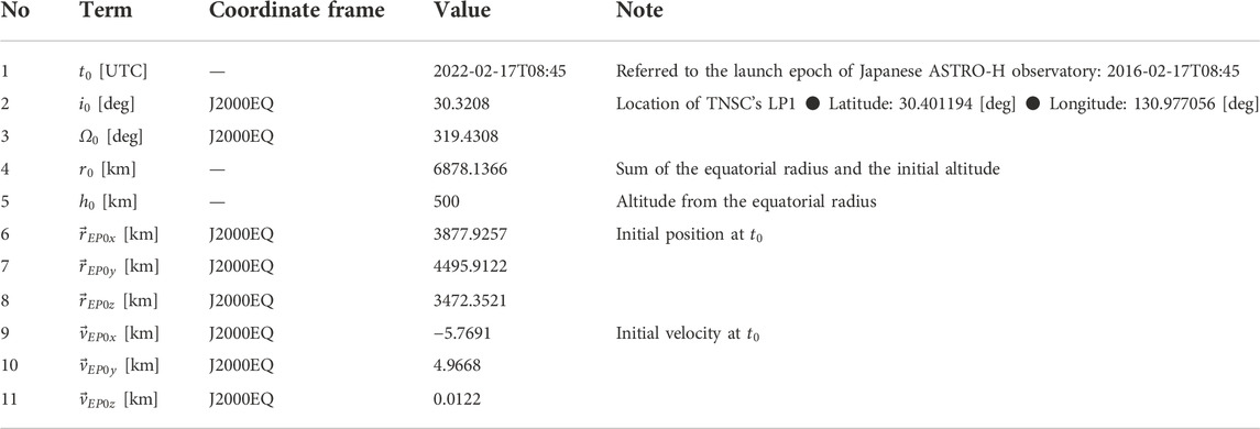
This mission is a series of LEO-rideshare asteroid exploration missions where four spacecraft are launched to the LEO from the Tanegashima Space Center (TNSC) in Japan by using the same single launch vehicle. All four use the 1rEFRO + EGA sequence adopted in this study, but depart from the LEO at different epochs each. The launch date to the LEO was set to more than 1 year before $t_{2tar}$ of 3361 Orpheus, which has the earliest target departure epoch. Table 2 summarizes the initial conditions of the LEO. The initial epoch $t_0$ was set considering the possible time in past launch achievements. The initial state (position and velocity vector) on the J2000EQ inertial frame was calculated considering the latitude and longitude of the TKSC launch pad 1 (LP1).

TABLE 2

TABLE 2. Initial conditions of the LEO parking orbit.

A ${\Sigma V}_{Et}$ LEO i-Ω diagram for specific ${\overrightarrow{V}}_{\infty 2tar}$ for each target ${\overrightarrow{V}}_{\infty 2tar}$ at the default LEO departure time $t_{1\mathit{def}}$ of each spacecraft was created, as shown in Figure 8. The propagated LEO for a $t_{1\mathit{def}}\pm 10\mathrm{d}\mathrm{a}\mathrm{y}$ period is overlayed, and a preliminary evaluation was made for each spacecraft to determine whether it would be feasible to depart. The perigee constraint at EGA was set to $500\mathrm{k}\mathrm{m}\le h_{2\pi }\le \mathit{Inf}\left[\mathrm{k}\mathrm{m}\right]$, as the actual impact on the maximum side was limited. Consequently, all four probes were found to have at least one orbit solution at $t_{1\mathit{def}}\pm 7\mathrm{d}\mathrm{a}\mathrm{y}s$ in terms of the preliminary design.

FIGURE 8

FIGURE 8. Earth departure conditions for near-Earth asteroids including four target bodies (left) and the ${\Sigma \mathrm{V}}_{Et}$ LEO i-Ω diagram for specific ${\overrightarrow{V}}_{\infty 2tar}$ at $t=t_{1\mathit{def}}$ of each spacecraft overlayed with LEO propagated for $\pm$ 10 days around $t_{1\mathit{def}}$ (right).

5.2.2 Detailed design and validation results

This section presents the results of the detailed design presented in Section 5.1 for the initial conditions and goals established in the previous section. The validity of the proposed method is evaluated by comparing the results of the preliminary design proposed in this study with those of the multi-body design. For the propagation of the LEO, the Earth is assumed as the central body, the 4 × 4 spherical harmonics model is adopted as the Earth’s gravity model, and the Sun and Moon are considered as third-body gravitational perturbations. Atmospheric drag and other perturbations were ignored. For the propagation of interplanetary orbits, the Sun (point mass) is assumed as the central body, and the Earth and the Moon are considered as third-body perturbations. Solar-radiation pressure and other perturbations were ignored.

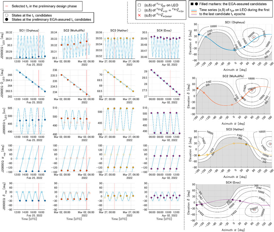
First, the spacecraft positions and orbital elements at several candidate epochs of the LEO’s departure time $t_1$ are shown in Figure 9 for each spacecraft with respect to the J2000EQ inertial frame. Each marker indicates the candidate’s departure time, and a filled marker is an EGA-assured candidate as a result of the preliminary design. The selected epochs as the output of the detailed design are indicated by the red line. As shown in the figure, there are two candidate departures per single orbital period of LEO, and one candidate per orbital period for SC1 to SC3 and the two candidates for SC4 are determined to be preliminarily EGA-assured. The basis of this decision is shown in the $V_{\infty }$ diagram in the right-hand side of Figure 9. In addition to the spacecraft’s position at each $t_1$ candidate and the direction (α, δ) of ${\overrightarrow{V}}_{\infty 1o}$ resulting from the departure, the perigee altitude $h_{2\pi }$ expected for the transition to ${\overrightarrow{V}}_{\infty 2tar}$ at time $t_2$ is plotted along (α, δ). Because the V-infinity vector ${\overrightarrow{V}}_{\infty 1o}$, indicated by the circled markers, coincides with ${\overrightarrow{V}}_{\infty 2i}$ by definition, the EGA is valid (filled-circle markers) if the circled marker is not within the grey shaded area.

FIGURE 9

FIGURE 9. States on LEO during the first to last $t_1$ candidate epochs for each spacecraft (left) and $V_{\infty }$ diagrams at $t_1$ and $t_2$ overlayed for each spacecraft as the results of the preliminary design (right).

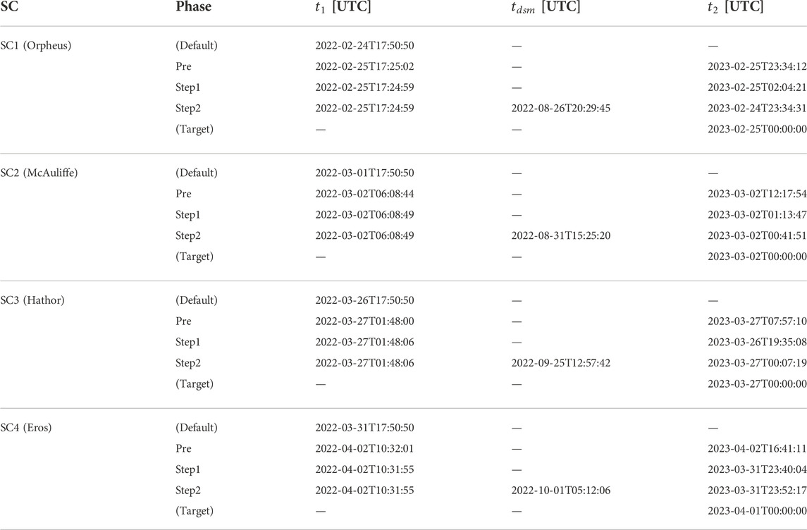
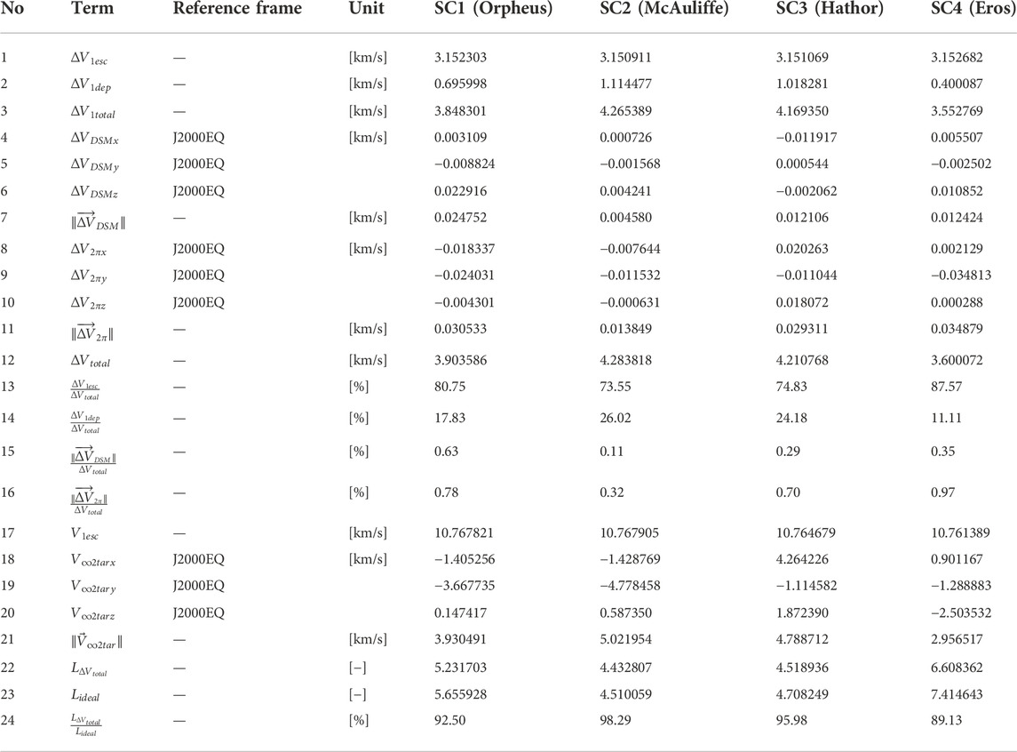
As a result of the detailed design including the multi-body design phases, the resulting epochs are shown in Table 3. For the final selected orbit solution, $t_1$, $t_{dsm}$, and $t_2$ obtained in each design phase are listed as UTC times. The resulting delta-V is summarized in Table 4. At $t_1$, the amount of delta-V to achieve C3 = 0 is defined as ${∆V}_{1esc}$, and the contribution to $V_{\infty }$ is defined as ${∆V}_{1dep}$. The total amount of delta-V at $t_1$ is denoted as ${∆V}_{1total}={∆V}_{1esc}+{∆V}_{1dep}$. The delta-V of ${\overrightarrow{∆V}}_{DSM}$ and ${\overrightarrow{∆V}}_{2\pi }$ are shown by each component in the J2000EQ inertial frame, respectively; assuming that both delta-V are not divided into each axis, the norms $‖{\overrightarrow{∆V}}_{DSM}‖$ and $‖{\overrightarrow{∆V}}_{2\pi }‖$ are tabulated. The ${∆V}_{total}$ representing the total amount of ∆V required by the spacecraft is defined by the following Eq. 28. According to Eq. 4 and Eq. 5, the actual $L_{{∆V}_{total}}$ and the ideal $L_{{∆V}_{total}}$ values of leverage were calculated.

${∆V}_{total}\equiv {∆V}_{1total}+‖{\overrightarrow{∆V}}_{DSM}‖+‖{\overrightarrow{∆V}}_{2\pi }‖={∆V}_{1esc}+{∆V}_{1dep}+‖{\overrightarrow{∆V}}_{DSM}‖+‖{\overrightarrow{∆V}}_{2\pi }‖(28)$

TABLE 3

TABLE 3. Detailed trajectory design results: Epochs.

TABLE 4

TABLE 4. Detailed trajectory design results: delta-V and leverage values.

First, it must be noted that the time $t_1$ in Step 2 is within ±10 s in all four cases compared to the values obtained in the preliminary design. This indicates that the preliminary-designed $t_1$ has a higher accuracy of less than 0.2% with respect to the LEO’s orbital period of about 90 min, and is useful as initial values for estimation in the detailed design.

Next, for the leverage value, the preliminary design assumes an ideal situation where the desired ${\overrightarrow{V}}_{\infty 2tar}$ is obtained by a single tangential impulsive ∆V at time $t_1$, in which case, the leverage value is $L_{ideal}$. To adjust the EGA condition at $t_2$ to obtain ${\overrightarrow{V}}_{\infty 2tar}$, the detailed design trajectory adds a total of six degrees of freedom, ${\overrightarrow{∆V}}_{DSM}$, and ${\overrightarrow{∆V}}_{2\pi }$, and the leverage value is expected to be below the ideal value. Consequently, the amount of delta-V required to adjust the EGA conditions $‖{\overrightarrow{∆V}}_{DSM}‖$ and $‖{\overrightarrow{∆V}}_{2\pi }‖$ totaled below 60 m/s, and as a ratio compared to ${∆V}_{total}$, the value was less than 1.5%. Its efficiency is good, and the ratio of the value $L_{{∆V}_{total}}$ to the ideal leverage value $L_{ideal}$ was about 90%. The result is rather close to the ideal value, but there are still some possibilities to decrease the amount of delta-V such as optimizing the departure delta-V amount and direction at time $t_1$, or by splitting ${\overrightarrow{∆V}}_{DSM}$ into multiple opportunities.

Finally, for time $t_2$, it must be noted that the solutions displayed in Table 3 are all within $\pm T_{LEO}\approx \pm 90\min$, furthermore, they are within $\pm T_{LEO}/2\approx \pm 45\min$. This result is expected, as there is at least one favorable transition to 1rEFRO during one orbital period of LEO. Therefore, as described in Section 4.3, the detailed orbit design confirms that the LEO has a high level of flexibility in terms of the target departure time constraint.

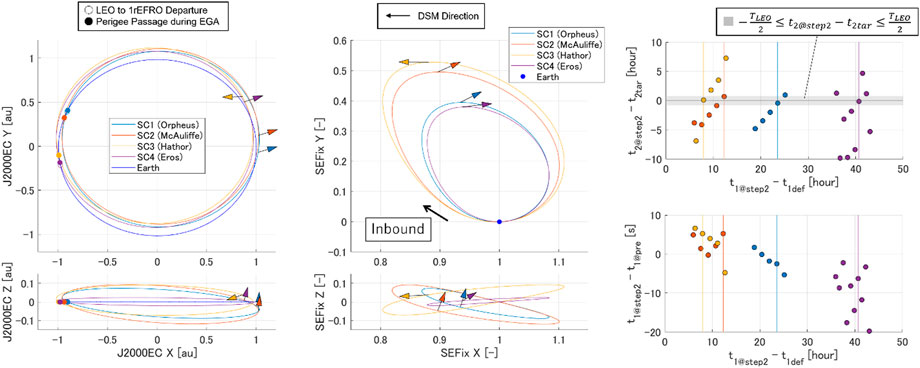
The orbit solutions obtained in the detailed design are shown in Figure 10. The left figure shows the orbit diagram expressed in the J2000EC inertial frame, and the right figure shows the diagram expressed in the Sun–Earth fixed frame. The arrow in the figure indicates the direction of DSM. As shown on the right figure, the four orbits are all inbound orbits. The left figure shows that the LEO departure position and the EGA position are almost the same, which means that the interplanetary orbit has almost the same orbital period with respect to the Earth’s. This means that the prescribed $V_{\infty }$ is appropriately not allocated to the semi-major axis that affects the orbital period, but to the eccentricity and the inclination with respect to the ecliptic plane.

FIGURE 10

FIGURE 10. Designed trajectories in the J2000EC frame (left), Sun–Earth–Fixed frame (center), and the differences of optimized time instances with respect to the references (top-right and bottom-right).

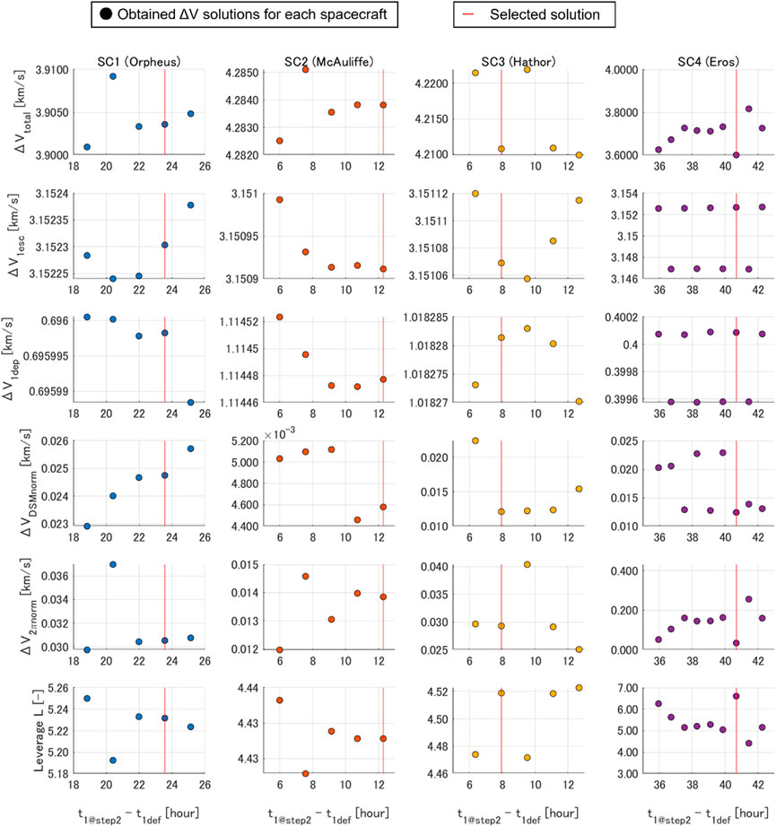
Finally, the right-hand side of Figure 10 and Figure 11 show all the results of the $t_1$ candidates. The vertical axes of the right-top and right-bottom plots in Figure 10 show the difference of $t_2$ with respect to time $t_{2tar}$ and the difference of $t_1$ in Step 2 with respect to $t_1$ of the preliminary design, respectively. The horizontal axis shows the difference of $t_1$ with respect to $t_{1\mathit{def}}$ [hours]. In Figure 11, each delta-V quantity (${∆V}_{total}$; ${∆V}_{1esc}$; ${∆V}_{1dep}$; $‖{\overrightarrow{∆V}}_{DSM}‖$, $‖{\overrightarrow{∆V}}_{2\pi }‖$) is shown on the vertical axes, with the same horizontal axis. The cases selected in Table 3 and Table 4 are highlighted in both figures as either vertical or horizontal lines. First, the right-top plot in Figure 10 shows that the cases are selected by the absolute difference of $t_2$ with respect to $t_{2tar}$ being the smallest. The right-bottom plot also shows that the differences between the $t_1$ values from the preliminary design and the Step 2 design stayed within ±20 s for all candidates, which reiterates the usefulness of the preliminary design method. In addition, the manual adjustment of $t_{mid}$ in the preliminary design to bring $t_2$ closer to $t_{2tar}$ in Step1 resulted in the plots that $t_1-t_{1\mathit{def}}$ seems to be inversely proportional to $V_{\infty }$. Qualitatively, it can be understood that a smaller $V_{\infty }$ results in a larger Earth gravity effect as a third object perturbation during the interplanetary flight; however, we leave the quantitative discussion and prediction as a subject for future work.

FIGURE 11

FIGURE 11. Obtained delta-V solutions and selected solutions for each spacecraft.

6 Conclusion

To realize a flexible and economical Earth departure from LEO, this study adopts an orbital sequence 1rEFRO + EGA to separate the increment of velocity and the directional change under the assumption of impulsive delta-V. A hypothesis was made that the orbital sequence would enable the Earth departure to interplanetary space with a high level of flexibility and economic efficiency defined in Section 2, even departing from the initial parking orbit of the LEO, which was evaluated throughout this study.

In Section 3, a preliminary design method based on unperturbed two-body dynamics is proposed, and the necessary procedures and relations are summarized. The transition from a particular LEO to 1rEFRO is reduced to a geometric problem of finding the intersection of a ring and a plane, and a discriminant equation determining the number of intersections and an analytical expression for ${\overrightarrow{V}}_{\infty }$ that enables the transition to 1rEFRO is derived. The proposed method constructs a workflow to reliably identify the maximum two directions that can transition from LEO to 1rEFRO.

In Section 4, based on the preliminary design methodology developed in the previous section, the coverage $c_{cov}$ was defined as an indicator of the flexibility of the Earth departure from the LEO. The procedure to calculate the value from the spherical cap area of the steradians of ${\overrightarrow{V}}_{\infty 2o}$ restriction is presented. The coverage is a function of the LEO’s (i, Ω), target $V_{\infty }$, and the departure epoch t from LEO. The coverage is plotted over the defined regions of (i, Ω) with given $V_{\infty }$ and t. The plot is referred to as “${\Sigma \mathrm{V}}_{Et}$ LEO i-Ω Diagram” and is proposed for the first time in this study with the aid of the preliminary orbit design. In addition to the coverage $c_{cov}$, plotting the number of feasible orbital solutions to a target ${\overrightarrow{V}}_{\infty 2tar}$ allows for a simplified and preliminary investigation of the feasibility of the Earth departure. According to the ${\Sigma \mathrm{V}}_{Et}$ LEO i-Ω diagram created with $2.5\le V_{\infty }\le 6\mathrm{k}\mathrm{m}/\mathrm{s}$ and the perigee altitude constraint set to $500\le h_{\pi }\le 1e^6\mathrm{k}\mathrm{m}$, the coverage value for most of the LEOs, excluding some polar orbits, is higher than 85%. This indicates that an extremely wide range of LEOs can realize a flexible and economical Earth departure as parking orbits together with the 1rEFRO + EGA sequence.

In this section, using the preliminary orbit design results established in Section 3 as the initial solution, a detailed orbit design was designed in three phases by nonlinear numerical optimization based on a multi-body dynamics model to evaluate the usefulness of the preliminary design method. First, an LEO-rideshare mission of four asteroid explorers was set as an example, and it was confirmed that the preliminary orbit design was valid through the ${\Sigma \mathrm{V}}_{Et}$ LEO i-Ω diagram. The detailed design results showed that the LEO departure epoch $t_1$ of all four spacecraft remained within ±10 s between the preliminary and detailed designs. This is less than 0.2% of the LEO orbital period, indicating that the preliminary design solution is useful as an initial guess for the detailed design. Furthermore, the leverage $L_{{∆V}_{total}}$ calculated from the total ∆V amount including DSM is all $L_{{∆V}_{total}}>4.4$, which is larger than about 90% of the ideal value $L_{ideal}$. Finally, it was also confirmed that the EGA epoch $t_2$ fell within the target Earth departure epoch $t_{2tar}\pm 45$ min, which possesses a high level of flexibility in terms of the Earth departure epoch.

In conclusion, this study revealed that LEO has both flexibility and economic efficiency as a parking orbit for deep space missions by adopting the 1rEFRO + EGA sequence. Based on these results, the study of a standardized deep space orbital transportation architecture starting from LEO, which is expected to significantly reduce the unit cost per launch weight in the future, can be accelerated. Also, possibilities of alternative sequences including other orbital manipulations such as powered EGA and Lunar gravity assist shall be investigated as future work.

Data availability statement

The raw data supporting the conclusion of this article will be made available by the authors, without undue reservation.

Author contributions

The work was conceptualized and developed as a collaboration among all authors. The manuscript was prepared by YTa, and the authors TS and YTs reviewed the manuscript.

Acknowledgments

The authors thank Dr. Roger Gutierrez Ramon and Mr. Manel Caballero for sharing the dataset of Earth departure conditions for rendezvous missions to various near-Earth asteroids.

Conflict of interest

The authors declare that the research was conducted in the absence of any commercial or financial relationships that could be construed as a potential conflict of interest.

Publisher’s note

All claims expressed in this article are solely those of the authors and do not necessarily represent those of their affiliated organizations, or those of the publisher, the editors, and the reviewers. Any product that may be evaluated in this article, or claim that may be made by its manufacturer, is not guaranteed or endorsed by the publisher.

References

Ikenaga, T., Utashima, M., Ishii, N., Kawakatsu, Y., and Yoshikawa, M. (2015). Interplanetary parking method and its applications. Acta Astronaut. 116, 271–281. doi:10.1016/j.actaastro.2015.07.018

CrossRef Full Text | Google Scholar

Ito, D., Pushparaj, N., and Kawakatsu, Y. (2022). Expanding interplanetary transfer opportunities from geostationary transfer orbits via Earth synchronous orbits. J. Spacecr. Rockets, 1–16. doi:10.2514/1.a35270

CrossRef Full Text | Google Scholar

Kawaguchi, J., Kuninaka, H., Fujiwara, A., and Uesugi, T. (2006). MUSES-C, its launch and early orbit operations. Acta Astronaut. 59 (8–11), 669–678. doi:10.1016/j.actaastro.2005.07.002

CrossRef Full Text | Google Scholar

Kawakatsu, Y. (2009). “v∞ direction diagram and its application to swingby design,” in Proceedings of 21st International Symposium on Space Flight Dynamics, Toulouse, France, September 28-October 2, 2009.

Google Scholar

Ozaki, N., Pushparaj, N., Takeishi, N., Hyodo, R., and Hyodo, R. (2022). Asteroid flyby cycler trajectory design using deep neural networks. J. Guid. Control, Dyn. 45 (8), 1496–1511. doi:10.2514/1.G006487

CrossRef Full Text | Google Scholar

Russell, R. P., and Ocampo, C. A. (2005). Geometric analysis of free-return trajectories following a gravity-assisted flyby. J. Spacecr. Rockets 42 (1), 138–152. doi:10.2514/1.5571

CrossRef Full Text | Google Scholar

Strange, N., Russell, R., and Buffington, B. (2007). “Mapping the V-infinity globe,” in Proceedings of AAS Astrodynamics Specialist Conference (Michigan, USA, August 19-23, 2007, : Mackinac Island), 07–277.

Google Scholar

Takahashi, S., Ogawa, N., and Kawakatsu, Y. (2019). General characteristics of free-return ensured orbit insertion and trajectory design with MOI robustness in MMX mission. Trans. Jpn. Soc. Aeronautical Space Sci. Aerosp. Technol. Jpn. 17 (3), 404–411. doi:10.2322/tastj.17.404

CrossRef Full Text | Google Scholar

Tsuda, Y., Nakazawa, S., Kushiki, K., Yoshikawa, M., Kuninaka, H., and Watanabe, S. (2016). Flight status of robotic asteroid sample return mission Hayabusa2. Acta Astronaut. 127, 702–709. doi:10.1016/j.actaastro.2016.01.027

CrossRef Full Text | Google Scholar