FPGA-Based CNN for Real-Time UAV Tracking and Detection

1 Introduction

There is an increasing interest in leisure and commercial use of UAV leading to a rise in market demand. However, there has also been an increasing rise in incidents involving UAV usage for undesirable and potentially harmful purposes. For example, airports have reported numerous cases of UAVs disturbing airline flight operations, leading to near collisions (Huttunen, 2019). Apart from airports, operation of unauthorized UAVs is an even bigger challenge around critical buildings (such as prisons, nuclear installations, and power stations) and government/military infrastructure. Manual detection and tracking of UAVs to provide 24 × 7 coverage is neither practical nor feasible. Therefore, it is an urgent need to develop automated systems that can detect and track UAV activity around key buildings and locations.

It is easy for the human brain to detect and identify objects such as UAVs; however, computer systems cannot achieve the same task without running complex algorithms, which needs be able to self-learn and adapt themselves in order to identify and track objects such as UAVs in real time. For a computer system, UAV monitoring is a difficult task because the image processing must cope with diverse and complex backgrounds in the real-world environment, plus there are numerous UAV types in the market. There are four primary techniques for locating UAVs: 1) radar 2) transmitted RF 3) acoustic sensing, and 4) visual sensing. Radars can be used to detect the location of an object in the sky but are not able to classify whether it is a UAV or not (for example a bird). The second technique looks for transmitted RF signals from the UAV, and using a directional antenna, it could compute the angle and direction of flight, but not its type. The acoustic sensing is similar to radar, but it uses interconnected microphone elements for receiving sound wave echoes. Finally, the visual sensing approach processes images or videos to estimate the position and identity a target object. In this work, we use the visual approach by leveraging the recent breakthrough in the computer vision field of neural networks (Saqib et al., 2017).

SoC-based field-programmable gate arrays (FPGA) are well suited to implement and run neural network algorithms because they provide powerful parallel computational capability with the flexibility of a reconfigurable hardware design. However, due to limited DSP hardware resources, it is quite challenging to implement floating-point arithmetic functions on FPGAs. Researchers have long circumvented this limitation by deploying NN algorithms on the processing system (PS) section of the hardware platform, rather than the programming logic (PL) section. This means that the algorithm never fully utilizes the prime benefits of achieving hardware acceleration by parallel processing on the FPGA platform. In this study, we overcome that challenge by designing a true FPGA-based system on the PL section of the hardware platform, running at full video frame rate. Our hardware-centric design approach resulted in a highly optimized, real-time SoC-based monitoring device that can identify and track illegal UAVs. Being a SoC-embedded system, the device could be small and battery-powered, making it very portable and cost-effective (Omar Salem Baans, 2019).

1.1 Contributions and Organization

The main contributions of our work are:

• to the best of our knowledge, this is the first system to use the Zynq UltraScale XCZU9EG SoC for UAV detection and tracking problems;

• we have achieved tracking and detection at full video frame rate, using the FPGA by designing our own novel processing system, compared to using a DPU IP block (as used, for example, in the Vitis Model Zoo from Xilinx);

• the system has been tested against real flying UAVs, running in real-time;

• we have the ability of loading a data set of weights from 500 k of images on the FPGA using quantization;

• novel background-differencing technique provides the location of the moving object, for the camera to track. This allows small flying objects to be detected in a cluttered environment;

• the integrated UAV monitoring system consists of a UAV detector and a motor-controlled camera, with auto focus. From the results, the integrated system outperforms the detection-only and the tracking-only subsystems;

• as far as the author is aware, this is the first Xilinx UltraScale implementation of a CNN using a custom network optimized for UAV detection, using INT8 quantization, to reduce the DSP48E2 MACC resources to a minimum while maintaining accuracy. This allows the system to be ported to a lower cost FPGA, such as the Zynq or Kintex.

The rest of this article is organized as follows. We first described the problem and proposed implementation in Section 2. The proposed UAV detection and tracking system is described in Section 3. The collected UAV datasets are introduced in Section 4. UAV tracking is presented in Section 5. Our CNN implementation is given in Section 6. The FPGA considerations are provided in Section 7. Experimental results are presented in Section 8. Concluding remarks are given in Section 9.

2 Problem Formulation and System Implementation

To detect an object, we need a method or algorithm that can recognize features of interest from a sequence of images. Traditionally, to extract features and descriptors, algorithms such as the scale invariant feature transform (SIFT) (Lee et al., 2015) were used, where the features are local and based on the appearance of the object at particular interest points. The speeded-up robust features (SURF) method carries out the task of finding point correspondences between two images of the same scene or object, and the local binary pattern (LBP) method is used to describe texture characteristics of the surfaces. These three discriminant features can be combined to form the histograms of oriented gradients (HOG) feature vector (Kher and Thakar, 2014). The advantage of the HOG algorithm is that the features can still be obtained after the object of interest has transition, changed orientation, illumination, or rescaling. This is due to the image being transformed into a large collection of local feature vectors. The HOG feature vector is obtained by computing normalized local histograms of image gradient directions or edge orientations.

Neural networks have been found to be a good alternative to this type of traditional processing. In deep learning, a CNN is a class of neural network, with multiple layers. A CNN consists of multiple convolutional and fully connected layers (i.e., multiple types of interconnected neural networks), where each layer is followed by a non-linear activation function. These networks can be trained end-to-end by back-propagation. This is of interest, as they can learn from different UAV images. We can also introduce feature extraction as a layer. The first modern CNNs that were developed in the 1990s showed us that a CNN model, which aggregates simpler features into progressively more complicated features, could be successfully used for handwritten character recognition (Lecun et al., 1998). This work has led to a lot of follow-up research on the developments and applications of deep learning methods.

Our proposed design utilizes novel technique to reduce the heavy floating-point dependency for FPGA implementation while implementing CNNs. In our design, the traditional feature transforms, and oriented gradient becomes a layer within the CNN. The big advantage of CNNs is that they can be self-learning, i.e., the more images they are subjected to, the better they are at the classification of objects, just like our brains. We consider a region of interest (ROI) guarded by a FPGA-based CNN–enabled UAV monitoring and detection system, which is composed of a single camera, an FPGA board, etc (Figure 1). For simplicity, we consider a single UAV intruder that produces a signature signal (i.e., an image) detectable by the system.

FIGURE 1

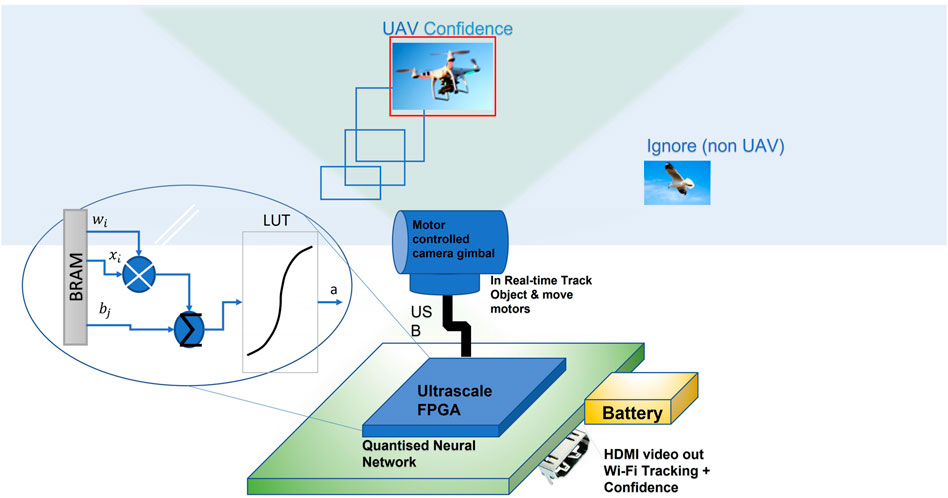
FIGURE 1. Block diagram for the proposed UAV tracking and detection system.

3 UAV Monitoring System

To realize high performance, the system consists of two modules, namely, the UAV tracking module and the neural network–based UAV detection module. The UAV detection is based on a modified CNN algorithm, designed to give the maximum FPGA performance. The tracking module uses our novel background-differencing algorithm. These two modules complement each other, and they are used jointly to provide accurate, real-time UAV detection for a given video input. The tracking allows the region of interest to be scanned. The tracking could be locked on to the incorrect object, but the CNN is used to provide a feedback path to confirm that the tracking is locked on to an object of interest. Training can be performed on a desktop PC with multiple graphics processing units (GPU), but the inference is to be performed on an FPGA. Each neural network of our CNN is structured in layers. Neurons take their values from the previous layer and create a weight sum. Each neuron calculates a weighted sum of its inputs (x). The neuron is activated by using a linear activation [Figure 2 and Eq. 1 (Rosenblatt, 1962)] followed by a rectified linear units (ReLU) function Y with a threshold detector to extract a feature. The weight connecting the i input neuron, X_i, and the j output neuron, Y_j, is denoted by w_ij. There are different types of activation functions, such as linear, sigmoid, and hyperbolic tangent, with the linear function being preferred for the FPGA as it reduces floating-point resources. The weights themselves are transferred to block random access memory (BRAM) for maximum performance. In our CNN, the same set of weights w is usually reused heavily in convolutional layers, thus forming input w_ij type of parallel multiply accumulator (MACC) operations, as shown in Figure 2.

$f=\sum _i^n{w}_{ij}{x}_i+b_j,(1)$

where w_ij is the weight for the i^th input (x_i) and j^th output neuron of the feature map, and b_j is the bias value for the j^th output neuron.

FIGURE 2

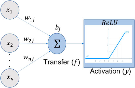
FIGURE 2. Weights (w_ij) from each input are summed up using a transfer function, Eq. 1; a bias value (b_j) is added to obtain the activation function, Eq. 2. For a convolution, every neuron has a transfer and activation function for each new feature layer.

A CNN is a network with many interconnected layers. The weights and biases are fixed during the learning process. After training, some optimization can be performed to remove unwanted layers and to compress the neurons. The CNN takes a patch of pixels or data and calculates a new value in a new feature map layer. This is repeated across the complete spatial map of the input layer. All calculations can be performed in parallel on the FPGA. As a result of this convolution (mathematical operation on two functions, processing a third), we end up with a relatively small number of weights.

$y=ReLU\left(\sum _{i=1}^n\sum _{j=1}^m{w}_{ij}{x}_{ij}+b_j\right),(2)$

where ReLU is the rectified linear units function max (0, x), i is the number of inputs, w_ij is the weight for the i^th input (x_i) and j^th output neuron of the feature map, b_j is the bias value for the j^th output neuron, and n, m values represent the size of our convolution.

4 Data Collection and Augmentation

The first step in developing the UAV monitoring system is to collect UAV flying images and videos, for the purpose of training the CNN and testing. We collected over 1,000 public domain images of UAVs. These were rescaled to a size of 227 × 227. Some of the samples of this data set are shown in Figure 3B. This was added to the ImageNet Large Scale Visual (ILSVRC) Russakovsky et al. (2015) data set of 500,000 photographs with 500 categories.

FIGURE 3

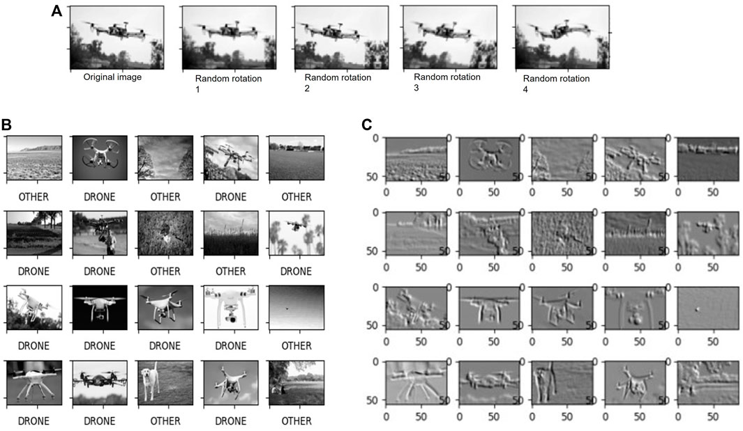
FIGURE 3. Steps involved in data collection and image augmentation. (A) Image augmentation: each image is randomly rotated at various angles to increase the training set data and enhance CNN learning. (B) Sample database for static image test of the CNN. (C) Processed images from the sample database after the first CNN convolution layers.

For playback testing, we created a video data set. This consisted of 40 video sequences that were taken outside, with different UAV models, in various locations and weather conditions. Some of these video clips contain more than one UAV, while others contain non-UAVs and birds to present more of a challenge. We also added our own video clips shots, taken locally, using three different UAV models. Several examples of the same UAVs in different appearance are shown in Figure 3B. To shoot these video clips, we considered a wide range of background scenes, camera angles, different UAV shapes, and weather conditions. They are designed to capture UAVs’ attributes in the real world such as fast motion, extreme illumination, and distance near and far. In addition, some video clips do not contain any UAVs, which we used for validation.

The duration of each video ranges from 1 min to about 15 min, and the frame resolution is 1920 × 1080. The frame rate is 30 frames per second.

To improve the data set, we took the images, resized, and rotated them at various angles. From a single image, we created more than 10 different variants. As an example, we have shown four different variants of the same drone image in Figure 3A. For the CNN training set data augmentation, each image has been slightly altered by a different rotation angle, even though they are derived from the same original image.

5 UAV Tracking

In order to obtain best possible accuracy, tracking needs to run at the full frame rate of the camera Newcombe (2012). To further improve the tracking performance, we also preprocessed the video input. This preprocessing involves subtracting the current frame from the previous frame and taking the absolute values pixel-wise to obtain the residual image of the current frame. Note that, we do the same for the three RGB channels of a color image frame to get a color residual image. If there is a panning (zoom in or out) movement of the camera, we also need to compensate for the global motion of the whole frame before the frame subtraction operation with reference to the background (B) value of the image. A numerical value of B signifies that it is an actual background (static), while a non-numerical value implies a moving object (non-static). We obtained the value of B using a modified Stauffer and Grimson algorithm (Chan et al., 2011), as shown in Eq. 3.

$B={\mathit{arg}}_{b_{\mathit{min}}}\left(\sum _{k=1}^b{\omega }_k>T\right),(3)$

where the threshold T is a measure of the minimum portion of the data that should be accounted for by the background (B), ω_k is the respective mean for the k^th Gaussian model, and b is the total number of Gaussian models. The algorithm models each pixel with a mixture of Gaussians. At every frame, for each pixel, the distance of pixel’s color value is calculated from each of the associated K Gaussian distributions (default value of K = 3). We classify a pixel as a foreground pixel based on the following two conditions:

1. If the intensity value of the pixel matches none of the K clusters (default value of K = 3).

2. If the intensity value is assigned to the same cluster for two successive frames, and the intensity values $x\left(T\right)$ and $x\left(T-1\right)$ are both outside the 50% (user adjustable) mid-range $\left(c_k-X,c_k+X\right)$.

where x is the current pixel, X is the number of pixels, c_k is the Gaussian central value, and T is the threshold value used in Eq. 3.

Since there exists strong correlation between two consecutive images, most of the background of raw images will cancel out and only the fast-moving object(s) will remain in residual images. This is especially true when the UAV is at a distance from the camera and its size is relatively small. The observed movement can be well approximated by a rigid body motion. Furthermore, if the tracker loses the UAV for a short while, there is still a good probability for the tracker to pick up the UAV, but some user intervention may be required. Also, extra time should be allowed for the camera to re-pan and focus.

The UAV detector has two tasks: first, we can use the detector to find the UAV and initialize the tracker. Typically, the UAV tracker is used to track the detected UAV after the initialization. However, the UAV tracker can also play the role of a detector when an object is too far away to be robustly detected as a UAV due to its small size. In other words, based on the distance of the object, a tracker can play the role of detector and vice versa. Second, we can use the tracker to track the object before detection based on the residual images as the input. Once the object is near, we can use the UAV detector to confirm whether it is a UAV or not.

A UAV can be detected once it is within the field of view and of a reasonable size. The detector (CNN) will report the UAV location to the tracking camera so that the camera can refocus on the object. During the tracking process, the detector keeps providing the confidence scores of a UAV at the tracked location as a reference to the tracker. The final updated location can be acquired by combining the confidence scores of the tracking and the CNN detection, as shown in Eqs 4–6 (Chen et al., 2017).

$A_d=\frac{1}{{\left(1+e^{-{\beta }_1\left(R_d{-\propto }_1\right)}\right)}^{\mathit{adj}}},(4)$

$A_t=\frac{1}{{\left(1+e^{-{\beta }_1\left(R_t{-\propto }_1\right)}\right)}^{\mathit{adj}}},(5)$

$A_f=\mathrm{m}\mathrm{a}\mathrm{x}\left(A_n,A_t\right),(6)$

where R_d is the confidence of the CNN detection; R_t denotes our tracker confidence; A_d and A_t are the confidence score of detection and tracking, respectively; A_f is the overall “Confidence” score of an UAV detection; and β₁, β₂, ∝₁, ∝₂ are acceptance threshold parameters, set by the user, which can be used while evaluating the condition statement in the UAV detection flowchart shown in Figure 4.

FIGURE 4

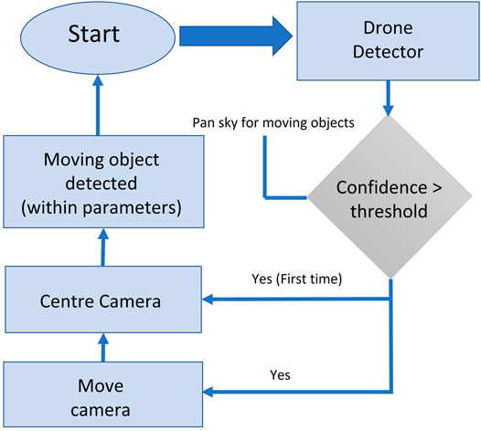
FIGURE 4. Flowchart of the proposed UAV monitoring system.

6 Proposed CNN Implementation

The goal of UAV detection is to detect and localize the UAV in video images, in real time. Our approach is built on a CNN algorithm, as shown in Figure 5. Each of the stages in this algorithm is explained in the following sections. In our model, the CNN can be applied simultaneously to multiple bounding boxes, as identified by our tracking/background-differencing algorithm. It then predicts class probabilities for those boxes. These boxes are confined to the area identified by our background-differencing algorithm, thus improving performance, compared to applying the CNN to a full frame.

FIGURE 5

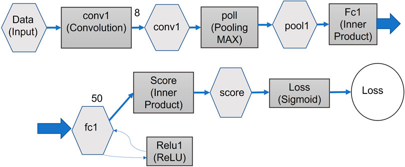
FIGURE 5. Proposed architecture of the CNN algorithm for our implementation. The algorithm has been optimized for speed versus detection performance.

Our CNN design enables end-to-end training and real-time speeds while maintaining high average precision. The CNN trains on full images and directly optimizes detection performance. This unified model has several benefits over traditional methods of object detection. First, the CNN is extremely fast. Since the FPGA sees frame detection as a regression problem, we do not need a complex pipeline of images. We simply run our neural network on a new frame image in the test. Our model unifies separate components of object detection into a single neural network. Our network uses feature extraction from the image, as identified by the “UAV Tracking” module (discussed later). Each object is examined simultaneously, detected by the tracking algorithm. This means our network can identify not only just drones but also multiple objects in the image. The images used as an input for the CNN are all rescaled for the CNN to a standard size.

We start by evaluating the CNN on our detection data set (Chollet, 2018). We discuss the details of this data set in Section 4 and Section 6.4. Our CNN consists of convolution layer, pooling layer, and fully connected layer. The initial convolution layers of the network extract features from the image (Figure 3C), while the fully connected layers predict the output probabilities and coordinates. Our network architecture was inspired by the GoogLeNet model (Das, 2020) for image classification. The difference being that our network has additional convolution layers followed by two fully connected layers. However, instead of the inception modules used by GoogLeNet, we simply used 1 reduction layer followed by 3 convolution layers, similar to the network in network (NIN) model (Mengxi et al., 2018). The full network is shown in Figure 5.

6.1 Convolution

The convolution extracts and preserves important features from the input, in a feature map. In most CNNs, the input can be of multiple layers; for example, one layer for each color. The feature map layer can also be of multiple layers. This means that when calculating the weight of each layer of the feature map, the calculation must also include all the layers of the input.

For our implementation, each pixel/data point in the second layer is calculated from a sliding patch of around 25 pixels/data points in the feature map, to produce a smaller map in the next layer. Where possible, the calculations are performed in parallel on the PL. This reduces the number of weights, compared to a fully connected network. For example, for a UAV image, the colors are on different input layers, requiring a multidimensional feature layer, as shown in Figure 6. The convolution value (yⁿ) can be calculated using Eq. 7 shown below.

$y^n=\sum _{i=1}^5\sum _{j=1}^5\sum _{k=1}^3{w}_{\mathit{ijk}}^n{x}_{\mathit{ijk}}+b_n.(7)$

FIGURE 6

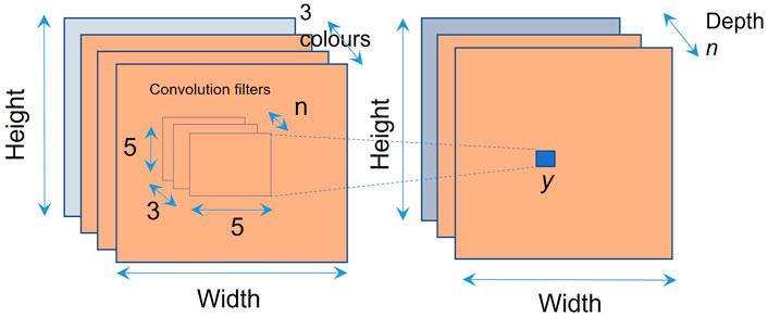
FIGURE 6. Multichannel convolution allows images of different types to be processed in parallel on the FPGA. In this example, we have chosen the optimum values of feature sizes for our FPGA implementation. These optimum values can change for different implementations. For our implementation, we have chosen n = 30 as the optimum value.

The maximum values for (i, j, k) shown in Eq. 7 and Figure 6 correspond to 25 pixels (i × j = 5 × 5) for each convolution on each one of the three RGB colors (k) in the image. For our model, we are using an optimum value of n = 30 for performance vs. number of weights.

6.2 Pooling Layer

We use a pooling layer to down sample the image (e.g., Max pooling, where we look for the maximum values, as shown in Figure 7). This compresses the image and extracts the main features. We process the downsampling in parallel on the PL on the FPGA, for maximum performance.

FIGURE 7

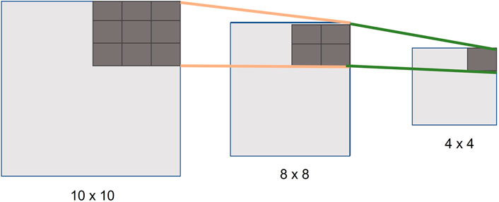
FIGURE 7. Example of how we make use of pooling layers for downsampling the images in our implementation.

6.3 Basic Multichannel CNN Convolution

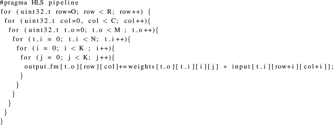
The most complex operation that needed to be accelerated was the multichannel CNN convolution. Each sum is a convolution of all the input maps. Each output map uses a different kernel. The operation can be shown as a set of loops, in pseudocode. In our case, this is coded in high-level synthesis (HLS) programming language, with loops set to pipelining, as these loops are converted to parallel operations on the FPGA (Hanif and Putra, 2018). HLS coding is discussed in greater detail in Section 7.3. For the convolution computing process, variables row and col correspond to the size of the convolution kernels, to correspond to the size of the input feature maps, and i and j represent the number of input and output feature maps. We performed unrolling on i and j. As the values of i and j increase, the number of parallel processing elements (PE) also increases. The operation in our PE is the multiplication of the input feature pixels and the corresponding weights (w). But, when i and j are large enough, the resource utilization will exceed the total number of our hardware resources, so we divided the whole calculation into several tiles to meet resource utilization as shown in Figure 8A. Note that, the order of the “loops” in Listing 1 is independent so that they can be moved around and can also be run in parallel. Where the computational requirements are too much for the FPGA, we have broken down the layers further into subtiles, as shown in Figure 8B.Where K = kernel, C = columns, TR = tile rows, R = rows, N = input maps, and M = output feature map.

FIGURE 8

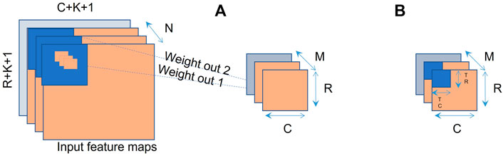
FIGURE 8. (A) Basic multichannel CNN convolution allowing for FPGA parallel acceleration. (B) Convolution layers broken down further into sub ‘tiles’ to reduce computation time, by making use of parallel processing.

Listing 1. HLS pseudocode of our FPGA convolutionAt the end of the network, a fully connected layer is applied. Each neuron in the fully connected (FC) layer is connected to all neurons in our upper layer, and the features are extracted from the previous layer and combined to function as a classifier in the CNN. As shown in Figure 5, the final step is to use the loss function, which distils all aspects of our model and results down into a single number, thus providing our weighting for calculating the score (confidence value), output prediction y_c, and measuring the distance from the truth values. The loss function can be calculated using Eq. 8.

$Loss=\sum _{c=1}^M\left(y_c\log {\widehat{y}}_c\right),(8)$

where M is the number of classes (500 in our case) and y_c is the model’s prediction for that class (c) which can be either 1 or 0.

6.4 Training the CNN

First, we collected the data, avoiding random images and using as much training data as possible (as discussed in Section 4), a created a training model, which is based on the ILSVRC data set plus our UAV data, as discussed in Section 6. We used MATLAB to create the training set, as shown in Paluszek et al. (2020). This iterates through each epoch (one complete cycle through the full training data set), until the training set is optimized. Figure 9 shows the results of the validation data (approx. 50 K images) against the test data (approx. 450 K images). We used a Broadberry GPU server TYAN Thunder FT48T-B7105 with four NVIDIA GTX 1080 Ti graphics cards to carry out the processing of the training set. Even with additional GPUs, it took a few days (11,199 min) for the process to complete, as shown in Figure 9. The lower the training loss, using the loss equation Eq. 8, the better the model. As the weights are adjusted while the model keeps training, the loss gets minimized and the accuracy (Eq. 9) of the detection of training images against our validation set increases.

$Accuracy=\frac{tp+tn}{tp+tn+fp+fn},(9)$

where tp = true positives, tn = true negatives, fp = false positives, and fn = false negatives.

FIGURE 9

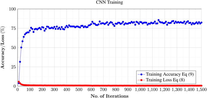
FIGURE 9. Training of the CNN using the Broadberry GPU server TYAN Thunder FT48T-B7105 with four NVIDIA GTX 1080 Ti graphics cards. The entire data set comprises of approx. 500 K images classified under 500 categories (including drone images from the augmented data library), and the entire process took approximately a week to complete the training. The blue line shows a plot training accuracy against number of iterations. The training accuracy stabilized around 80% at the end of process (approx. 1,500 iterations).

To speed up the operation of training, we had to look at batch normalization parameters; for example, where we had a batch normalization operation followed by a convolution. Note that, all the parameters for the batch normalization are constant. These constant parameters can be folded in the convolution operation. At the training stage, the batch normalization (BN) finds parameters γ (standard deviation) and β (mean) in order to regularize the variance to 1 and the average to 0 for each mini-batch. B = is our mini-batch, σ is the mini-batch variance, and x = input. The batch normalization BN algorithm for training is shown as follows:

${\mu }_B=\frac{1}{m}\sum _{i=1}^m{x}_i,(10)$

${\sigma }_B^2=\frac{1}{m}\sum _{i=1}^m{\left(x_i-{\mu }_B\right)}^2,(11)$

$BN=\gamma \frac{x-{\mu }_B}{\sqrt{{\sigma }_B^2+ϵ}}+\beta .(12)$

A hyperparameter ϵ is set for coefficient stabilization, which is used to adjust the training time. Since both γ and β have been already trained during classification, the BN can read them directly from the dynamic random access memory (DRAM). The end result of this were hundreds of megabytes of floating-point numbers, so the next step was to look at optimization (weight compression) using quantization, as the training set data needs to be loaded on the FPGA BRAM.

7 FPGA Considerations

The main advantage of FPGAs over CPUs and GPUs is that the whole system can be implemented on the same silicon, including the connections to the sensors, which reduces latency. We also have the flexibility to add new CNN layers.

Both Xilinx (Model Zoo) and Mathworks (MATLAB) provide intellectual property (IP) blocks, called deep learning processor units (DPUs). Both DPUs (from MATLAB and Xilinx) are similar hardware IPs; however, the main difference between the two DPUs is that the MATLAB DPU supports MATLAB tools, while the Xilinx DPU supports CAFFE and Tensor flow tools. Biggest advantage of these ready-made DPUs is that one can download various types of network designs. However, the downside to a DPU is that they are aimed at higher end FPGAs (such as UltraScale and UltraScale+); in other words, they are not optimized to run on a lower cost FPGA with fewer hardware resources (such as DSP slices) and are much higher power consumers. Hence, there is a greater need to design a more customized DPU that can be made portable, enabling us to run on a lower cost FPGA and using lower power consumption. Furthermore, for commercial products, the DPU IPs also comes with licensing restrictions, which make them costlier to implement and run.

Floating-point implementation on an FPGA needs the use of digital signal processing/processor (DSP) slices, which are a limited resource. Traditional CNN implementation on Xilinx Zynq FPGA requires heavy DSP48E2 slice usage for floating-point maths for each perception algorithm neuron. To solve this challenge, we needed a novel method of reducing the floating-point dependence. From our experiments, we have found that the CNN can cope with the small changes in the weights and biases of the neurons/perceptions in our network, resulting from the quantization of the floating-point values. By using quantization, we were able to reduce the weights from 32-bit floating point to 8-bit word length, which further reduced the weight memory and computation time significantly.

By using the Xilinx’s Advanced eXtensible Interface (AXI), we moved memory from valuable BRAM to external DRAM. As with the accelerated architecture used in DPUs (Zhang et al., 2020), we processed a single CNN layer at a time (i.e., in a one clock cycle) with partitioning through tiling. A block diagram of DPU engine from Xilinx is shown in Figure 10. With DPUs the PE come under the computing engine, which communicates to the inputs/weights and output buffers (stored in BRAM). In our implementation, because the network is hardcoded, we do not have the need for APB, controller, and microcode sections, leading to superior performance but reducing our flexibility, that is, we cannot process a network of a different design as ours is a fixed design.

FIGURE 10

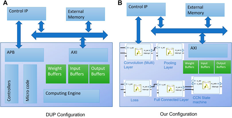
FIGURE 10. (A) Block diagram of DPU architecture from Xilinx. (B) Our implementation. Note that, we do not have application processing block (APB), controller, and microcode block (used for downloading and executing different CNN designs), instead our implementation is hardcoded to our proposed CNN network architecture.

7.1 BRAM Usage and Software Considerations on the ARM Core (PS)

With FPGAs, BRAM is required for performance but is a limited resource. BRAM uses a single clock cycle at 220 MHz, whereas as DRAM requires multiple clock cycles. The UltraScale devices have a new memory block, which provides a 6 × increase compared to BRAM. This can be enabled on the Xilinx DPU, but for our design, we have only used standard BRAM configured as 18 Kb RAM. The reason for this is make the code portable for running on non-UltraScale FPGAs. The convolution, pooling, and ReLU layers have been implemented in BRAM and grouped together on the PL. This not only increased the complexity but also improved performance, as parallel tasks can be performed in a single clock cycle. In our model, this resulted in only a third of the memory being transferred to DRAM.

For efficient CNN acceleration on FPGAs, the first task was to convert all floating operations to fixed points (Reiter et al., 2020) (Wei et al., 2019). The biggest challenge in order to complete this conversion is selecting the exponent value. We selected different exponent values for each layer, saving BRAM and other resources. For the selection, we looked at the errors of quantization per layer and channel, against the available resources. Prior to implementing the design on an FPGA, we used the MATLAB quantization tool in order to balance the amount of quantization between performance and accuracy. To do this, we used a set of images for calibration, and then we ran these though our CNN. The quantization dynamic range of the weights and biases are shown as a histogram in Figure 11. The grey shaded areas on the histogram plot (Figure 11) are the layers where quantization is not possible, and blue shaded areas are those layers where quantization is possible. We can then use our data set to estimate the reduction of the size of the network and accuracy, compared with the original network. From the results obtained for our network, we were able to achieve a reduction of approximately 73% in the size of the data set while still maintaining high accuracy.

FIGURE 11

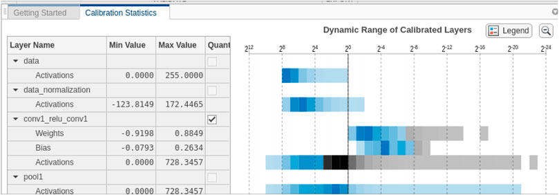
FIGURE 11. MATLAB quantization tool used to assign a scaled INT8 type for weights, biases, and activations of the convolution layers of the network, as shown in the heat map before. Gray regions of the histogram show the bits that cannot be represented. A good result is where the map is mostly blue before the black dividing line.

In our design, in order to optimize hardware resources on the PL section and when it did not affect system performance, our algorithm moved some layers to the Zynq’s Advanced RISC Machines (ARM) PS core. One such example is the “concatenation of layers” process that merges two or more layers at the channel axis. Moving this process to the PS core will not have any effect on the overall efficiency for the PS as in this case; parallel performance is not required.

7.2 FPGA Quantization Implementation Techniques to Reduce DSP Slices

For each layer output, weight, bias, and fixed-point exponent, we simply looped through each point and selected the value with the lowest quantization error. With reduction, the lower values are set to zero. The quantization is the mean square error of the real value and the quantized value. This is where we can compare the Xilinx’s Int8 format against other formats, such as FP32 as used by tensor flow (Yao et al., 2017). The INT8 technique works on the FPGA by shifting the values 18-bits to the left using the INT8 optimization. Each of the DSP slices result in a partial and independent portion of our final output values. The accumulator for each of the DSP slices is set to 48-bits. These are then chained to the next slice. This has the effect of limiting the number of chained blocks to seven, before saturation of the shifted number affects the calculation. In our implementation, each layer of the CNN has hundreds to thousands of input samples. Unfortunately, with this method, after seven terms of accumulation, the lower terms of the 48-bit accumulator might become saturated, requiring an extra DSP48E2 slice for the summation, every seven terms. This equates to 14 MACCs with every seven DSP slices plus one DSP slice for preventing saturation. This reduction in the limited DSP48E2 MACC resources requirement allows us to run this implementation on a Xilinx’s Zynq UltraScale XCZU9EG FPGA (depending on the final size of our CNN).

7.3 IP Block Integration for the Trained CNN Implementation

Our IP Block for the CNN implementation has been integrated into the block diagram, under Xilinx’s Vivado (Crockett and Northcote, 2019), with the Zynq ARM processor and the Xilinx Video Processing SubSystem (VPSS) Intellectual Property (IP) core for the camera color balance and gamma image correction. We in turn run Peta Linux, and Python. Our CNN implementation was written in HLS, a C like language, which converts the code in to PL, giving us maximum FPGA performance, while using a slow clock rate (Skliarova and Sklyarov, 2019). Unlike micro-controllers, FPGAs can run logic operations in parallel. The Xilinx Zynq ARM micro-controller is used to run the Peta Linux. This allows us to run Python script, which provides an application programming interface (API) interface between our IP Block and OpenCV graphic functions. The background-differencing algorithm is also an IP Block, running on the FPGA PL fabric and written in Verilog/VHDL, whereas the tracking code is written in Python, giving us added flexibility where top performance is not required. Graphic processing is performed using the Xilinx’s “Vitis vision” OpenCV (Johansson, 2015). For example, drawing the on-screen boxes around the detected object and displaying the on-screen object confidence weight value. OpenCV library functions are seen as essential for developing computer vision applications. The Xilinx’s “Vitis vision” libraries for computer vision, is based on key OpenCV functions, allowing us to compose and accelerate vision functions in the PL FPGA fabric. In addition, “Vitis vision” functions are consistent with OpenCV and are optimized for FPGA performance, resource utilization.

The total power consumption for our design is approximately 5.5 W. Within this total power consumption of the chip, the PL power consumption is approximately 1.2W, PS is approximately 2.65 W and the BRAM consumed 0.555 W. It should be noted that 8.1 W is the maximum for the UltraScale XCZU9EG. In Table 1, we have also compared the power consumption of our design with the MATLAB and Xilinx DPUs and our design is approximately 10–15% more efficient than the state of the art.

TABLE 1

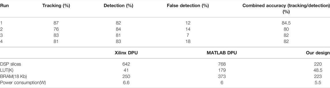
TABLE 1. Results for tracking and detection accuracy obtained in real time for four live runs. Each live run was approximately 15 min of flight time (limited by battery life). The maximum flight distance was approximately 100 m during each run. Combined accuracy is the average of tracking and detection accuracy.

8 Experimental Results

The fully integrated system contains both the detection and the tracking modules. We used our own UAV data set to evaluate the performance of the fully integrated system. The results in Table 1 is from 4 runs, at different locations, taken in real-time using real UAVs and compared against results taken from a study of human UAV operator observations (Alaparthy et al., 2021), giving better detection rate of 92%, but for periods less than half an hour versus the 24 h running of our system.

The system is designed to work in real-time, so the detection has to work at full video frame rate. Figure 12 shows the average of all the test runs taken of live tracking of UAVs against time in minutes. We recorded the weighting reported against a UAV detection and the tracking algorithm. The results show that both the tracking and CNN give good detection when the UAV is clearly visible. Once the UAV becomes around 10 or less pixels in size, both the tracking and CNN struggle. The author believes that this could be improved upon, with a zoom camera, although this could affect the tracking performance. The results also show that the combination of both the tracking and CNN produce the most accurate results for a positive identification. It also shows that tracking can continue even though not every frame has been reported as a positive UAV detection from the CNN, as the UAV still remains locked.

FIGURE 12

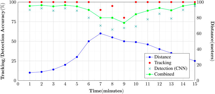
FIGURE 12. Chart showing our results for a typical detection of UAVs over a period of 15 min. As evident from the plot, nearer objects have greater tracking/detection accuracy and vice versa.

8.1 Results Comparison

We compared the MATLAB and Xilinx DPU implementation on the UltraScale ZCU102 against our model, using the same data set of images (Figure 13). We tested the performance against two network designs, AlexNet and Resnet18 which are seen as comparable against our network architecture. The frame rate is from time of receiving the image from the camera, to displaying the output results. Because of the larger size of the DPU and its requirement for more BRAM, we implemented this on the UltraScale ZCU102 development board, together with our research model. This board does not have a HDMI input, so we used the Analog devices reference design of the FMC-IMAGEON (based on the ADV7611) for both video in and out. For direct camera input, the FMC-IMAGEON interfaces to the AES-CAM-ON-P1300C-G (PYTHON-1300 color image sensor camera module). For the Xilinx DPU, we used a USB camera as supported by the Xilinx’s Vitis-AI Model Zoo Xilinx (2022) example application (using the Xilinx DPU). Only our model included the UAV tracking in the results. The video processing and NN DPU are running completely on the PL logic for the MATLAB DPU and our model. Xilinx used the Linux for camera interfacing, which adds to the latency, compare to using a direct FMC connected camera. The clock frequency of the DPU processors and our model was set at 220MHz, to give lower power consumption. The DPUs and our model all ran as a single thread and as a single core. The Xilinx DPU ran 3 cores, tripling the throughput, so the result has been adjusted accordingly. We acknowledge that performance can be greatly improved by using a higher clock rate and multiple threads/cores for each implementation, but this must be balanced against the power consumption and the maximum frame rate of the camera. The results are accessed by the ARM PS core, by reading from the DRAM for all implementations. On our CNN with tracking, we are able to achieve a high detection rate of 82% at a frame rate of 54.67 frames per second (fps). Figure 13 shows the comparison of our implementation with the nearest comparable known systems implemented using DPU engines. The Xilinx DPU actually had the highest frame rate of 184.9 fps, but this was using three cores at 224 × 224 as mentioned, so adjusting for a comparable single core system and frame size, we actually get 61.6 fps, minus the latency is then this is actually about 45 fps. As can be seen, our implementation far exceeds both in detection accuracy for UAV detection, with a higher frame rate when comparing like for like. Moreover, the CNN detection rate and the tracking rate should ideally be matched (Newcombe 2012), which is true in our case. The good performance of our model is in part due to our network design being optimized for our UAV data set with reduced number of layers as compared to Resnet18’s 18 layer structure. On the MATLAB DPU each layer takes an average of 1.8 ms, thus reducing the throughput performance for unoptimized systems. Moreover, Res18Single (single precision) achieves only 5 frames a second (as compared to 55.67 fps for ours), since it is not quantized as compared to our system, although detecting performance is slightly increased. This demonstrates the importance of quantization when implementing a CNN on an FPGA, for performance and reduced resource utilization. Our system could improve the end-to-end latency further by moving all the OpenCV video processing to the FPGA’s PL fabric, but this adds to the complexity of design and will be explored in future implementations.

FIGURE 13

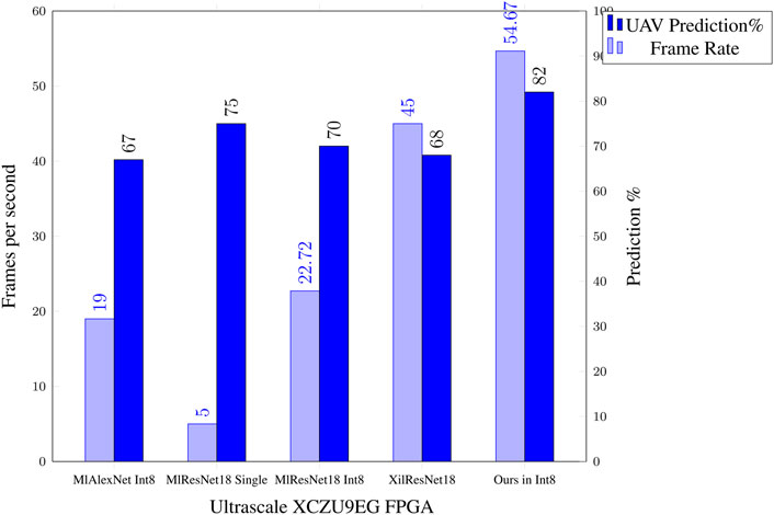
FIGURE 13. Comparison results of our FPGA CNN against a DPU MATLAB implementation (nearest known equivalent).

FIGURE 14

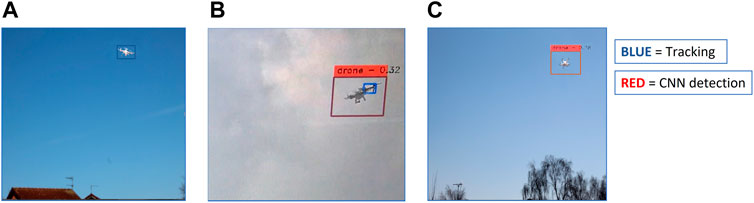
FIGURE 14. Screenshots obtained from a live system demonstrating tracking and detection of a drone during flight. The red box highlights CNN UAV detection, with weighting. The blue box highlights tracking. The panel (A) shows tracking only, while (B,C) demonstrate both tracking and CNN detection. It can be noted that (A,C) show a rooftop/trees as a point of reference, while (B) is a sky-only view. This is because the camera is continuously moving and panning in alignment with the tracking.

9 Conclusion

In this work, we have presented a novel video-based UAV monitoring system using the UltraScale XCZU9EG FPGA platform that overcomes the challenge of floating-point dependency. The system comprises the UAV detection module and the UAV tracking module. The detection module design is based on a novel CNN implementation running on FPGA’s PL fabric, together with a tracking module using novel background-differencing technique to locate UAV-shaped moving objects. We also developed model-based data augmentation technique to enrich the training data. Furthermore, we dramatically reduced the size of the training set by 73%, thus saving valuable BRAM. The fully integrated monitoring system takes advantage of both the tracking module and the CNN detector to achieve high performance monitoring. Extensive experiments were conducted to demonstrate the superior performance of the proposed UAV monitoring system. This included live real-time testing, with real radio-controlled UAVs as shown in Figure 4. Our design has shown to operate at full video frame rate with real-time processing performance thanks to FPGA’s ability to process data in parallel, just like the human brain. Our proposed implementation achieves far greater detection accuracy at considerably higher frame rates, than any other UAV tracking and detection CNN-based implementation methods, currently known.

Data Availability Statement

Requests for raw data supporting the conclusion of this article requires permission from the authors and PhD sponsor.

Author Contributions

PH carried out the research and wrote the manuscript. SS and EN verified the research and reviewed the journal manuscript, for submission.

Funding

Teledyne Lincoln Microwave is the first author’s sponsor for the PhD research at University of Lincoln.

Conflict of Interest

The authors declare that the research was conducted in the absence of any commercial or financial relationships that could be construed as a potential conflict of interest.

Publisher’s Note

All claims expressed in this article are solely those of the authors and do not necessarily represent those of their affiliated organizations, or those of the publisher, the editors, and the reviewers. Any product that may be evaluated in this article, or claim that may be made by its manufacturer, is not guaranteed or endorsed by the publisher.

Acknowledgments

The authors would like to thank Jacob Corr (University of Lincoln) for his help in training the CNN.

References

Alaparthy, V., Mandal, S., and Cummings, M. (2021). Principles of Neurodynamics. IEEE, 1–7.

Google Scholar

Baans, O. S., and Jambek, A. B. (2019). Implementation of an ARM-Based System Using a Xilinx ZYNQ SoC. Ijeecs 13, 485. doi:10.11591/ijeecs.v13.i2.pp485-491

CrossRef Full Text | Google Scholar

Chan, A. B., Mahadevan, V., and Vasconcelos, N. (2011). Generalized Stauffer-Grimson Background Subtraction for Dynamic Scenes. Mach. Vis. Appl. 22, 751–766. doi:10.1007/s00138-010-0262-3

CrossRef Full Text | Google Scholar

Chen, Y., Aggarwal, P., Choi, J., Kuo, C.-C. J., and Dec, (2017). “A Deep Learning Approach to Drone Monitoring,” in Asia-Pacific Signal and Information Processing Association Annual Summit and Conference (APSIPA ASC) (IEEE), 686–691. doi:10.1109/APSIPA.2017.8282120

CrossRef Full Text | Google Scholar

Chollet, F. (2018). Deep Learning with Python). Shelter Island, NY: Manning.

Google Scholar

Crockett, L., and Northcote, D. (2019). Exploring Zynq Mpsoc with PYNQ and Machine Learning Applications. 1 edn. University of Strathclyde.

Google Scholar

Das, S. (2020). Cnn architectures alex net, le net, vgg, google net, res net. Int. J. recent Technol. Eng. 8, 953–960. doi:10.35940/ijrte.F9532.038620

CrossRef Full Text | Google Scholar

Hanif, M., and Putra, (2018). Mpna: A Massively-Parallel Neural Array Accelerator with Dataflow Optimization for Convolutional Neural Networks.

Google Scholar

Huttunen, M. (2019). Civil Unmanned Aircraft Systems and Security: The European Approach. J. Transp. Secur 12, 83–101. doi:10.1007/s12198-019-00203-0

CrossRef Full Text | Google Scholar

Johansson, H. (2015). Evaluating Vivado High-Level Synthesis on Opencv Functions for the Zynq-7000 Fpga.

Google Scholar

Kher, H. R., and Thakar, V. K. (2014). “Scale Invariant Feature Transform Based Image Matching and Registration,” in 2014 Fifth International Conference on Signal and Image Processing, 50–55. ID 1. doi:10.1109/icsip.2014.12

CrossRef Full Text | Google Scholar

Lecun, Y., Bottou, L., Bengio, Y., and Haffner, P. (1998). Gradient-based Learning Applied to Document Recognition. Proc. IEEE 86, 2278–2324. doi:10.1109/5.726791

CrossRef Full Text | Google Scholar

Lee, S., Bang, M., Jung, K-H., and Yi, K. (2015). “An Efficient Selection of Hog Feature for Svm Classification of Vehicle,” in 2015 International Symposium on Consumer Electronics (ISCE), 1–2. ID 1. doi:10.1109/isce.2015.7177766

CrossRef Full Text | Google Scholar

Mengxi, L., Yongfeng, J., Jiuxu, S., and Zheng, W. (2018). Research of Image Recognition and Classification Based on Nin Model. J. Phys. Conf. Ser. 1098, 12031. doi:10.1088/1742-6596/1098/1/012031

CrossRef Full Text | Google Scholar

Newcombe, H. (2012). Real Time Camera Tracking when Is High Frame Rate Best. Berlin, Heidelberg: Springer Berlin Heidelberg, 222–235.

Google Scholar

Paluszek, M., and Thomas, S. (2020). Practical MATLAB Deep Learning. Berkeley, CA: Apress L. P.

Google Scholar

Reiter, P., Karagiannakis, P., Ireland, M., Greenland, S., and Crockett, L. (2020). Fpga Acceleration of a Quantized Neural Network for Remote Sensed Cloud Detection.

Google Scholar

Rosenblatt, F. (1962). Principles of Neurodynamics. Washington, DC: Spartan Books.

Google Scholar

Russakovsky, O., Deng, J., Su, H., Krause, J., Satheesh, S., Ma, S., et al. (2015). Imagenet Large Scale Visual Recognition Challenge. Int. J. Comput. Vis. 115, 211–252. doi:10.1007/s11263-015-0816-y

CrossRef Full Text | Google Scholar

Saqib, M., Khan, S. D., Sharma, N., Blumenstein, M., and Aug, (2017). “A Study on Detecting Drones Using Deep Convolutional Neural Networks,” in 2017 14th IEEE International Conference on Advanced Video and Signal Based Surveillance (AVSS) (IEEE), 1–5.

CrossRef Full Text | Google Scholar

Skliarova, I., and Sklyarov, V. (2019). FPGA BASED Hardware Accelerators, 566. Cham: Springer International Publishing AG.

Google Scholar

Wei, X., Liu, W., Chen, L., Ma, L., Chen, H., and Zhuang, Y. (2019). FPGA-based Hybrid-type Implementation of Quantized Neural Networks for Remote Sensing Applications. Sensors 19, 924. doi:10.3390/s19040924

PubMed Abstract | CrossRef Full Text | Google Scholar

Xilinx (2022). Vitis-ai-model-zoo Dpu.

Google Scholar

Yao, F., Wu, E., Sirasao, A., Attia, S., Khan, K., and Wittig, R., (2017). Deep Learning with Int8. Embedded Vision Edge Ai Vision.

Google Scholar

Zhang, X., Ye, H., Wang, J., Lin, Y., Xiong, J., Hwu, W.-M., et al. (2020). “Dnnexplorer: A Framework for Modeling and Exploring a Novel Paradigm of Fpga-Based Dnn Accelerator (Association on Computer Machinery),” in Proceedings of the 39th International Conference on Computer-Aided Design, 1–9. doi:10.1145/3400302.3415609

CrossRef Full Text | Google Scholar