Evaluation of State and Bias Estimates for Assimilation of SMOS Retrievals Into Conceptual Rainfall-Runoff Models

For an accurate estimation of land surface state variables through remote sensing data assimilation, it is important to estimate the forecast and observation biases as well. This study focuses on the evaluation of a methodology to estimate land surface state variables, together with model forecast and observation biases. Two conceptual rainfall-runoff models (HBV and GRKAL) are used for this purpose. Soil moisture data, retrieved by the Soil Moisture Ocean Salinity (SMOS) mission, are assimilated into these models for 59 unregulated sub-basins of the Murray-Darling basin in Australia. When both models simulate similar soil moisture values, the methodology results in similar forecast and observation bias estimates for both models. The same behavior is obtained when the temporal evolution of the soil moisture simulations is different, but with a similar long-term mean climatology. However, when the long-term mean climatology of both models is different, but with a similar temporal evolution, the bias estimates from both models have a different climatology as well, but with a high temporal correlation. The overall conclusion from this paper is that observation bias estimation is of key importance when updating internal state variables in a conceptual rainfall-runoff system that is calibrated to produce realistic discharge output for possibly biased internal state variables, and that the relative partitioning of bias into forecast and observation bias remains a model-dependent challenge.

1. Introduction

Soil moisture is a key variable in the hydrologic cycle, through its crucial role in the partitioning of the available radiation into latent and sensible heat fluxes, and the partitioning of rainfall into surface runoff and infiltration. Through these mechanisms, forecasted precipitation is highly sensitive to the land surface wetness conditions (Betts et al., 1996). Given the importance of soil moisture, the hydrological community has devoted significant efforts to the estimation of the surface soil moisture state at large spatial scales, and has identified a number of microwave missions that can be used for soil moisture estimation. Recent examples are the Sentinel-1 (Attema et al., 2007), the Advanced Scatterometer (ASCAT) (Figa-Saldana et al., 2002), the Soil Moisture Ocean Salinity (SMOS) (Kerr et al., 2010), the Soil Moisture Active Passive (SMAP) (Entekhabi et al., 2010), and the Global Change Observation Mission (GCOM) (Imaoka et al., 2010) missions. The major drawback of satellite soil moisture retrievals is the relatively large interval between overpasses, which can vary from a few days to multiple weeks (Li et al., 2016). The large spatial scale makes the use of these products for watershed management problematic. Furthermore, because of observation noise and errors in the inversion algorithm, remotely sensed soil moisture values will always be prone to a certain level of error. For these reasons, it has been suggested that the best way to estimate soil moisture values is the merging of satellite remote sensing and hydrologic modeling (Kostov and Jackson, 1993), which is commonly referred to as soil moisture data assimilation. Since the pilot study of Entekhabi et al. (1994), a large number of studies have put soil moisture data assimilation into practice.

Over the last few years, a number of studies have focused on the assimilation of SMOS data into hydrologic models. These studies can be classified into studies that focused on SMOS soil moisture data assimilation with the objective to obtain improved soil moisture values (Brocca et al., 2013; Dumedah and Walker, 2014b; Dumedah et al., 2014, 2015; Ridler et al., 2014; Zhao et al., 2014; Xu et al., 2015; Blankenship et al., 2016), soil moisture assimilation to improve discharge predictions (Wanders et al., 2014; Alvarez-Garreton et al., 2015; Lievens et al., 2015b), crop yields (Chakrabart et al., 2015), evapotranspiration estimates (Martens et al., 2015), atmospheric CO₂ simulations (Scholze et al., 2016), and model parameters (Dumedah and Walker, 2014a; Han et al., 2014; Lee et al., 2014). Furthermore, other studies have focused on brightness temperature assimilation (De Lannoy and Reichle, 2016b), and a comparison of brightness temperature to soil moisture assimilation (De Lannoy and Reichle, 2016a; Lievens et al., 2016). One of the outstanding issues with the assimilation of SMOS data into hydrologic models is the partitioning of biases into forecast and observation biases (Kornelsen et al., 2016).

The question of how to best deal with the bias between model forecasts and satellite observations has received significant attention. One practical approach consists of rescaling the observations so their distribution matches the distribution of the model state variables, a method commonly referred to as Cumulative Distribution Function (CDF)-matching. This was first introduced by Reichle and Koster (2004). A number of problems have been found with this approach. First, as demonstrated by Kumar et al. (2015), this approach could lead to the exclusion of unmodeled processes in the analysis results. Further, Pauwels and De Lannoy (2015) showed that CDF-matching removes the bias between observations and forecasts, but it does not correct the absolute value of the analyses or forecasts. The logical consequence is that CDF-matching may not be sufficient for coupled models, when the prediction of e.g., discharge depends on the absolute value of a model variable. Finally, a historical time series is not always available at the beginning of a new mission and data reprocessing or updates to the retrieval algorithm requires an update to the CDF-matching.

A second approach consists of a separate estimation of the model state variables and the forecast bias through the assimilation algorithm, which was first suggested by Friedland (1969). A number of studies have since then focused on separate state and forecast bias estimation, either through the inclusion of the forecast bias in the state vector (state augmentation) (Drécourt et al., 2006; Kollat et al., 2011) or the use of a dual filter (Dee and Da Silva, 1998; Dee and Todling, 2000; Dee, 2005; De Lannoy et al., 2007). Both state augmentation and the dual filter approach were compared by Drécourt et al. (2006), leading to the conclusion that both approaches lead to better model performance than when the bias is not taken into account. A number of studies have also attempted to estimate observation biases and the model state variables through the assimilation algorithm (Derber and Wu, 1998; Auligné et al., 2007; Dee and Uppsala, 2009; Montzka et al., 2013; Draper et al., 2015). Pauwels et al. (2013) developed a framework to estimate both observation and forecast biases, in addition to the model state variables, using the ensemble Kalman filter.

The question of how to best deal with biases between the model state variables and the observations for the assimilation of SMOS retrieval data remains unanswered. Most studies focusing on SMOS retrieval data assimilation removed bias through rescaling of the observations. Lievens et al. (2015b) compared a number of prior rescaling methods, and concluded that only matching the first moment of the soil moisture led to the strongest improvement in the modeled discharge. The objective of this study is to assess the results of a dual bias and state estimation algorithm for two different conceptual rainfall-runoff models. The study focuses on one-dimensional soil moisture data assimilation, using SMOS data from 2010 to 2016, across all unregulated subcatchments of the Murray-Darling basin in Australia.

2. Study Site and Data Description

The study is performed on the Murray-Darling basin in Australia, which is discussed in detail in Lievens et al. (2015a). Figure 1 shows the location of the test site and the modeled sub-basins. The basin has a drainage area of ~1 million km², and has been the subject of regular flooding over the last years. It is one of the nation's most important agricultural areas, accounting for roughly 40% of Australia's food production. Generally the catchment receives low precipitation amounts, but isolated heavy rainfall events do lead to significant flooding. Rainfall amounts vary very strongly throughout the basin. For example, in 2013 the Southern areas received ~1,200 mm, while the Western parts received <200 mm. This variability in rainfall amounts, both spatially and temporally, combined with the availability of data, make this basin both an ideal and challenging test bed for this study. Daily streamflow records have been collected for 169 gauge stations, which are mainly located along the East boundary of the basin. The drainage area for the available stations ranges between 50 and 52,000 km², with an average of 3,400 km². Daily streamflow measurements are available from 2009 to 2016 from the Water Data Online project of the Bureau of Meteorology (http://www.bom.gov.au/waterdata/). Rainfall and potential evapotranspiration were available, with a spatial resolution of 0.05°, from the Bureau of Meteorology Australian Water Availability Project (AWAP, http://www.bom.gov.au/jsp/awap/).

FIGURE 1

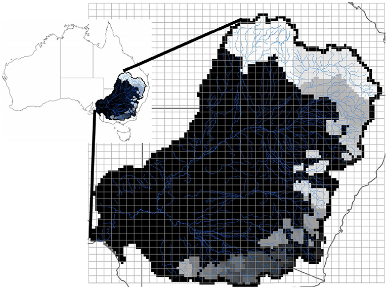
Figure 1. Location of the Murray-Darling basin in Australia. The thin lines indicate the SMOS grids. The modeled subcatchments are indicated in grayscale colors and are located in the eastern part of the basin.

The SMOS SMUDP2 v620 retrieval data were mapped onto a 36 km EASEv2 grid and conservatively screened for the impact of open water, radio frequency interference, retrieval accuracy, etc., as detailed in Koster et al. (2016). The bottom panel of Figure 1 shows the overlay of the SMOS grid on the study area.

For each subcatchment, spatially averaged soil moisture observations and meteorological forcings were used in the study. These were calculated by summing the SMOS observations (or the AWAP data) for all SMOS (or AWAP) grids located inside the subcatchment, and dividing by the number of grids inside the subcatchment.

SMOS data from June 2010 to December 2016 were used. The number of available SMOS observations varied strongly between the studied catchments. In order to draw reliable conclusions, only the catchments with at least 100 soil moisture observations throughout the simulation period were retained. Based on this criterion, the results for 59 subcatchments of the Murray Darling basin were analyzed.

3. Model Description

To study the relative effect of various biases in various rainfall-runoff models, and to check the robustness of the assimilation system, two models with a different representation of soil moisture are used in this study.

3.1. The HBV Model

One model used in this study is the Hydrologiska Byråns Vattenbalansavdelning (HBV) model, that was originally developed by Linström et al. (1997), and is described in detail in Pauwels et al. (2013). In its original formulation, the model uses observed precipitation (R_tot) and potential evapotranspiration (ETP) as input. The catchment is divided into a soil reservoir (with storage S), a slow reservoir (with storage S₁), and a fast reservoir (with storage S₂). The state vector in the assimilation procedure consists of these three variables, and for each of these variables the forecast bias is calculated. Table 1 lists the model parameters and their minimum and maximum value for the model parameter estimation.

TABLE 1

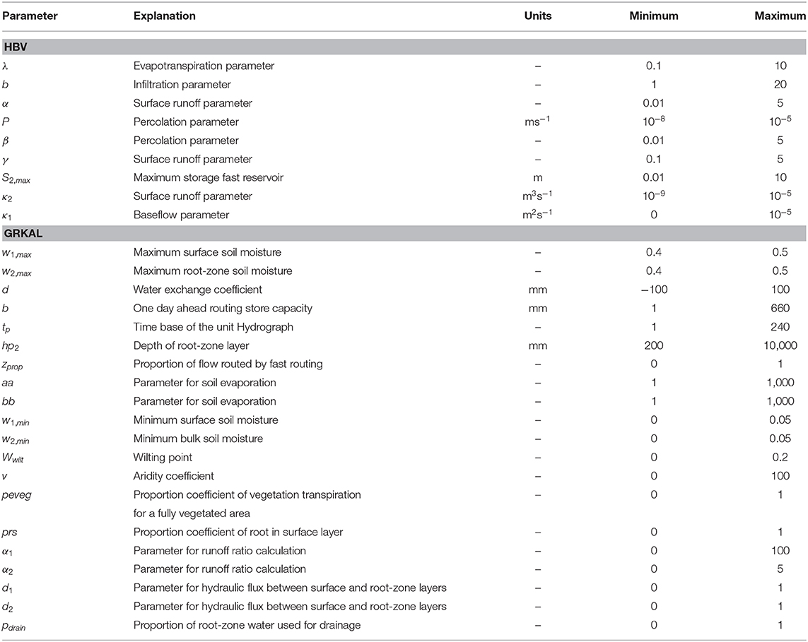
Table 1. Calibrated model parameters and their minimum and maximum values in the parameter estimation.

The modeled discharge is routed to the catchment outlet using a triangular unit hydrograph. The amount of time steps in the unit hydrograph is referred to as the base time, and the value of the unit hydrograph increases linearly from zero at time zero to the maximum at half the base time. After this, the unit hydrograph decreases linearly from the maximum value at half the base time to zero at the base time. The unit hydrograph value at half the base time is calculated so that the integral of the unit hydrograph is equal to one. The base time of the unit hydrograph is a calibrated parameter as well.

3.2. The GRKAL Model

The second model is the Génie Rural Kalman model (GRKAL), as described in Francois et al. (2003). This is based on the daily conceptual model GR4 (Loumagne et al., 1996). The rainfall is partitioned into infiltration into the soil column and a subterranean layer. The soil column consists of a thin upper layer and a deeper lower layer. The state vector in the assimilation algorithm consists of the water content of this thin layer, the deeper lower layer, and the subterranean layer. Again, for each of these storages the forecast bias is calculated. The root fraction of these two layers determines the partitioning of the evapotranspiration between the layers. Diffusive exchange of water between the two layers is modeled based on their water contents. A one-parameter baseflow formulation is used. The baseflow is then added to the subterranean layer. The overland flow is then routed to the outlet through a triangular unit hydrograph, and the baseflow is routed using a linear reservoir. The sum of the routed baseflow and surface runoff is the catchment discharge. For a detailed model description we refer to Francois et al. (2003). Table 1 lists the model parameters and their minimum and maximum value for the model parameter estimation.

4. Model Parameter Estimation

Prior to the assimilation of SMOS soil moisture retrievals, both models are calibrated to ensure that both models simulate similar, realistic, levels of discharge.

4.1. The Parameter Estimation Algorithm

The parameter estimation algorithm used in this paper, Particle Swarm Optimization, PSO (Kennedy and Eberhart, 1995), is based on the complex, collective behavior of individuals in decentralized, self-organizing systems. These systems are created through a population of individuals that interact locally with each other and with the community. These interactions lead to global behavior, which can result in the achievement of certain objectives. Examples of such systems in nature are abundant: ant colonies, swarms of birds, and schools of fish. For a complete description of the algorithm we refer to Scheerlinck et al. (2009).

4.2. Application

For each of the 59 modeled sub-basins of the Murray-Darling basin, the model was applied from January 1, 2009, to December 31, 2016, using a daily time step. The Root Mean Square Error (RMSE) between model simulations and observations of discharge (Q_o and Q_s, respectively, in m³s⁻¹) was calculated as follows:

$\begin{array}{ll}\text{RMSE}=\frac{1}{N_q}{\displaystyle \sum _{i=1}^N}{(Q_o(i)-Q_s(i))}^2& (1)\end{array}$

N_q is the amount of discharge observations. The model parameters listed in Table 1 were estimated, as well as the base time of the unit hydrograph of the HBV model.

Two different calibration strategies have been applied. First, the model was calibrated using discharge data from the entire simulation period. The results of the SMOS data assimilation algorithms will then be evaluated during the calibration period. Second, the model was calibrated using the discharge observations from 2009 to 2013. The data assimilation algorithms will then be validated using data from the validation period (2014–2016). In the second calibration strategy, SMOS data were assimilated only during 2014–2016, while in the first SMOS data from 2010 onwards were used. This strategy allowed an understanding of the robustness of the methodology, by applying the model to a time period that was used to estimate the model parameters, and a second time period that was not used in the model calibration. Unless noted otherwise, the remainder of the paper will mainly refer to the results from the first strategy.

5. Assimilation of SMOS Data

5.1. Short Description of the Assimilation Algorithm

In this study, the dual observation/forecast bias and state variable estimation algorithm described in Pauwels et al. (2013) was used. This algorithm consists of an ensemble Kalman filter, estimating the system state variables, and two discrete Kalman filters, one for the observation and forecast biases, respectively. Figure 2 shows an overview of the methodology. The biased system state vector ${\tilde{\text{x}}}_k$ is propagated as follows:

$\begin{array}{ll}{\tilde{\text{x}}}_k=f_{k,k-1}({\tilde{\text{x}}}_{k-1},{\text{u}}_k,{\text{w}}_k)& (2)\end{array}$

k is the time step, f_k,k−1 the non-linear model propagating the state from time step k − 1 to time step k, ${\tilde{\text{x}}}_k$ is the biased state vector, u_k the model forcings, and w_k the model error. For the remainder of the paper, variables indicated with a $\left[\begin{array}{c}~\\ .\end{array}\right]$ indicate biased variables, with biased a priori forecast error covariance ${\tilde{\text{P}}}^{-}$. The unbiased state vector x_k is:

$\begin{array}{ll}{\text{x}}_k={\tilde{\text{x}}}_k-{\text{b}}_k^f& (3)\end{array}$

with unbiased a priori forecast error covariance P⁻. ${\text{b}}_k^f$ is the forecast bias. The system is observed as follows:

$\begin{array}{ll}{\tilde{\text{y}}}_k={\text{H}}_k{\text{x}}_k+{\text{b}}_k^o+{\text{v}}_k& (4)\end{array}$

H_k is the observation operator (assumed linear), ${\tilde{\text{y}}}_k$ is the vector with the biased observations, and v_k the observation noise. v_k is Gaussianly distributed with mean zero and variance R_k. The unbiased observations are:

$\begin{array}{ll}{\text{y}}_k={\tilde{\text{y}}}_k-{\text{b}}_k^o& (5)\end{array}$

${\text{b}}_k^o$ is the observation bias. The forecast and observation biases are propagated as follows:

$\begin{array}{ll}\{\begin{array}{ccc}{\text{b}}_k^f& =& {\text{b}}_{k-1}^f\\ {\text{b}}_k^o& =& {\text{b}}_{k-1}^o\end{array}& (6)\end{array}$

with a priori forecast bias error covariance ${\text{P}}_k^{f-}$ and a priori observation bias error covariance ${\text{P}}_k^{o-}$. ${\text{b}}_{k-1}^f$ consists of the forecast bias estimate for the three model variables for both models, while ${\text{b}}_{k-1}^o$ consists of the estimate of the bias in the observed soil moisture. Pauwels et al. (2013) describe in detail the state and bias update equations. For these updates, the biased and unbiased background error covariances, and the observation and forecast bias error covariances are needed. The biased a priori background error covariance ${\tilde{\text{P}}}_k^{-}$ can be diagnosed from ensemble forecast integration (Reichle et al., 2002), based upon which the unbiased background error covariance ${\text{P}}_k^{-}$ and the forecast bias error covariance ${\text{P}}_k^{f-}$ can be calculated as:

$\begin{array}{ll}\{\begin{array}{lll}{\tilde{\text{P}}}_k^{-}& =& {\gamma }_f{\text{P}}_k^{-}\\ {\text{P}}_k^{f-}& =& (1-{\gamma }_f){\text{P}}_k^{-}\end{array}& (7)\end{array}$

The superscript ⁻ indicates a prior value, before the updating. γ_f is a filter parameter, between zero and one, which determines the amount of update to the state and the bias, and which can be obtained through calibration. Note that the forecast bias errors are thus assumed to be correlated in the same way as the forecast state errors, allowing an estimation of the bias in unobserved variables. The observation bias error covariance is calculated as:

$\begin{array}{ll}{\text{P}}_k^{o-}={\kappa }_o{\text{H}}_k{\tilde{\text{P}}}_k^{-}{\text{H}}_k^{\text{T}}& (8)\end{array}$

The matrix ${\text{H}}_k{\tilde{\text{P}}}_k^{-}{\text{H}}_k^{\mathrm{\text{T}}}$ is the error covariance of the observation predictions, and can be calculated in a computationally efficient way using the ensemble statistics, as described in Pauwels and De Lannoy (2009). κ_o is a filter parameter and can be estimated through calibration as well.

FIGURE 2

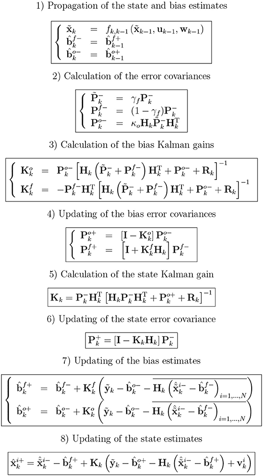
Figure 2. Schematic of the methodology of the assimilation algorithm. N is the ensemble size, and i indicates the ensemble member number.

5.2. Terminology

For the remainder of the paper, the following consistent terminology is used.

The term “biased observations” refers to SMOS soil moisture retrievals, without bias removal. On the other hand, “unbiased observations” refers to the SMOS soil moisture observations, from which the estimated observation bias has been removed. “Observation bias” is the bias in the SMOS soil moisture observations, but it can also refer to the more general bias between SMOS observations and observations predictions. In other words, the observation bias includes both soil moisture retrieval bias and representativeness bias.

For the model results, a similar terminology is used. “Biased simulations” and “biased results” refer to the modeled soil moisture (from either GRKAL or HBV), again without bias removal. “Unbiased simulations” and “unbiased results” are the soil moisture simulations, from which the estimated forecast bias has been removed. “Forecast bias” means the bias in the modeled (GRKAL or HBV) soil moisture.

“Baseline simulations” or “baseline results” refer to the model simulations without SMOS retrieval assimilation. “Assimilation run” refers to model simulations with the assimilation of SMOS soil moisture data.

In the sections below, all evaluations are based on ensemble mean forecasts and analyses.

5.3. Filter Application

The filter parameters, γ_f and κ_o, are calibrated through examining the Gaussianity of the innovations. These parameters are assumed constant throughout the entire simulation, and are determined through minimizing an objective function. More specifically, the normalized innovations for the bias and state updates need to be Gaussianly distributed. When one observation is assimilated, these requirements for the bias and state innovations can be respectively written as:

$\begin{array}{ll}\begin{array}{c}\frac{{\text{y}}_k-{\widehat{\text{b}}}_k^{o-}-\overline{{\text{H}}_k{\left({\widehat{\tilde{\text{x}}}}_k^{i-}-{\widehat{\text{b}}}_k^{f-}\right)}_{i=1,\dots ,N}}}{\sqrt{{\text{H}}_k\left({\tilde{\text{P}}}_k^{-}+{\text{P}}_k^{f-}\right){\text{H}}_k^{\text{T}}+{\text{P}}_k^{o-}+{\text{R}}_k}}~\text{N}\left(0,1\right),\\ \frac{{\text{y}}_k-{\widehat{\text{b}}}_k^{o+}-\overline{{\left({\text{H}}_k\left({\widehat{\tilde{\text{x}}}}_k^{i-}\right)\right)}_{i=1,\dots ,N}}}{\sqrt{{\text{H}}_k{\tilde{\text{P}}}_k^{-}{\text{H}}_k^{\text{T}}+{\text{P}}_k^{o+}+{\text{R}}_k}}~\text{N}\left(.,1\right)\end{array}& (9)\end{array}$

$\left[\begin{array}{c}^\\ .\end{array}\right]$ indicates an estimate of the state or bias vector, i is the ensemble member number, N is the ensemble size, and the overline refers to ensemble means. The superscript ⁺ indicates a posterior value, after the updating, and the error covariance matrices effectively collapse to scalar error variances.

Sections 3.1 and 3.2 describe the three state variables $\widehat{\tilde{\text{x}}}$. Consequently, the state and forecast bias vectors consist of three entries. Since the water content of the upper layer in each model can be directly compared to the SMOS soil moisture observations, and because only one observation is assimilated at each assimilation time step (leading to observation and observation bias vectors with one entry), the observation operator can be written as:

$\begin{array}{ll}{\text{H}}_k=\left[\begin{array}{c}1\\ 0\\ 0\end{array}\right]& (10)\end{array}$

An ensemble of 32 members was selected for the study, to dynamically estimate ${\tilde{\text{P}}}_k^{-}$ (and to derive ${\text{P}}_k^{-}$, ${\text{P}}_k^{f-}$, and ${\text{P}}_k^{o-}$, following Equations 7 and 8). Pauwels et al. (2013) and Pauwels and De Lannoy (2015) have shown that this is a sufficiently large ensemble for data assimilation studies with the HBV model. A Gaussian random number with mean zero and standard deviation of 10% of the parameter or forcing input value is added to each model parameter for the first model time step, and to each forcing variable (precipitation and potential evapotranspiration) at each time step. This is the same strategy as was applied in Pauwels and De Lannoy (2015). A lower and upper bound was set for all parameters and forcing variables, in order to avoid physically unrealistic values. For the model parameters, these bounds are the values in Table 1. For the precipitation, a lower bound of 0 was used.

6. Results

6.1. Estimation of the Model Parameter

The left hand side panel of Figure 3 shows the distribution of the Nash-Sutcliffe Efficiency (NSE) obtained using the optimal model parameter set for the 59 sub-basins of the Murray-Darling basin, for the model calibration over the entire simulation period. This efficiency is calculated as:

$\begin{array}{ll}\text{NSE}=1-\frac{\text{MSE}}{{\sigma }_o^2}& (11)\end{array}$

${\sigma }_0^2$ is the variance of the observed discharge values. MSE is the mean square error, which is the square of the value calculated in Equation (1). The average NSE for all 59 catchments is roughly similar for the two models.

FIGURE 3

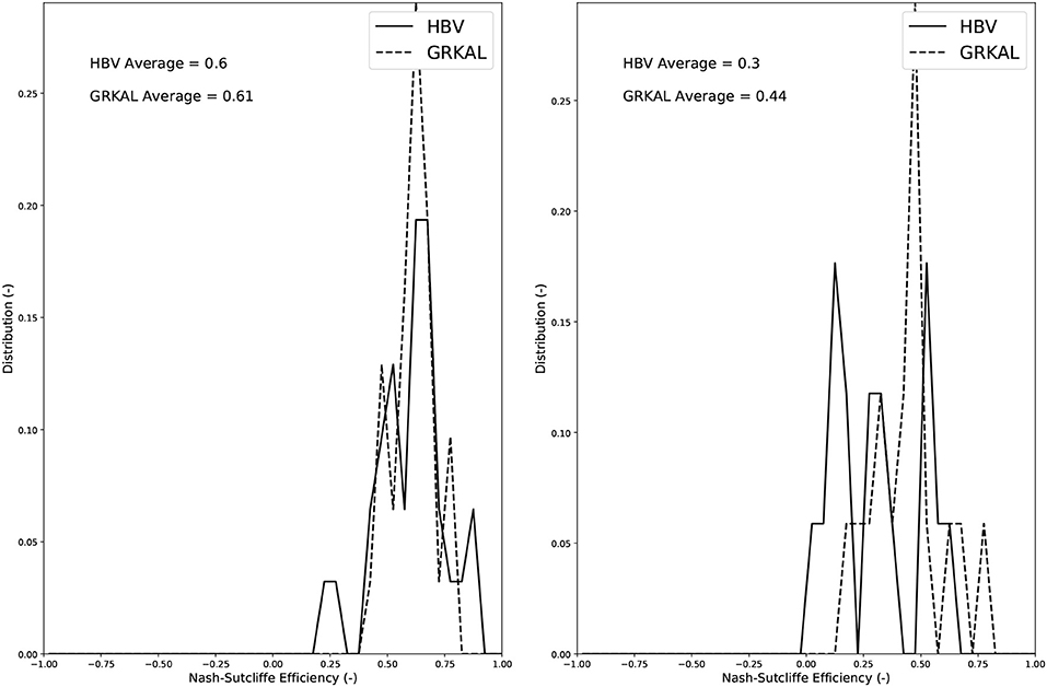
Figure 3. Distribution of the HBV and GRKAL Nash-Sutcliffe efficiencies over the 59 modeled sub-basins of the Murray-Darling basin. Left hand side panel: Results for the calibration over the entire simulation period. Right hand side panel: Results for the separate validation period (2014-2016).

Figure 4 shows the comparison of the modeled discharge to the observations for the smallest modeled catchment in the basin (401015, 781 km²), the catchment with the median drainage area in the basin (410048, 1,406 km²), and the largest catchment in the basin (422201E, 81,250 km²). The NSE values for these three catchments are within one standard deviation of the average, and can thus be considered as values typically obtained for the 59 catchments.

FIGURE 4

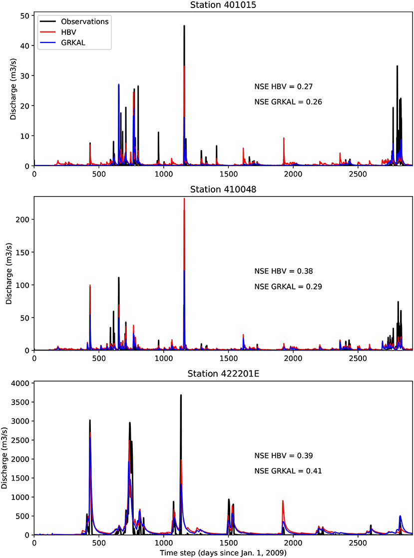
Figure 4. Comparison of the modeled to the observed discharge for the three selected sub-basins of the Murray-Darling basin.

The right hand side panel of Figure 3 shows the distribution of the Nash-Sutcliffe Efficiency (NSE), for the validation period (2014–2016), when calibrating the model using data from 2009 to 2013. As can be expected, these NSE values are lower than the results without a separate validation.

For a number of subcatchments a relatively low NSE has been obtained. This can be explained by a number of issues. First, there is the rainfall forcings, which will inevitably have a relatively large uncertainty for this very large area with a relatively coarse coverage of stations. The catchments are also characterized by extreme changes between dry and wet conditions and agricultural water management practices, which are very difficult to model. Overall, the models perform relatively well, but there are catchments where the performance is low.

The model performance can be assumed, for some catchments, to be too weak for operational flood management purposes. However, to assess the impact of soil moisture assimilation on the bias and state variable estimates of the models from a methodological point of view, these results can be assumed to be sufficiently accurate.

6.2. Estimation of the Filter Parameters

The filter parameters γ_f and κ_o were estimated in order to fulfill Equation (9). The objective function (OF) that was minimized for each river basin individually is:

$\begin{array}{ll}\text{OF}={(S_s-1)}^2+M_b^2+{(S_b-1)}^2& (12)\end{array}$

S_s is the standard deviation of the normalized state update innovations (bottom part of Equation 9), M_b the mean of the normalized bias update innovations (top part of Equation 9), and S_b the standard deviation of the normalized bias update innovations (top part of Equation 9). For γ_f, relatively consistent estimates were obtained across all basins, with an average and standard deviation of 0.051 and 0.008, respectively, for the HBV model. For the GRKAL model, the average and standard deviation were 0.05 and 0.004. However, for κ_o, more variable results were obtained. For the HBV model the average was 556.9 with a standard deviation of 421.5. For GRKAL the average and standard deviation were 33.8 and 39.7, respectively. This can be explained by the way the models simulate soil moisture. In other words, the variable soil moisture for the HBV model does not have the same physical meaning as for the GRKAL model. However, the same observation is used for both models, and it has again a different physical meaning. It can thus expected that the parameters used to estimate the observation bias will be different for both models.

This further implies that the estimated forecast bias uncertainty (~0.95/0.05 ${\tilde{\text{P}}}_k^{-}$, Equation 7) tends to be relatively much smaller than the observation uncertainty (up until ~1,000 ${\tilde{\text{P}}}_k^{-}$, Equation 8), and both are larger than the a priori forecast state error covariance. The larger spread in the observation bias errors is a strong indicator that the observation bias will be the most updated in the following results.

6.3. Analysis of the Filter Parameters

In order to analyze the impact of the filter parameters, a sensitivity analysis was performed. Figure 5 shows, for both hydrologic models, the results of a sensitivity analysis for the filter parameters for one example river basin. Similar results were obtained for all other sub-basins. More specifically, the NSE is calculated between the observation biases obtained using predefined filter parameters, and the observation biases obtained by varying filter parameters, as follows:

$\begin{array}{ll}\text{NSE}=1-\frac{{\displaystyle \sum _{i=1}^{N_b}}{(b_{v,i}-b_{c,i})}^2}{{\displaystyle \sum _{i=1}^{N_b}}{(b_{c,i}-\overline{b_c})}^2}& (13)\end{array}$

N_b is the number of time steps with bias estimates (2,182), and b_v,i and b_c,i are the bias estimates with variable and predefined filter parameters, respectively. These predefined filter parameters were assigned rather high values, more specifically 0.3 for γ_f, and 500 and 150 for κ_o for the HBV and GRKAL models, respectively. A strongly varying NSE with respect to the parameter values thus indicates a high sensitivity of the filter results to the parameter values. A similar analysis has also been performed for the forecast bias. An examination of Figure 5 leads to the conclusion that the biases are sensitive to the value of γ_f only for relatively low values of κ_o. For higher values of κ_o the obtained biases are no longer sensitive to the value of γ_f. Further, as can be expected, the forecast bias is more sensitive to the value of γ_f than the observation bias.

FIGURE 5

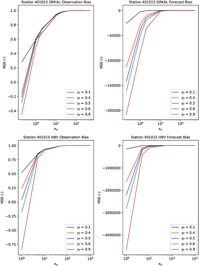
Figure 5. Left hand side panels: NSE between the observation bias obtained with γ_f 0.35 and κ_o 500 for the HBV model and κ_o 150 for the GRKAL model, and variable values for these parameters, for the first selected station. Right hand side panels: same for the forecast bias. The top panels show the results for the GRKAL model, the bottom panels for the HBV model.

Figure 6 shows the statistics of the innovations for the first selected sub-basin. Following Equation (9), the mean of the bias innovations has to be equal to zero, and the standard deviation of the state and bias innovations has to be equal to one. These optimum values are obtained for high values of κ_o. Again, similar results were obtained for the remaining sub-basins. The statistics are sensitive to the value of γ_f only for small values of κ_o. Furthermore, good innovation statistics are only obtained for relatively large values of κ_o.

FIGURE 6

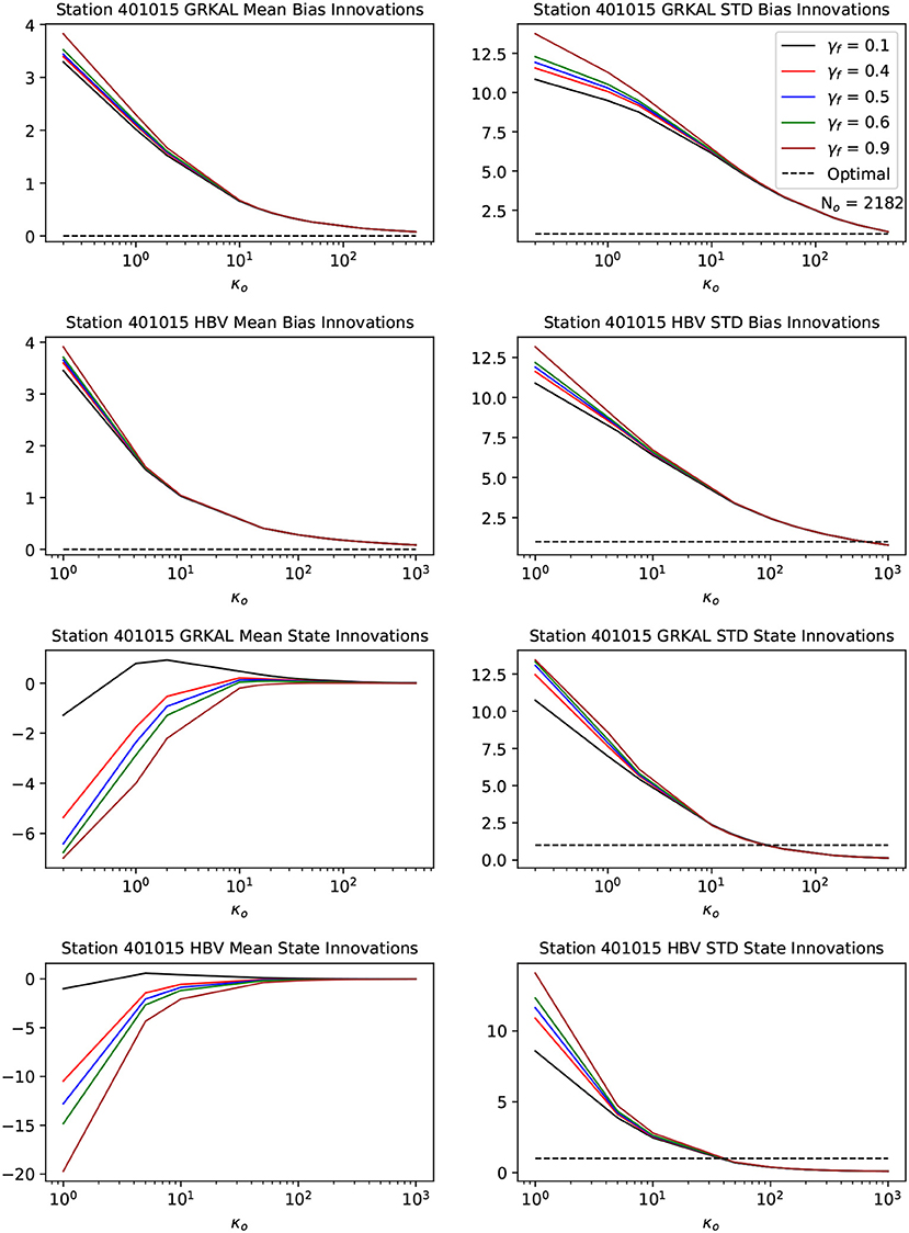
Figure 6. Statistics of the innovations obtained with variable values for γ_f and κ_o. The horizontal dashed black line indicates the optimal value. The top four panels show the bias innovation statistics, the bottom four panels the state innovation statistics. The left hand side panels show the means of the innovations, the right hand side panels the standard deviations.

6.4. Assimilation of the SMOS Soil Moisture Data

6.4.1. Analysis of the Bias Estimates for a Selected Sub-Basin

Figure 7 compares the bias and the soil moisture estimates for the second selected sub-basin for both models. The Nash-Sutcliffe Efficiency (NSE) values in the plots are calculated as follows:

$\begin{array}{ll}\text{NSE}=1-\frac{{\displaystyle \sum _{i=1}^{N_s}}{(G_i-H_i)}^2}{{\displaystyle \sum _{i=1}^{N_s}}{(H_i-\overline{H})}^2}& (14)\end{array}$

N_s is the number of time steps with soil moisture observations, and G_i and H_i are the results for the GRKAL and HBV models, respectively. The top and middle panel show the observation and forecast bias estimates, respectively. From these plots it can be seen that the observation bias estimates are an order of magnitude larger than the estimates of the forecast bias. Furthermore, there is a stronger agreement in absolute terms between the observation bias estimates for both models than between the forecast bias estimates, even though the correlations are similar. This can be expected, as the observation bias depends in the first place on the remotely sensed observations, and secondly on the models. Representativeness error, meaning that each model has a different definition of soil moisture, also contributes to the observation bias. The forecast biases for the two models are very different, as indicated by the very low NSE. This can be explained by the different soil moisture dynamics of the two models, which is demonstrated in the bottom panel of Figure 7. Even though the models show very different soil moisture estimates, the forecast bias estimates do not compensate for this large difference and the bias-corrected forecasts are very different and each approaching a different “truth.” This is because each model is calibrated to produce the right discharge with each a different soil moisture climatology. The conclusion that can be drawn from Figure 7 is that the agreement between the observation bias estimates for both models is relatively high and dominated by retrieval bias, whereas the forecast bias and modeled soil moisture estimates are strongly different.

FIGURE 7

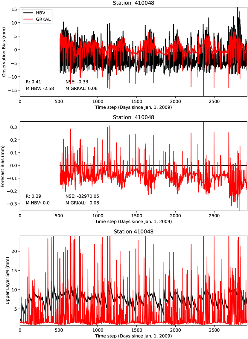
Figure 7. Comparison of the estimated observation bias (top), forecast bias (middle), and upper layer soil moisture values (bottom) for the HBV and GRKAL models, for the second selected sub-basin. M stands for mean.

6.4.2. Analysis of the Bias Estimates

For the analysis of the bias estimates, three different stations were selected. Figure 8 shows the comparison of the observation and forecast bias estimates and the upper layer soil moisture for these three selected sub-basins. It should be clarified that these soil moisture estimates were obtained from the baseline run. A first station (403241A), shows very similar upper layer soil moisture estimates for the two models. A second station, 405246A, shows a very different upper layer soil moisture climatology for the two stations, but a relatively similar temporal evolution. Finally, a third station (405269A), shows the opposite behavior: a relatively similar upper layer soil moisture climatology, but a strongly different temporal evolution. For station 403241A, the soil moisture estimates from both models are very similar. Consequently, for station 403241A the observation and forecast biases are very similar as well. For station 405246A the mean bias estimates for both models are very different, but with a relatively similar temporal evolution, which is indicated by the value of 0.61 and 0.53 for the correlation between the observation and forecast bias estimates, respectively, for both models. For station 405269A again relatively similar observation and forecast bias estimates are obtained for the two models, even though the temporal evolution of the soil moisture estimates is very different, but with relatively similar climatologies.

FIGURE 8

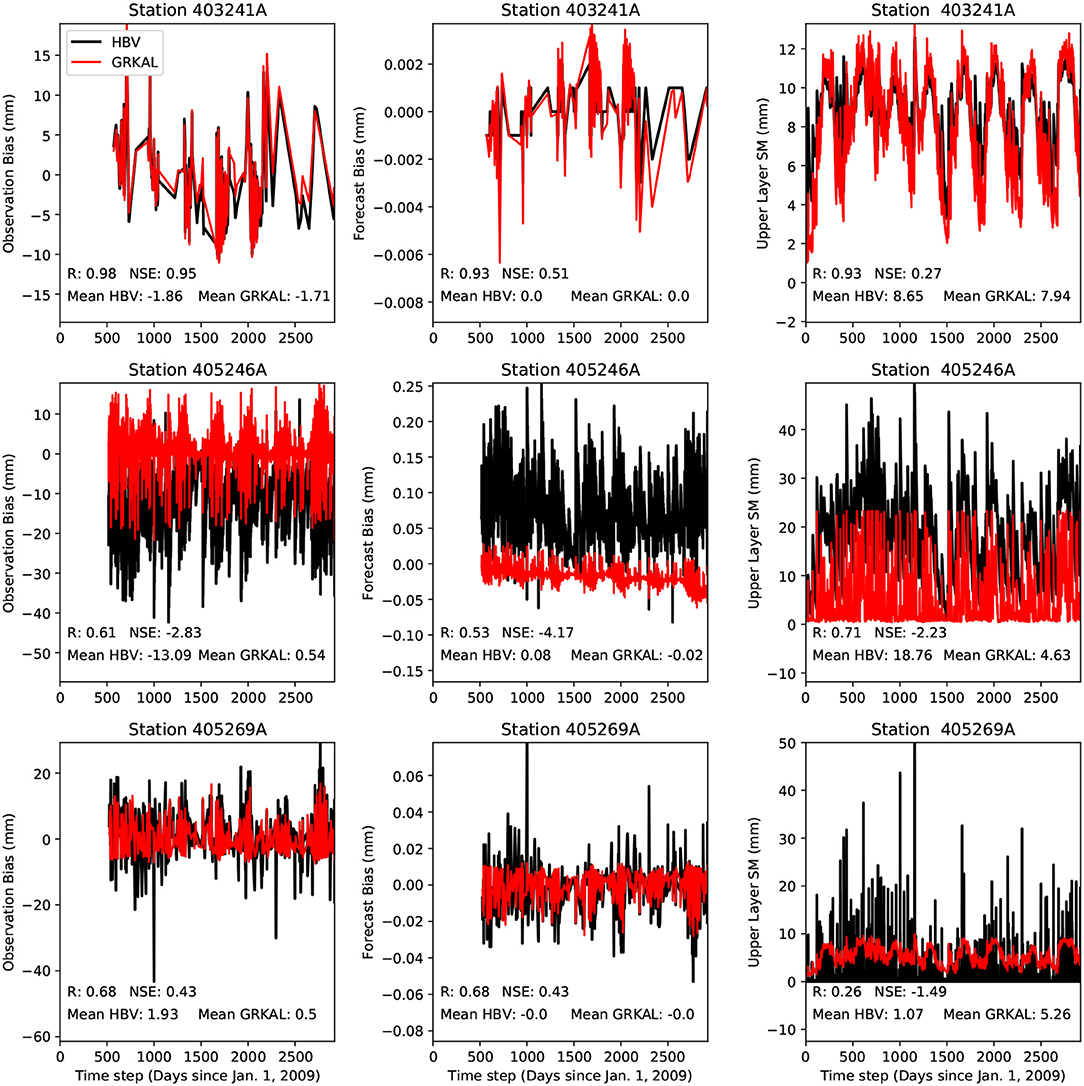
Figure 8. Comparison of the observation for forecast biases and the upper layer soil moisture estimates for three selected sub-basins.

These examples represent the three extreme cases for all the modeled sub-catchments. Either the soil moisture estimates are very similar, in which case the biases are also similar. In case the soil moisture estimates are completely different, two different behaviors of the biases can be observed. When the average soil moisture for the two models is similar, similar biases are obtained. When the means are different, different bias values result, but still with a relatively high agreement in the temporal evolution of the bias.

These results provide support to a framework in which both observation bias and model forecast bias are estimated, but the joint identifiability of both biases remains a topic to be further explored in more studies. Its feasibility can be expected to be strongly dependent on the types and amounts of available observed data.

Figure 9 shows the distribution of the NSE values, correlation coefficients, and mean average difference between the soil moisture values, and the observation and forecast biases, estimated by both models, for all modeled sub-basins. For the soil moisture values, the correlation coefficients tend to be rather high, with relatively low NSE values, indicating that the middle panel of Figure 8 is the most representative for the modeled basins. This is supported by an analysis of the observation biases, which show relatively high correlation coefficients as well, with a relatively low NSE. The forecast biases also show relatively high correlation coefficients (albeit not as high as the observation bias), with very low NSE values. This can be explained by the middle panel of Figure 7, which shows a more variable forecast error for GRKAL than for the HBV model. As the NSE is calculated as one minus the RMSE divided by the variance, this low standard deviation will lead to very low NSE values. The conclusion from Figure 9 is that the soil moisture estimates from both models, as well as the observation and forecast biases, in general show a relatively high temporal correlation. The observation bias estimates from both models are in better agreement than the forecast bias estimates.

FIGURE 9

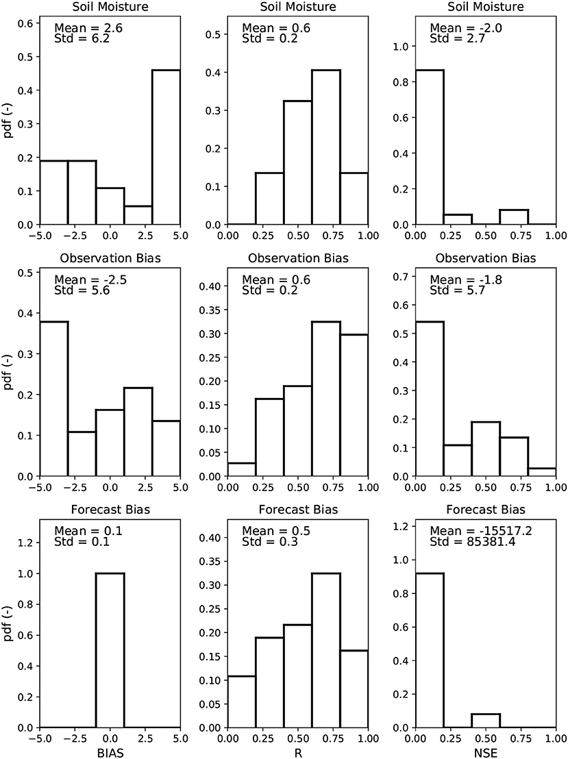
Figure 9. Distribution of the biases (left hand side column), correlation coefficients (middle column), and NSE values (right hand side column) between the results obtained by the HBV and GRKAL models, for all subcatchments. (Top) Modeled soil moisture. (Middle) Observation bias. (Bottom) Forecast bias. Results lower than the lowest values in the plot are added to the lowest class, and results higher than the highest value are added to the highest class.

Figure 10 shows the same distributions and statistics, but for the validation period for the applications with a separate calibration and validation period. Essentially the same conclusions can be drawn as for Figure 9, indicating the robustness of the methodology.

FIGURE 10

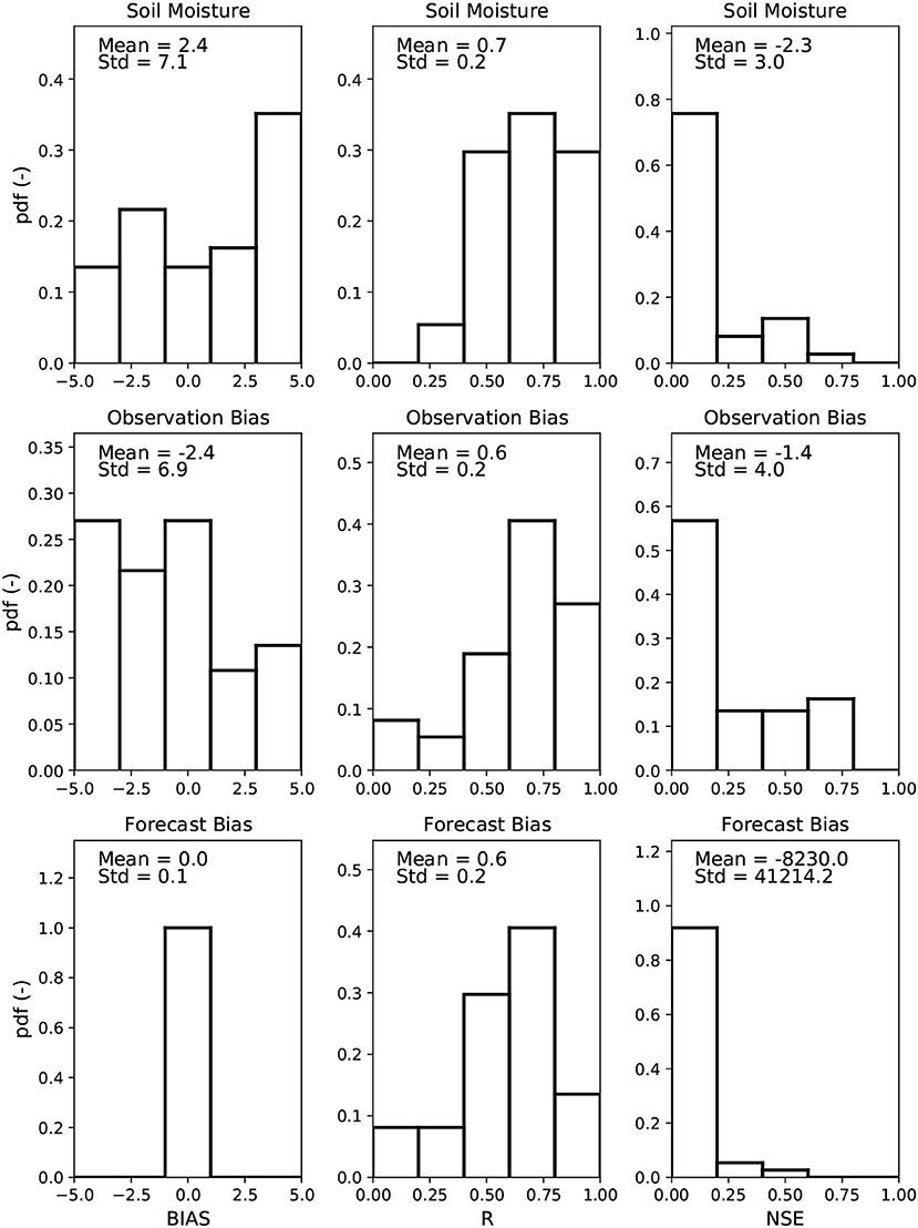
Figure 10. Same as Figure 9, but results for the validation period for the applications with a separate calibration and validation period.

6.4.3. Impact on the Discharge Forecasts

The impact of the data assimilation on the discharge forecasts has yielded mixed results. For the HBV model, the average NSE of the baseline and assimilations runs was unaltered, regardless of whether a separate calibration and validation period was used or not. In the case of separate calibration and validation periods, the data assimilation had a positive impact on the discharge estimation for 31 stations, and a negative impact for 24 stations. During the separate calibration period, a positive impact was obtained for 35 stations, and a negative impact for 19 stations. However, in both cases, the data assimilation only changed the NSE by 0.05 or less on average.

A stronger impact was found for the GRKAL model. In the case of no separate calibration and validation, the NSE between the observed and simulated discharge reduced to −1.52, with a reduction of more than 0.05 for 19 stations, and more than 0.5 for 8 stations. A positive and negative impact was obtained for 5 and 50 stations, respectively. In the separate validation period, the NSE reduced to −6.60, with a positive and negative impact for 8 and 47 stations, respectively. For 17 stations a reduction of more than 0.05 was obtained, with a reduction of more than 0.5 for 12 stations, respectively. Overall, the impact of the DA is negative for the GRKAL model, with this average negative impact being caused by a small number of strongly negatively impacted stations.

This discrepancy can be explained by the calibration of the models, which did not take into account the soil moisture content, and only focussed on optimizing the discharge forecasts. Furthermore, both models calculate the soil moisture contents in strongly different ways. In other words, they define soil moisture in different ways, not consistent with the definition of soil water content by the SMOS satellite. Despite the bias estimation, it is thus not surprising that the assimilation of external soil moisture values did not improve the discharge forecasts. The potentially negative impact of soil moisture assimilation on discharge forecasts was also noted by Mao et al. (2019).

7. Discussion and Conclusions

The objective of this paper was to evaluate a strategy to assimilate SMOS data into conceptual hydrologic models. Both the state variables and observation and forecast biases are estimated using a dual state and observation/forecast bias estimating ensemble Kalman filter. The GRKAL and HBV models were used for this purpose. When the soil moisture estimates from both models are in good agreement, the observation and forecast bias estimates are in good agreement as well. When the soil moisture estimates from both models are different, with a different climatology but a relatively high temporal correlation, the bias estimates still show a relatively high temporal correlation. On the other hand, if the soil moisture estimates have a low temporal correlation but a relatively similar climatology, the bias estimates are again relatively similar. Further research can focus on the assimilation of remote sensing data into physically-based land surface models.

Data Availability Statement

All data used in this study are publicly available and can be downloaded from the Bureau of Meteorology (BoM) Australian Water Availability Project (AWAP), http://www.bom.gov.au/jsp/awap/index.jsp.

Author Contributions

VP performed the modeling aspects of the work and wrote the paper. GD and H-JH helped in the interpretation of the results and the structuring of the manuscript.

Funding

For this study, VP was funded by ARC Future Fellow grant FT130100545.

Conflict of Interest

The authors declare that the research was conducted in the absence of any commercial or financial relationships that could be construed as a potential conflict of interest.

Acknowledgments

This work was supported by computational resources provided by the Australian Government through the National Computational Infrastructure under the National Computational Merit Allocation Scheme. We also thank the Bureau of Meteorology for the discharge, rainfall, and evapotranspiration data. We express our gratitude to Dr. Stefania Grimaldi for making Figure 1.

References

Alvarez-Garreton, C., Ryu, D., Western, A. W., Su, C., Crow, W. T., Robertson, D. E., et al. (2015). Improving operational flood ensemble prediction by the assimilation of satellite soil moisture: comparison between lumped and semi-distributed schemes. Hydrol. Earth. Syst. Sci. 19, 1659–1676. doi: 10.5194/hess-19-1659-2015

CrossRef Full Text | Google Scholar

Attema, E., Bargellini, P., Edwards, P., Levrini, G., Lokas, S., Moeller, L., et al. (2007). Sentinel-1: the radar mission for GMES operational land and sea services. ESA Bull. 131, 10–17.

Auligné, T., McNally, A. P., and Dee, D. P. (2007). Adaptive bias correction for satellite data in a numerical weather prediction system. Q. J. R. Meteoreol. Soc. 133, 631–642. doi: 10.1002/qj.56

CrossRef Full Text | Google Scholar

Betts, A. K., Ball, J. H., Beljaars, A. C. M., Miller, M. J., and Viterbo, P. A. (1996). The land surface-atmosphere interaction: a review based on observational and global modeling perspectives. J. Geophys. Res. 101, 7209–7225. doi: 10.1029/95JD02135

CrossRef Full Text | Google Scholar

Blankenship, C. B., Case, J. L., Zavodsky, B. T., and Crosson, W. L. (2016). Assimilation of SMOS retrievals in the land information system. IEEE Trans. Geosci. Rem. Sens. 54, 6320–6332. doi: 10.1109/TGRS.2016.2579604

PubMed Abstract | CrossRef Full Text | Google Scholar

Brocca, L., Tarpanelli, A., Moramarco, T., Melone, F., Ratto, S. M., Cauduro, M., et al. (2013). Soil moisture estimation in alpine catchments through modeling and satellite observations. Vadose Zone J. 12:vzj2012.0102. doi: 10.2136/vzj2012.0102

CrossRef Full Text | Google Scholar

Chakrabart, S., Bongiovanni, T., Judge, J., Zotarelli, L., and Bayer, C. (2015). Assimilation of SMOS soil moisture for quantifying drought impacts on crop yield in agricultural regions. IEEE J. Select. Top. Appl. Earth Obs. Rem. Sens. 7, 3867–3879. doi: 10.1109/JSTARS.2014.2315999

CrossRef Full Text | Google Scholar

De Lannoy, G. J. M., Houser, P. R., Pauwels, V. R. N., and Verhoest, N. E. C. (2007). Correcting for forecast bias in soil moisture assimilation with the Ensemble Kalman Filter. Water Resour. Res. 43. doi: 10.1029/2006WR005449

CrossRef Full Text | Google Scholar

De Lannoy, G. J. M., and Reichle, R. H. (2016a). Assimilation of SMOS brightness temperatures or soil moisture retrievals into a land surface model. Hydrol. Earth. Syst. Sci. 20, 4895–4911. doi: 10.5194/hess-20-4895-2016

CrossRef Full Text | Google Scholar

De Lannoy, G. J. M., and Reichle, R. H. (2016b). Global assimilation of multiangle and multipolarization SMOS brightness temperature observations into the GEOS-5 catchment land surface model for soil moisture estimation. J. Hydrometereol. 17, 669–691. doi: 10.1175/JHM-D-15-0037.1

CrossRef Full Text | Google Scholar

Dee, D. P. (2005). Bias and data assimilation. Q. J. R. Meteoreol. Soc. 131, 3323–3343. doi: 10.1256/qj.05.137

CrossRef Full Text | Google Scholar

Dee, D. P., and Da Silva, A. M. (1998). Data assimilation in the presence of forecast bias. Q. J. R. Meteorol. Soc. 124, 269–295. doi: 10.1002/qj.49712454512

CrossRef Full Text | Google Scholar

Dee, D. P., and Todling, R. (2000). Data assimilation in the presence of forecast bias: the geos moisture analysis. Monthly Weather Rev. 128, 3268–3282. doi: 10.1175/1520-0493(2000)128<3268:DAITPO>2.0.CO;2

CrossRef Full Text | Google Scholar

Dee, D. P., and Uppsala, S. (2009). Variational bias correction of satellite radiance data in the ERA-interim reanalysis. Q. J. Royal Meteoreol. Soc. 135, 1830–1841. doi: 10.1002/qj.493

CrossRef Full Text | Google Scholar

Derber, J. C., and Wu, W. S. (1998). The use of TOVS cloud-cleared radiances in the NCEP SSI analysis system. Monthly Weather Rev. 126, 2287–2299. doi: 10.1175/1520-0493(1998)126<2287:TUOTCC>2.0.CO;2

CrossRef Full Text | Google Scholar

Draper, C., Reichle, R., De Lannoy, G., and Scarino, B. (2015). A dynamic approach to addressing observation-minus-forecast bias in a land surface skin temperature data assimilation system. J. Hydrometereol. 16, 449–464. doi: 10.1175/JHM-D-14-0087.1

CrossRef Full Text | Google Scholar

Drécourt, J. P., Madsen, H., and Rosbjerg, D. (2006). Bias aware Kalman filters: comparison and improvements. Adv. Water Resour. 29, 707–718. doi: 10.1016/j.advwatres.2005.07.006

CrossRef Full Text | Google Scholar

Dumedah, G., and Walker, J. P. (2014a). Evaluation of model parameter convergence when using data assimilation for soil moisture estimation. J. Hydrometereol. 15, 359–375. doi: 10.1175/JHM-D-12-0175.1

CrossRef Full Text | Google Scholar

Dumedah, G., and Walker, J. P. (2014b). Intercomparison of the JULES and CABLE land surface models through assimilation of remotely sensed soil moisture in southeast Australia. Adv. Water Resour. 74, 231–244. doi: 10.1016/j.advwatres.2014.09.011

CrossRef Full Text | Google Scholar

Dumedah, G., Walker, J. P., and Merlin, O. (2015). Root-zone soil moisture estimation from assimilation of downscaled soil moisture and ocean salinity data. Adv. Water Resour. 84, 14–22. doi: 10.1016/j.advwatres.2015.07.021

CrossRef Full Text | Google Scholar

Dumedah, G., Walker, J. P., and Rüdiger, C. (2014). Can SMOS data be used directly on the 15-km discrete global grid? IEEE Trans. Geosc. Rem. Sens. 52, 2538–2544. doi: 10.1109/TGRS.2013.2262501

CrossRef Full Text | Google Scholar

Entekhabi, D., Nakamura, H., and Njoku, E. G. (1994). Solving the inverse problem for soil moisture and temperature profiles by sequential assimilation of multifrequency remotely sensed observations. IEEE Trans. Geosc. Rem. Sens. 32, 438–448. doi: 10.1109/36.295058

CrossRef Full Text | Google Scholar

Entekhabi, D., Njoku, E. G., O'Neill, P., Kellogg, K. H., Crow, W. T., Edelstein, W. N., et al. (2010). The soil moisture active passive (SMAP) mission. Proc. IEEE 98, 704–716. doi: 10.1109/JPROC.2010.2043918

CrossRef Full Text | Google Scholar

Figa-Saldana, J., Wilson, J. J. W., Attema, E., Gelsthorpe, R., Drinkwater, M. R., and Stoffelen, A. (2002). The advanced scatterometer (ASCAT) on the meteorological operational (MetOp) platform: a follow on for European wind scatterometers. Can. J. Rem. Sens. 28, 404–412. doi: 10.5589/m02-035

CrossRef Full Text | Google Scholar

Francois, C., Quesney, A., and Ottlé, C. (2003). Sequential assimilation of ERS-1 SAR data into a coupled land surface–hydrological model using an extended Kalman filter. J. Hydrometereol. 4, 473–487. doi: 10.1175/1525-7541(2003)4<473:SAOESD>2.0.CO;2

CrossRef Full Text | Google Scholar

Friedland, B. (1969). Treatment of bias in recursive filtering. IEEE Trans. Autom. Control 14, 359–367. doi: 10.1109/TAC.1969.1099223

CrossRef Full Text | Google Scholar

Han, X., Hendricks Franssen, H.-J., Montzka, C., and Vereecken, H. (2014). Soil moisture and soil properties estimation in the community land model with synthetic brightness temperature observations. Water Resour. Res. 50, 6081–6105. doi: 10.1002/2013WR014586

CrossRef Full Text | Google Scholar

Imaoka, K., Kachi, M., Fujii, H., Murakami, H., Hori, M., Ono, A., et al. (2010). Global change observation mission (GCOM) for monitoring carbon, water cycles, and climate change. Proc. IEEE 98, 717–734. doi: 10.1109/JPROC.2009.2036869

CrossRef Full Text | Google Scholar

Kennedy, J., and Eberhart, R. C. (1995). “Particle swarm optimization,” in Proceedings of ICNN'95–International Conference on Neural Networks (Piscataway, NJ), 1942–1948. doi: 10.1109/ICNN.1995.488968

CrossRef Full Text | Google Scholar

Kerr, Y. H., Waldteufel, P., Wigneron, J. P., Delwart, S., Cabot, F., Boutin, J., et al. (2010). The SMOS mission: new tool for monitoring key elements of the global water cycle. Proc. IEEE 98, 666–687. doi: 10.1109/JPROC.2010.2043032

CrossRef Full Text | Google Scholar

Kollat, J. B., Reed, P. M., and Maxwell, R. M. (2011). Many-objective groundwater monitoring network design using bias-aware ensemble Kalman filtering, evolutionary optimization, and visual analytics. Water Resour. Res. 47. doi: 10.1029/2010WR009194

CrossRef Full Text | Google Scholar

Kornelsen, K. C., Davidson, B., and Coulibaly, P. (2016). Application of SMOS soil moisture and brightness temperature at high resolution with a bias correction operator. IEEE J. Select. Top. Appl. Earth Obs. Rem. Sens. 9, 1950–1605. doi: 10.1109/JSTARS.2015.2474266

CrossRef Full Text | Google Scholar

Koster, R. D., Brocca, L., Crow, W. T., Burgin, M. S., and De Lannoy, G. J. M. (2016). Precipitation estimation using L-band and C-band soil moisture retrievals. Water Resour. Res. 52, 7213–7225. doi: 10.1002/2016WR019024

PubMed Abstract | CrossRef Full Text | Google Scholar

Kostov, K. G., and Jackson, T. J. (1993). “Estimating profile soil moisture from surface layer measurements–a review,” in Proceedings of the International Society of Optical Engineering (SPIE), Vol. 1941 (Orlando, FL), 125–136. doi: 10.1117/12.154681

CrossRef Full Text | Google Scholar

Kumar, S. V., Peters-Lidard, C. D., Santanello, J. A., Reichle, R. H., Draper, C. S., Koster, R. D., et al. (2015). Evaluating the utility of satellite soil moisture retrievals over irrigated areas and the ability of land data assimilation methods to correct for unmodeled processes. Hydrol. Earth. Syst. Sci. 19, 4463–4478. doi: 10.5194/hess-19-4463-2015

CrossRef Full Text | Google Scholar

Lee, J. H., Pellarin, T., and Kerr, Y. H. (2014). Inversion of soil hydraulic properties from the DEnKF analysis of SMOS soil moisture over West Africa. Agric. For. Metereol. 288, 76–88. doi: 10.1016/j.agrformet.2013.12.009

CrossRef Full Text | Google Scholar

Li, Y., Grimaldi, S., Walker, J. P., and Pauwels, V. R. N. (2016). Application of remote sensing data to constrain operational rainfall-driven flood forecasting: a review. Rem. Sens. 8:456. doi: 10.3390/rs8060456

CrossRef Full Text | Google Scholar

Lievens, H., Al Bitar, A., Verhoest, N., Cabot, F., De Lannoy, G. J. M., Drusch, M., et al. (2015a). Optimization of a radiative transfer forward operator for simulating SMOS brightness temperatures over the Upper Mississippi basin. J. Hydrometereol. 16, 1109–1134. doi: 10.1175/JHM-D-14-0052.1

CrossRef Full Text | Google Scholar

Lievens, H., De Lannoy, G. J. M., Al Bitar, A., Drusch, M., Dumedah, G., Hendricks Franssen, H.-J., et al. (2016). Assimilation of SMOS soil moisture and brightness temperature products into a land surface model. Rem. Sens. Environ. 180, 292–304. doi: 10.1016/j.rse.2015.10.033

CrossRef Full Text | Google Scholar

Lievens, H., Tomer, S. K., Al Bitar, A., De Lannoy, G. J. M., Drusch, M., Dumedah, G., et al. (2015b). SMOS soil moisture assimilation for improved hydrologic simulation in the Murray Darling basin, Australia. Rem. Sens. Environ. 168, 146–162. doi: 10.1016/j.rse.2015.06.025

CrossRef Full Text | Google Scholar

Linström, G., Johansson, B., Persson, M., Gardelin, M., and Bergström, S. (1997). Development and test of the distributed HBV-96 hydrological model. J. Hydrol. 201, 272–288. doi: 10.1016/S0022-1694(97)00041-3

CrossRef Full Text | Google Scholar

Loumagne, C., Chkir, N., Normand, M., Ottlé, C., and Vidal-Madjar, D. (1996). Introduction of the soil/vegetation/atmosphere continuum in a conceptual rainfall/runoff model. Hydrol. Sci. J. 41, 889–902. doi: 10.1080/02626669609491557

CrossRef Full Text | Google Scholar

Mao, Y., Crow, W. T., and Nijssen, B. (2019). A framework for diagnosing factors degrading the streamflow performance of a soil moisture data assimilation system. J. Hydrometereol. 20, 79–97. doi: 10.1175/JHM-D-18-0115.1

CrossRef Full Text | Google Scholar

Martens, B., Miralles, D. G., Lievens, H., Fernandez-Prieto, D., and Verhoest, N. E. C. (2015). Improving terrestrial evaporation estimates over continental Australia through assimilation of SMOS soil moisture. Int. J. Appl. Earth Obs. Geoinf. 48, 146–162. doi: 10.1016/j.jag.2015.09.012

CrossRef Full Text | Google Scholar

Montzka, C., Grant, J. P., Moradkhani, H., Hendricks Franssen, H.-J., Weihermueller, L., Drusch, M., et al. (2013). Estimation of radiative transfer parameters from L-band passive microwave brightness temperatures using advanced data assimilation. Vadose Zone J. 12:vzj2012.0040. doi: 10.2136/vzj2012.0040

CrossRef Full Text | Google Scholar

Pauwels, V. R. N., and De Lannoy, G. J. M. (2009). Ensemble-based assimilation of discharge into rainfall-runoff models: a comparison of approaches to mapping observational information to state space. Water Resour. Res. 8. doi: 10.1029/2008WR007590

CrossRef Full Text | Google Scholar

Pauwels, V. R. N., and De Lannoy, G. J. M. (2015). Error covariance calculation for forecast bias estimation in hydrologic data assimilation. Adv. Water Resour. 86, 284–296. doi: 10.1016/j.advwatres.2015.05.013

CrossRef Full Text | Google Scholar

Pauwels, V. R. N., De Lannoy, G. J. M., Hendricks Franssen, H. J., and Vereecken, H. (2013). Simultaneous estimation of model state variables and observation and forecast biases using a two-stage hybrid Kalman filter. Hydrol. Earth. Syst. Sci. 17, 3499–3521. doi: 10.5194/hess-17-3499-2013

CrossRef Full Text | Google Scholar

Reichle, R. H., and Koster, R. D. (2004). Bias reduction in short records of satellite soil moisture. Geophys. Res. Let. 31. doi: 10.1029/2004GL020938

CrossRef Full Text | Google Scholar

Reichle, R. H., McLaughlin, D. B., and Entekhabi, D. (2002). Hydrologic data assimilation with the ensemble Kalman filter. Monthly Weather Rev. 130, 103–114. doi: 10.1175/1520-0493(2002)130<0103:HDAWTE>2.0.CO;2

CrossRef Full Text | Google Scholar

Ridler, M. E., Madsen, H., Stisen, S., Bircher, S., and Fensholt, R. (2014). Assimilation of SMOS-derived soil moisture in a fully integrated hydrological and soil-vegetation-atmosphere transfer model in Western Denmark. Water Resour. Res. 50, 8962–8981. doi: 10.1002/2014WR015392

CrossRef Full Text | Google Scholar

Scheerlinck, K., Pauwels, V. R. N., Vernieuwe, H., and De Baets, B. (2009). Calibration of a water and energy balance model: recursive parameter estimation versus particle swarm optimization. Water Resour. Res. 10. doi: 10.1029/2009WR008051

CrossRef Full Text | Google Scholar

Scholze, M., Kaminski, R., Knorr, W., Blessing, S., vossbeck, M., Grant, J. P., et al. (2016). Simultaneous assimilation of SMOS soil moisture and atmospheric CO₂ in-situ observations to constrain the global terrestrial carbon cycle. Rem. Sens. Environ. 168, 334–345. doi: 10.1016/j.rse.2016.02.058

CrossRef Full Text | Google Scholar

Wanders, N., Karssenberg, D., de Roo, A., de Jong, S. M., and Bierkens, M. F. P. (2014). The suitability of remotely sensed soil moisture for improving operational flood forecasting. Hydrol. Earth. Syst. Sci. 18, 2343–2357. doi: 10.5194/hess-18-2343-2014

CrossRef Full Text | Google Scholar

Xu, X. Y., Tolson, B. A., Li, J., Staebler, R. M., Seglenieks, F., Haghnegandar, A., et al. (2015). Assimilation of smos soil moisture over the great lakes basin. Rem. Sens. Environ. 169, 163–175. doi: 10.1016/j.rse.2015.08.017

CrossRef Full Text | Google Scholar

Zhao, L., Yang, K., Qin, J., Chen, Y. Y., Tang, W. J., Lu, H., et al. (2014). The scale-dependence of SMOS soil moisture accuracy and its improvement through land data assimilation in the central Tibetan Plateau. Rem. Sens. Environ. 152, 345–355. doi: 10.1016/j.rse.2014.07.005

CrossRef Full Text | Google Scholar