 Huiying Ren1*
 Zhangshuan Hou1
 Zhuoran Duan1
 Xuehang Song1
 William A. Perkins1Marshall C. Richmond1Evan V. Arntzen1,2
 Timothy D. Scheibe3
- 1Energy and Environment Directorate, Pacific Northwest National Laboratory, Richland, WA, United States
- 2Environmental Protection and Regulatory Programs, Pacific Northwest National Laboratory, Richland, WA, United States
- 3Environmental Molecular Sciences Laboratory, Pacific Northwest National Laboratory, Richland, WA, United States
Recent alluvial sediments in riverbeds play a significant role in controlling hydrologic exchange flows (HEFs) in river systems. The alluvial layer is usually associated with strong heterogeneity in physical properties (e.g., permeability and hydraulic conductivity), which affects local HEFs and therefore biogeochemical processes. The spatial distribution of these physical properties needs to be determined to inform the numerical models used to reveal the realistic hydro-biogeochemical behaviors. Such information can be obtained based on the intrinsic link between sediment grain-size distribution and hydraulic properties where sediment texture information is available. However, grain-size measurements are usually spatially sparse and do not have adequate coverage and resolution, particularly for a relatively large domain such as the Hanford Reach of the Columbia River. In this paper, we adopted machine learning (ML) approaches for categorizing and mapping the spatial distributions of riverbed substrate grain size and filling in missing areas of substrate data using the ML models along the reach. Such ML models for substrate size mapping were trained at 13,372 locations using measured substrate sizes along with observed and simulated attributes, including bathymetric attributes (e.g., elevation, slope, and aspect ratio) from LIDAR and bathymetric surveys, and hydrodynamic properties (e.g., water depth, velocity, shear stress, and their statistical moments). An ensemble bagging-based ML technique, Random Forest, was adopted to identify the most influential factors as predictors to develop the predictive models with over-fitting issues addressed. The models were evaluated with respect to each individual substrate size class and the lumped group, and then used to generate the final substrate size maps covering all the grid cells in the numerical modeling domain.
Introduction
The hyporheic zone (HZ) has been recognized as providing a connection between surface water and groundwater, and is critical for the exchange of water, nutrients, contaminants, microorganisms, and other materials (Cardenas et al., 2004). As one of the key elements of river corridors, the HZ provides and controls the hyporheic fluxes and solutes and their distributions (Boulton et al., 1998; Kasahara and Wondzell, 2003). The importance of HZ interactions, such as hydrologic exchange flows (HEFs), can be addressed from both hydrological and ecological perspectives by hydrologists, geomorphologists, geochemists, and ecologists (Malcolm et al., 2003; Lu et al., 2012; Harvey and Gooseff, 2015). A variety of factors influence the HEFs, including hydraulic properties, available storage volume, topographic features, flow duration, river and depth, and so on. All of these factors controlling hyporheic exchange and solute reactions are not constant and may vary significantly over a range of temporal scales (Brunke and Gonser, 1997; Hayashi and Rosenberry, 2002; Sophocleous, 2002). Evaluating impacts of spatially heterogeneous structures is also an important research topic (Schilling et al., 2017).
Efforts have been made to develop flow and transport models in the HZ to better understand this complex hydrological system. Because the relationships and interactions among hydraulic, sedimentological, and biological processes are non-linear and dynamic, assigning realistic and accurate hydrogeological properties to the modeling domain is critical to achieving reliable HEF modeling; this, however, is challenging due to lack of direct field measurements. In addition, previous studies showed that the spatial heterogeneity of riverbed properties has a significant impact on HEFs (Irvine et al., 2012; Boano et al., 2014; McCallum et al., 2014; Tang et al., 2015); for example, heterogeneous hydraulic properties in riverbed sediment tend to increase hyporheic flow (Salehin et al., 2004; Sawyer and Cardenas, 2009). Capturing such spatial heterogeneity is another challenge due to the scarcity of spatial data.
Many studies have tried to determine the hydraulic properties, such as permeability or hydraulic conductivity, using information from permeameter tests, grain-size analyses, slug and bail tests, and pumping tests, each of which have their own limitations (Cheng et al., 2011), particularly for a large study domain. The data assimilation approach with ensemble Kalman filter (EnKF) can be used to approximate different levels of heterogeneity of hydraulic properties (Tang et al., 2017, 2018). However, there would be high computational demands for this large study area. There have been studies linking riverbed grain size statistics (e.g., D50) to hydraulic conductivity with empirical formulas (e.g., Shepherd, 1989; Lu et al., 2012). In a recently published paper (Hou et al., 2019), the effective hydraulic conductivity field for a 7-km reach of the Columbia River was estimated based on the integrated relationships amongst shear stress facies, substrate sizes, and point hydraulic conductivity measurements. For large-scale study sites, grain-size analysis is one of the least expensive and most straightforward practical approaches, and it is not dependent on the geometry (Chen, 2000; Landon et al., 2001; Kasenow, 2002; Odong, 2007). Automated grain-size analysis approaches have been developed rapidly by taking the advantage of the growth of image-based analysis. These information provide the basis to generate realistic sedimentary structures usually by integrating geostatistical analysis such as the Multiple Point Statistics (MPS) approach (Brunner et al., 2017). In addition, previous work has been done to derive the streambed hydraulic conductivity from various statistical grain-size parameters. For example, (Shepherd, 1989) introduced the well-known formula for channel sediments after analyzing published results on hydraulic conductivity and grain-size distribution, k = cdn, where d (mm) is the particle diameter at 50% of the cumulative sample weight of smaller size or median particle diameters (i.e., dominant substrate size), and c is a dimensionless constant; the exponent n of the grain diameter may range from 1.11 to 2.05 depending on textural maturity and induration (Hou et al., 2017). The grain-size-based analysis, with adequate spatial coverage and resolution, could provide accurate estimates about hydraulic properties required to model and reveal river-groundwater interactions.
Our study area is the Hanford Reach located in the Columbia River Basin. The Columbia River is the fourth largest river by total discharge in the United States and is known to have a wide range of types and magnitudes of HEFs. Extensive experimental and numerical studies related to heterogeneous subsurface properties have been conducted to improve the understanding of the river's hydrological complexity and its impacts on ecosystems. The U.S. Fish and Wildlife Service (USFWS) sampled 13,372 locations for riverbed-dominant substrate size measurements for fish species and critical habitat study. The substrate size samples were scattered throughout ~70% of the entire reach and serve as a great bridge to enabling a complete mapping of conductivity or permeability over the entire Hanford Reach. A number of field experiments were also conducted to measure hydraulic conductivity or permeability along the reach (Arntzen et al., 2006; Fritz and Arntzen, 2007; Fritz et al., 2016). The substrate size and hydraulic conductivity data sets enable us to derive realistic and representative coefficients for relationships linking grain size and conductivity. Despite the spatial coverage of the study domain, however, the spatial resolution of these data is too coarse to be used to infer spatial continuity or heterogeneity. Fortunately, bathymetry and hydrodynamics simulations, also available along the reach, have a much finer spatial resolution than those derived from the previous studies. Therefore, the remaining challenge is to build linkage relationships among the collocated bathymetric/hydrodynamic attributes; such relationships can then be used for substrate size and permeability mapping. In this study, we propose machine learning (ML) approaches to identify the most influential factors related to the spatial distributions of dominant riverbed substrate sizes and to develop ML-based predictive models for substrate size and permeability mapping. An ensemble tree-based classification method, Random Forest (RF), is adopted for the high-dimensional data set with mixed continuous and categorical variables.
Materials and Methods
Study Site
The study site is the Hanford Reach, which is a section of the Columbia River located in southeastern Washington State, USA, as shown in the upper right panel of Figure 1. The reach extends ~85 km from the tailrace of Priest Rapids Dam to the north end of the city of Richland. The lower end of the reach approximately corresponds to the maximum upstream extent of influence of the downstream reservoir impounded by McNary Dam. The Hanford Reach has been extensively studied because of (1) its proximity to the U.S. Department of Energy Hanford Site, a site of former nuclear materials production that contains extensive legacy contaminants in groundwater and soil; (2) its importance as a salmon spawning area; and (3) the high value of hydropower production in the region. The Hanford Reach has had a protected status since the year 2000 as the Hanford Reach National Monument, which is administered by the USFWS.
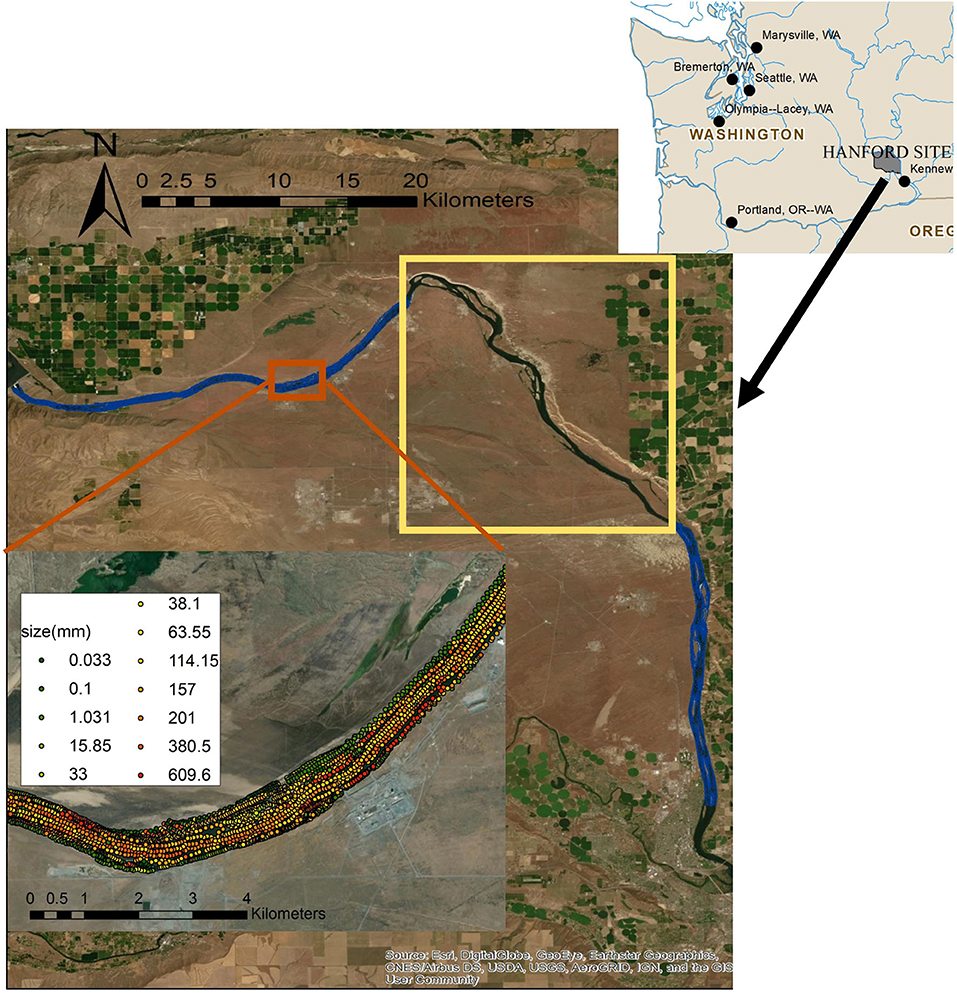
Figure 1. The location of substrate size samples along the Hanford Reach of the Columbia River. The blue dots are the sampling locations and the yellow box is the region without samples. The enlarged subplot shows the substrate size distribution.
Dominant Substrate Size
USFWS conducted survey operations along the reach to characterize grain size distributions in terms of dominant substrate sizes (Anglin et al., 2006; Hou et al., 2019) to study fish habitats. To determine the dominant substrate size, each one square meter area was evaluated by assigning a representative grainsize range equal to the median grain size D50. For water depths >0.5 m, the riverbed was photographed to capture the substrate grain size, and for water depths >0.5 m, the grain size was determined by wading the stream. Over 59 river kilometers, 13,372 locations were sampled and one-third of the sampling locations were in water deep enough to require underwater video sampling (Anglin et al., 2006). Twelve grain size classes were identified—from 0.033 to 609.6 mm—as listed in Table 1, and were further lumped to four groups by adopting the particle size classification according to the U.S. Geological Survey's recommendation (Berenbrock and Tranmer, 2008); i.e., silt (0.033 mm), sand (0.062–2.0 mm), gravel (2.0–64 mm), and cobble (>64 mm). The silt group contains only class 1 (i.e., coarse silt); the sand category contains classes 2 and 3; gravel contains classes 4–7; and cobble contains the rest of the classes 8–12. The spatial resolution of the samples varies from 50 to 70 m and the sampling locations cover ~70% of the entire Hanford Reach, as shown in the blue regions in Figure 1. The regions without samples are marked in the yellow boxed section.
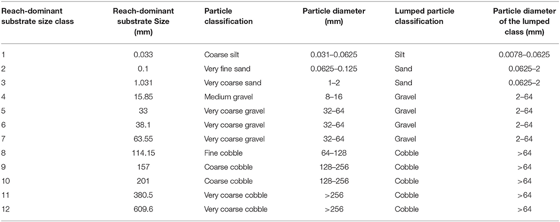
Table 1. Substrate size classification.
Bathymetric Attributes
Riverbed digital elevation data have been obtained from prior combined LiDAR and bathymetric surveys on a grid resolution of 1 m (Coleman et al., 2010). The bathymetric derivatives were extracted from the digital elevation survey data. For each grid cell, the slope and aspect were calculated using the “Slope” and “Aspect” tool of the Environmental Systems Research Institute ArcGIS platform. Slope describes the steepness of a grid cell in a raster surface. It is calculated as the inverse tangent of the rise divided by the run, with the higher value representing steeper terrain. Aspect represents the compass direction of a slope and is measured clockwise from 0 to 360 degrees. It is the downslope direction of the maximum rate of change in value from each cell to its neighbors. Aspect variables of non-sloping flat surfaces are flagged with a value of −1. River bathymetry and bathymetric variability are likely to be related to riverbed dominant substrate size distributions, and therefore these bathymetric attributes were included as potential predictors in the ML model development.
Hydrodynamic Attributes
Hanford Reach hydrodynamics were simulated using the Modular Aquatic Simulation System 2D (MASS2) model (Perkins and Richmond, 2007a,b; Niehus et al., 2014). MASS2 is a two-dimensional, depth-averaged hydrodynamic model that uses an orthogonal curvilinear mesh. As part of the previous work, MASS2 was applied from Priest Rapids Dam to near the mouth of the Yakima River, ~97 km, using a computational mesh with ~710,000 cells and a nominal resolution of ~10 m. The bathymetry in the Hanford Reach was assumed to be very stable over the more than 100-year MASS2 simulation period based on the underlying geology (Fecht et al., 2004; Fecht and Marceau, 2006; Hou et al., 2019). MASS2 was calibrated using water surface elevations measured at selected locations along the Hanford Reach, with mean absolute errors ranging from 1 to 12 cm. The calibrated models were then used to simulate the Hanford Reach conditions for a long historical period for which discharge records are available. Model calibration and long-term simulation details are documented by Niehus et al. (2014). Hourly hydrodynamic results from 1917 to 2012 under various flow conditions in the Hanford Reach were available for each grid. The simulation outputs, including the wet percentage, water depth, velocity magnitude, bottom shear stress and shear velocity, and their statistical moments (i.e., mean, variance, skewness, and kurtosis), were used as the predictors of dominant substrate size distribution. Together with the bathymetric predictors and substrate size responses, all the hydrodynamic variables were mapped onto the MASS2 grids.
Random Forest Classification
Given the high dimensionality of the predictors and non-linear relationships between the substrate size and these predictors, we adopted a reliable ensemble tree-based approach called Random Forest (RF) in our problem. RF is an ensemble ML algorithm that uses a collection of decision trees as base classifiers (Breiman, 2001) {h(x, Θk), k = 1, 2, 3……}, where the Θk are independent identically distributed random vectors and x is the input vector that each tree casts a unit vote for the most popular class. To grow a RF, user-defined parameters are required, including the number of the trees (k) and the number of predictive variables used to split the nodes (m). Each tree is grown using the training data set, which is created using a bootstrap aggregating (bagging) technique to create the resampling randomly and uniformly from the original data with replacement, and is comprised of a series of decision nodes or branching points (Pal, 2005; Rodriguez-Galiano et al., 2012). Past studies have revealed that bagging methods, such as RF, are not sensitive to noises or outliers (Briem et al., 2002; Chan and Paelinckx, 2008). Because the random feature selection of RF offers correlation reduction between the features which makes RF not vulnerable to the inherent noise existing in the training data. Because there is no deletion of the data sampled from the inputs for creating the next subset, the bagging helps to achieve the stability of classifiers with high accuracy (Breiman, 2001; Gislason et al., 2006). The distribution of the input samples does not change because the bagging uses random resampling instead of reweighting. Each new training set is drawn, with replacement, from the original training set. Then a tree is grown on the new training set using random feature selection. The trees grown are not pruned. Thus, all training classifiers have equal weights during split (Breiman, 2001). The response y is predicted by taking the majority vote in the case of classification trees. When each subset is selected by bagging to grow each individual tree, the inputs that are not included in the training and calibration data set in the current growing tree are counted in an out-of-bag (OOB) data set. OOB is the mean prediction error on each training sample xi, using only the trees that did not have xi in their bootstrap sample. The proportion of misclassifications over all OOB data sets is called the OOB error, which is an unbiased estimation of the generalization error without separating the testing data (Breiman, 2001; Peters et al., 2007). To make the generalization error converge, the number of trees (k) needs to be large enough. For a large number of trees, convergence follows from the Strong Law of Large Numbers and the tree structure. The RF can address the overfitting issue by checking and assuring such error convergency. The strength of each individual tree and the correlation between any two trees are used to evaluate the generalization error by the best split of input features or predictive variables. The Gini index, a measure of the impurity of a given input feature with respect to the rest of the classes, is a popular quantity for the best split selection. One of the advantages of RF is that it allows individual decision trees to grow to the maximum depth using a given combination of features, because (Mingers, 1989; Pal, 2005). Meanwhile, the relative importance of features is provided during the classification process.
RF is well-suited for high-dimensional data sets and/or highly correlated input features and has been successfully applied to the soil microbial community, remote sensing classification, water resources, and so on (Heung et al., 2014; Naghibi et al., 2017; Tesoriero et al., 2017). Open-source statistical software R (R Core Team, 2013) was used in this study, where the R implementation of the RF package (Liaw and Wiener, 2002) was used for RF model development, validation, and prediction.
In our study, the variable vector y to be classified represents the riverbed substrate classes at various spatial locations along the Hanford Reach. The categorical variables of interest to be predicted y can be grouped into 12 classes or 4 lumped groups. The input vector x contains bathymetric and hydrodynamic attributes at the collocated positions with categorical variable vector y, ensemble decision trees are then constructed using the training dataset; The input variables are selected randomly to get the best split-point to split the node into child notes to grow each decision tree.
Results
ML Data Preparation and RF Model Development
There are 13,372 data samples of dominant substrate sizes collected in the study domain, grouped into 12 classes and 4 categories. These are the “labels” information for ML training. At these sampling locations, information about the predictors is extracted from the high-resolution data sets of bathymetry and hydrodynamics. The bathymetric attributes include local bathymetry, slope, and aspect. The hydrodynamic attributes from multi-year MASS2 simulation include the wet percentage, water depth, velocity magnitude, river bottom shear stress, and shear velocity, together with their first four statistical central moments (e.g., mean, variance, skewness, and kurtosis). All the bathymetric and hydrodynamic attributes are treated as input features for the ML RF model development and the output response variable is the categorical substrate grain size. The ML model builds the relationship between substrate size and the features using the available grain-size measurements. Although there are 13,372 data points, we consider it as a spatially “sparse” dataset as they are dispersed along a 70-km long reach and the adjacent points are usually dozens of meters away from each other. In order to fill the spatial gaps while mapping the substrate size, the developed ML model of grain size can be applied to the numerical grid, with 5–10 m spatial resolution, to enable grain size mapping with adequate spatial coverage and resolution. Note that the spatial coordinates information, e.g., the Easting and Northing cartesian coordinates, contains spatial adjacency information, and can potentially help improve the ML prediction accuracy; but this information should be excluded when considering the generality and transferability of the developed models.
The ML (RF) models were developed through comprehensive model optimization and cross-validation. Different model configurations have been evaluated and compared to achieve the highest performance metrics (e.g., accuracy) and minimum overfitting. For example, the effect of the number of trees (k) and the number of predictive variables of the split nodes (m) were evaluated by six RF models, each of them constructed from up to 10,000 trees for each different value of m. The original database was randomly separated with 85% of the data points used for training and the remaining 15% held back for the testing data set. Figure 2 shows the OOB error with respect to the number of trees using the training data set with different predictive variables and the minimum size of terminal nodes set to 10. Here the minimum size of the terminal node implicitly sets the depth of trees in the model. The OOB error decreases significantly as the number of trees grows to 200 for all cases. When the number of predictive variables m is three, the OOB error is higher than the rest of the cases regardless of the number of trees. The error variability becomes very small when there are more than 1,000 trees. In the finalized optimal RF model configurations, m is set to be 15 with the lowest OOB errors and the tree number is set to be 1,000.

Figure 2. The OOB error with respect to number of trees for different predivtive variables for split node (m).
RF Parameter Ranking and Model Performance
Figure 3 shows the ranked variable importance based on the RF classification. The left panel is the Mean Decrease in Accuracy (MDA), which measures the loss of accuracy by taking variables out one by one. A high value of MDA means that the variable improves the model accuracy. The mean bathymetry is clearly the most important variable, followed by the bathymetric attributes, slope and aspect, water depth's third moment. The right panel in Figure 3 is the mean decrease in Gini impurity (MDG), which provides both variable contributions to the accuracy and the degree of misclassification. Important predictors correspond to high MDGs. Gini impurity achieves zero if all the responses in the training data in a group fall into a single category (i.e., no classification). The top variable according to MDG is the mean bathymetry, followed by four comparative factors: the slope of bathymetry, the third moment of water depth, aspect and water depth. Based on both the MDA and MDG variable importance, we can conclude that the flow conditions (water depth and its third moment) and the bathymetric attributes are the most influential factors. In addition, the velocity and the kurtosis of bottom shear stress are relatively important. The wet percentage is secondary but not negligible in terms of MDG.
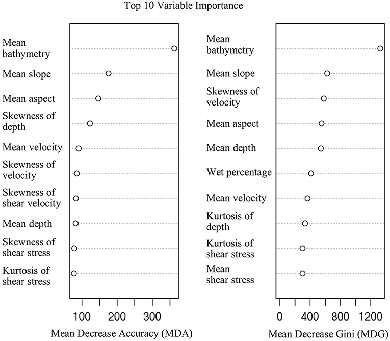
Figure 3. Dot chart of the top 10 features importance as measured by the RF model trained in optimized configuration.
The testing data set was used to evaluate the RF model accuracy in predicting the 12 classes and 4 categories of substrate sizes. The histogram of model predictions is illustrated for each individual class in Figure 4. The red bar represents the correct classifications/predictions for each class (classes 1–12) and the blue bars are the additional correct classifications/predictions of each category (silt, sand, gravel, and cobble). In general, the majority of RF predictions of the individual classes are correct; i.e., the red bar has the most counts and the correct classification cases dominate. The second highest bars generally also fall in the same lumped categories, e.g., the blue bars have the second largest values in each category except for classes 2 and 3. This means even if the RF model does not predict correctly the exact class (1–12), it most likely can still predict the correct silt/sand/gravel/cobble category.
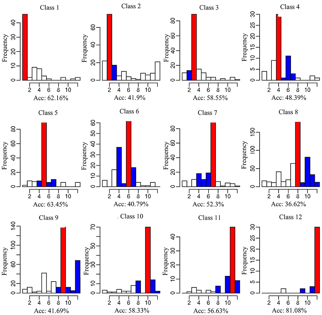
Figure 4. RF prediction for each substrate class. The red bar represents each targeted class. The blue bins represent the classes lumped by silt (class 1), sand (classes 2 and 3), gravel (classes 4 ~ 7), and cobble (classes 8 ~ 12). The accuracy of each individual class prediction is listed for each subplot.
Quantitatively, the classification accuracy for individual class ranges from 36 to 81% with a mean accuracy of 53%. Class 8 (substrate size class of 114.15 mm, fine cobble), containing the largest number of testing sample size, had the lowest accuracy. Although 170 testing samples were predicted correctly to fall under class 8, the RF model predicted about 70 samples fall under class 10 (coarse cobble). The model exhibits the best performance for class 12 with the largest substrate size class of 609.6 mm and is labeled as very coarse cobble. Meanwhile, for class 6 (very coarse gravel with a 63.44 mm substrate size class), ~40 samples were predicted to fall under class 4 (medium gravel). Similar observations were seen for class 7 as well. The medium gravel class 4 had 30 samples that were classified correctly while ~15 samples were misclassified into class 6. The model performance is summarized for the four lumped categories in Figure 5. The overall prediction accuracies for the silt, sand, gravel, and cobble categories are 62, 59, 79, and 71%, respectively. The model performance is satisfactory, although the uncertainty of substrate size distribution is large in the raw data and can be attributed non-linearly to many factors that have strong cross-dependence.
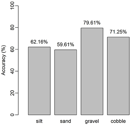
Figure 5. RF prediction accuracy for the four lumped groups: silt, sand, gravel, and cobble.
Spatial Mapping of Substrate Grain Size
Based on the field observations and simulations, we have developed an RF model representing the non-linear relationships between the substrate size and bathymetric and hydrodynamic attributes. The validated and tested RF model can be adopted and applied to all the numerical grids of 5–10 m resolution across the entire Hanford Reach. As a verification, Figure 6 shows a subsection of four river kilometers that have multiple hydromorphic features (e.g., island, attached bar, and meander), illustrating the comparison between the ground-truthing at a coarse spatial resolution and the model prediction on the finer grids. In Figure 6, the distributions of dominant substrate size are shown in 12 color-coded classes, where a larger substrate size corresponds to a larger class number. From the field observations shown in the left panel of Figure 6, class 1 (silt) grids are mainly located near the left banks of the shorelines between the meander and the island and near the right banks after the attached bar, corresponding to more of a depositional environment. For comparison, the model predictions on the grids in the right-hand panel of Figure 6 exhibit very similar patterns. Near a river segment below the island, where no USFWS measurements were available, the RF model predicts the substrate size to have a high probability of being silt. This is realistic by checking the patterns of the actual sampled locations relative to the bars and islands and our boat-based field survey. The sampling locations of class 2 grain sizes (fine sand) are along both sides of the river shoreline, especially on the right bank near the meander and on the left bank of the river below the gravel bar. Class 3 (coarse sand) tends to follow the same distribution of class 2, although it is farther away from the right riverbank near the meander. A few samples of class 4 were located near the tail of the island and no samples of class 5 were taken in this section of the river. Classes 6 and 7 have very few samples, and they are mainly located next to the island. The places with smaller substrate sizes concentrate more on the left shoreline than on the right shoreline. The most frequent samples in this subsection are class 8 (fine cobble), scattered in the river channel, around the island, near the front of the attached bar, and along both sides of the river channel. The sampling locations for coarse cobble including classes 9 and 10 are mainly located near the head of the island and the middle of the river channel. Most of the very coarse cobble locations are along the left shoreline near the meander and along the right-side bars behind the island. Compared to the ground-truthing data, the RF model predictions produce realistic spatial patterns and reflect reasonable spatial heterogeneity. Additional validation of RF predictions of substrate size categories (silt, sand, gravel, cobble) is shown in Figure 7. Generally, the gravel group has a smaller proportion in the predictions than in the field observations in this region. The gravel sampled at the front of the island and left side of the meander area are all classified correctly. In the river channel, mostly cobble is predicted, which is consistent with the field observations. Meanwhile, the spatial variability and heterogeneity can be seen. Such information about heterogeneity in the permeability field enables the development of more realistic and accurate numerical models, rather than assuming uniform or block-wise uniform permeability values.
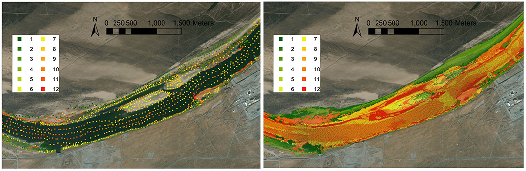
Figure 6. The dominant substrate size distribution of 12 classes with smaller class number representing the smaller dominant substrate size. The left panel is the ground-truthing and the right panel is the model prediction for each simulation grid.
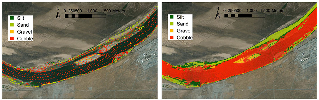
Figure 7. The dominant substrate size distribution of the four lumped classes. The left panel is the ground-truthing and the right panel is the model prediction for each simulation grid.
Discussion
In order to avoid over-fitting in the developed ML models, the ensemble bagging-based RF model was adopted to build the relationships between dominant substrate size and influential factors including bathymetric and hydrodynamic elements. Although RF models have been proven to be effective in terms of prediction accuracy and handling of overfitting issues, it is helpful to compare its performance with other ML approaches, particularly other widely accepted ensemble ML models, such as the boosting-based Extreme Gradient Boosting Model (GBM) (Chen et al., 2015). GBM is also tree-based, but the difference between RF and GBM is that the latter builds one tree at a time, and each tree learns and improves upon the previous one and combines results throughout the tree-building process. The disadvantage of GBM is that it is computationally expensive and sensitive to noises in the data set. Parameter tuning is performed for GBM with respect to the number of trees, the maximum tree depth, and the subsample ratio of columns when constructing each tree. The model accuracy obtained from the cross validation is shown in Figure 8. Each subplot in Figure 8 represents the different subsample ratio of columns when each tree was constructed. The x axis of each subplot is maximum tree depth which controls the depth of each individual tree. The different number of trees are color coded under each subplot showing different boosting iterations. The highest GBM model accuracy is about 55.6% with the optimized parameters, where the maximum tree depth is 10, the total number of trees is about 200, and the subsample ratio of columns is 0.9. The model accuracy for the four lumped substrate size categories using GBM and RF is compared in Table 2, which shows that the GBM and RF model prediction accuracies are generally comparable. RF is better at predicting finer materials such as silt, while GBM has stronger skill for predicting coarse cobble. For both methods, the lowest accuracy occurs when the dominant substrate size is <0.0625 mm (i.e., silt), while the highest accuracy (>80%) occurs when the substrate size is in the cobble group, which means the larger dominant substrate size group is relatively easier to predict using the available predictors, likely because the corresponding grains are well-sorted and subject to small variability.
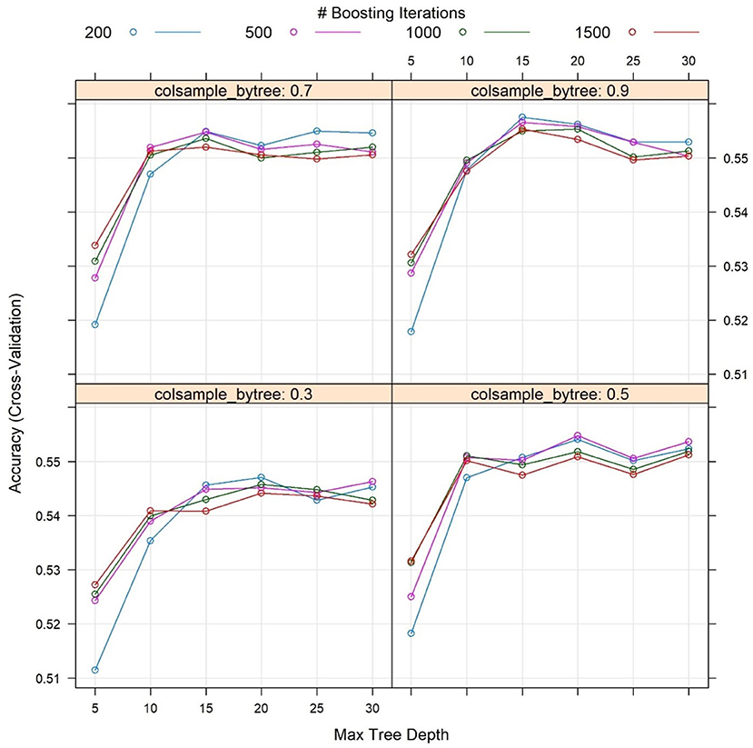
Figure 8. The cross-validation accuracy of the Extreme Gradient Boosting Model (GBM) achieved by tuning the maximum tree depth (x axis), number of trees (different colored lines), and subsample ratio of columns (noted as subtitle “colsample_by tree” for each subplot) when constructing each tree.
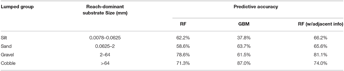
Table 2. Predictive accuracy of lumped four groups with different model setups.
Table 2 shows satisfactory testing accuracy for the testing grids/domain and proven transferability of the developed models. Although in the prediction model we did not include the spatial coordinate information, we did investigate the impact of adding spatial coordinates such as the Northing and Easting coordinate information in the predictor list and repeated the model training and testing. With the RF model, about a 3% improvement in the prediction accuracy was achieved by adding the spatial adjacency information for the finer silt, gravel, and cobble categories. The adjacency information provides more help for the sand category with a 7% increase in the prediction accuracy.
Therefore, spatial substrate grain-size distributions can be reasonably predicted using ML models on high-resolution numerical simulation grids. The spatial map of grain size can then be used to estimate hydraulic properties at the same resolution. The limitations of the approach, on the other hand, include the fact that the field observations of substrate size used in the model development mainly deliver valuable information of 2D spatial patterns near the top of the riverbed (Brunner et al., 2017). Without integration of vertical structural information, the approach seems to have overestimated hydraulic conductivity using grain-size distribution; meanwhile, the approach did not fully consider the degree of anisotropy and preferential flow pathways (Gianni et al., 2019). Given the transient nature of the system, the reliability of the estimation for hydraulic properties may also be affected by the system flow scenarios (Gianni et al., 2016). Nevertheless, our estimates of hydraulic properties can provide reliable inputs with reduced uncertainty toward improved numerical models in both accuracy and precision. This top of the permeability field is one of the most influential factors that control the magnitude (Lackey et al., 2015; Bao et al., 2018), spatial extent (Schilling et al., 2017), and associated biogeochemical hot spots (Song et al., 2018; Dai et al., 2019) of HEFs.
Conclusion
In this work, we developed an ML approach to predict dominant substrate size distribution, which enables to map the permeability field in the Hanford Reach of the Columbia River, providing more accurate and reliable inputs of the heterogeneous property field to the numerical models to obtain more realistic HEFs in river corridor systems. The developed ML models can link dominant substrate size to the available bathymetric and hydrodynamic attributes with high resolution. The traditional geostatistical approach is not applicable to the study site because of the large spatial gaps in the un-sampled locations. Therefore, our ML-based algorithms fill the gaps in mapping spatial grain-size distribution using the abundant indirect information available to us.
Given the satisfactory prediction accuracy of the testing data set, the generated substrate size can reliably provide the needed heterogeneous property input information based on well-reported and calibrated relationships between hydraulic properties and substrate grain-size distributions, which allows the numerical models to evaluate the effects of spatial heterogeneity on model outputs (e.g., HEFs, residence times), and enables a better understanding of the complex hydrological river corridor system.
Data Availability Statement
The datasets presented in this study can be found in online repositories. The names of the repository/repositories and accession number(s) can be found below: SBR SFA PNNL data repository https://sbrsfa.velo.pnnl.gov/datasets/?UUID=a165e7a4-427d-4997-845f-032d61975d85.
Author's Note
Pacific Northwest National Laboratory is operated by Battelle Memorial Institute for the U.S. Department of Energy under Contract No. DE-AC05-76RL01830. Hydrodynamic modeling of the Hanford Reach was performed for Public Utility District No. 2 of Grant County, Ephrata, WA, USA, under contract number 430-2464.
Author Contributions
HR and ZH contributed to the design and implementation. ZD processed the bathymetric attributes and generated some plots. WP and MR simulated hydrodynamics. XS and TS discussed the results and commented on the manuscript. All authors contributed to writing the manuscript.
Funding
This research was supported by the U.S. Department of Energy, Office of Biological and Environmental Research (BER), as part of BER's Subsurface Biogeochemical Research Program (SBR). This contribution originates from the SBR Scientific Focus Area at the Pacific Northwest National Laboratory (PNNL).
Conflict of Interest
The authors declare that the research was conducted in the absence of any commercial or financial relationships that could be construed as a potential conflict of interest.
References
Anglin, D. R., Haeseker, S. L., Skalicky, J. J., Schaller, H., Tiffan, K. F., Hatten, J. R., et al. (2006). Effects of Hydropower Operations on Spawning Habitat, Rearing Habitat, and Standing/Entrapment Mortality of Fall Chinook Salmon in the Hanford Reach of the Columbia River. US Fish and Wildlife Service.
Arntzen, E. V., Geist, D. R., and Dresel, P. E. (2006). Effects of fluctuating river flow on groundwater/surface water mixing in the hyporheic zone of a regulated, large cobble bed river. River Res. Appl. 22, 937–946. doi: 10.1002/rra.947
Bao, J., Zhou, T., Huang, M., Hou, Z., Perkins, W., Harding, S., et al. (2018). Modulating factors of hydrologic exchanges in a large-scale river reach: Insights from three-dimensional computational fluid dynamics simulations. Hydrol. Process. 32, 3446–3463. doi: 10.1002/hyp.13266
Berenbrock, C., and Tranmer, A. W. (2008). Simulation of Flow, Sediment Transport, and Sediment Mobility of The Lower Coeur d'Alene River, Idaho. Reston, VA: US Geological Survey.
Boano, F., Harvey, J. W., Marion, A., Packman, A. I., Revelli, R., Ridolfi, L., et al. (2014). Hyporheic flow and transport processes: mechanisms, models, and biogeochemical implications. Rev. Geophys. 52, 603–679. doi: 10.1002/2012RG000417
Boulton, A. J., Findlay, S., Marmonier, P., Stanley, E. H., and Valett, H. M. (1998). The functional significance of the hyporheic zone in streams and rivers. Annu. Rev. Ecol. Syst. 29, 59–81. doi: 10.1146/annurev.ecolsys.29.1.59
Briem, G. J., Benediktsson, J. A., and Sveinsson, J. R. (2002). Multiple classifiers applied to multisource remote sensing data. IEEE Trans. Geosci. Remote Sens. 40, 2291–2299. doi: 10.1109/TGRS.2002.802476
Brunke, M., and Gonser, T. (1997). The ecological significance of exchange processes between rivers and groundwater. Freshw. Biol. 37, 1–33. doi: 10.1046/j.1365-2427.1997.00143.x
Brunner, P., Therrien, R., Renard, P., Simmons, C. T., and Franssen, H. J. H. (2017). Advances in understanding river-groundwater interactions. Rev. Geophys. 55, 818–854. doi: 10.1002/2017RG000556
Cardenas, M. B., Wilson, J., and Zlotnik, V. A. (2004). Impact of heterogeneity, bed forms, and stream curvature on subchannel hyporheic exchange. Water Resour. Res. 40:W08307. doi: 10.1029/2004WR003008
Chan, J. C.-W., and Paelinckx, D. (2008). Evaluation of Random Forest and Adaboost tree-based ensemble classification and spectral band selection for ecotope mapping using airborne hyperspectral imagery. Remote Sens. Environ. 112, 2999–3011. doi: 10.1016/j.rse.2008.02.011
Chen, T., He, T., Benesty, M., Khotilovich, V., and Tang, Y. (2015). Xgboost: Extreme Gradient Boosting. R package version 0.4-2, 1–4.
Chen, X. (2000). Measurement of streambed hydraulic conductivity and its anisotropy. Environ. Geol. 39, 1317–1324. doi: 10.1007/s002540000172
Cheng, C., Song, J., Chen, X., and Wang, D. (2011). Statistical distribution of streambed vertical hydraulic conductivity along the Platte River, Nebraska. Water Res. Manag. 25, 265–285. doi: 10.1007/s11269-010-9698-5
Coleman, A. M., Ward, D. L., Larson, K. B., and Lettrick, J. W. (2010). “Development of a high-resolution bathymetry dataset for the Columbia River through the Hanford Reach,” in Pacific Northwest National Lab, (Richland, WA: Pacific Northwest National Laboratory).
Dai, H., Chen, X., Ye, M., Song, X., Hammond, G., Hu, B., et al. (2019). Using Bayesian networks for sensitivity analysis of complex biogeochemical models. Water Resour. Res. 55, 3541–3555. doi: 10.1029/2018WR023589
Fecht, K., Marceau, T., Bjornstad, B., Horton, D., Last, G., Peterson, R., et al. (2004). Late Pleistocene and Holocene-Age Columbia River Sediments and Bedforms: Hanford Reach Area, Washington, Part 1: Richland. Washington, DC: Bechtel Hanford. Inc.
Fecht, K., and Marceau, T. (2006). Late Pleistocene and Holocene-Age Columbia River Sediments and Bedforms: Hanford Reach Area, Washington-Part 2. Washington Closure Hanford.
Fritz, B. G., and Arntzen, E. V. (2007). Effect of rapidly changing river stage on uranium flux through the hyporheic zone. Groundwater 45, 753–760. doi: 10.1111/j.1745-6584.2007.00365.x
Fritz, B. G., Mackley, R. D., and Arntzen, E. V. (2016). Conducting slug tests in mini-piezometers. Groundwater 54, 291–295. doi: 10.1111/gwat.12335
Gianni, G., Doherty, J., and Brunner, P. (2019). Conceptualization and calibration of anisotropic alluvial systems: pitfalls and biases. Groundwater 57, 409–419. doi: 10.1111/gwat.12802
Gianni, G., Richon, J., Perrochet, P., Vogel, A., and Brunner, P. (2016). Rapid identification of transience in streambed conductance by inversion of floodwave responses. Water Resour. Res. 52, 2647–2658. doi: 10.1002/2015WR017154
Gislason, P. O., Benediktsson, J. A., and Sveinsson, J. R. (2006). Random forests for land cover classification. Pattern Recognit. Lett. 27, 294–300. doi: 10.1016/j.patrec.2005.08.011
Harvey, J., and Gooseff, M. (2015). River corridor science: hydrologic exchange and ecological consequences from bedforms to basins. Water Resour. Res. 51, 6893–6922. doi: 10.1002/2015WR017617
Hayashi, M., and Rosenberry, D. O. (2002). Effects of ground water exchange on the hydrology and ecology of surface water. Groundwater 40, 309–316. doi: 10.1111/j.1745-6584.2002.tb02659.x
Heung, B., Bulmer, C. E., and Schmidt, M. G. (2014). Predictive soil parent material mapping at a regional-scale: a random forest approach. Geoderma 214, 141–154. doi: 10.1016/j.geoderma.2013.09.016
Hou, Z., Nelson, W. C., Stegen, J. C., Murray, C. J., Arntzen, E., Crump, A. R., et al. (2017). Geochemical and microbial community attributes in relation to hyporheic zone geological facies. Sci. Rep. 7:12006. doi: 10.1038/s41598-017-12275-w
Hou, Z., Scheibe, T. D., Murray, C. J., Perkins, W. A., Arntzen, E. V., Ren, H., et al. (2019). Identification and mapping of riverbed sediment facies in the Columbia River through integration of field observations and numerical simulations. Hydrol. Process. 33, 1245–1259. doi: 10.1002/hyp.13396
Irvine, D. J., Brunner, P., Franssen, H.-J. H., and Simmons, C. T. (2012). Heterogeneous or homogeneous? Implications of simplifying heterogeneous streambeds in models of losing streams. J. Hydrol. 424, 16–23. doi: 10.1016/j.jhydrol.2011.11.051
Kasahara, T., and Wondzell, S. M. (2003). Geomorphic controls on hyporheic exchange flow in mountain streams. Water Res. Res. 39, SBH 3-1–SBH 3-14. doi: 10.1029/2002WR001386
Kasenow, M. (2002). Determination of Hydraulic Conductivity From Grain Size Analysis. Water Resources Publication.
Lackey, G., Neupauer, R. M., and Pitlick, J. (2015). Effects of streambed conductance on stream depletion. Water 7, 271–287. doi: 10.3390/w7010271
Landon, M. K., Rus, D. L., and Harvey, F. E. (2001). Comparison of instream methods for measuring hydraulic conductivity in sandy streambeds. Groundwater 39, 870–885. doi: 10.1111/j.1745-6584.2001.tb02475.x
Lu, C., Chen, X., Cheng, C., Ou, G., and Shu, L. (2012). Horizontal hydraulic conductivity of shallow streambed sediments and comparison with the grain-size analysis results. Hydrol. Process. 26, 454–466. doi: 10.1002/hyp.8143
Malcolm, I., Soulsby, C., Youngson, A., and Petry, J. (2003). Heterogeneity in ground water–surface water interactions in the hyporheic zone of a salmonid spawning stream. Hydrol. Process. 17, 601–617. doi: 10.1002/hyp.1156
McCallum, A. M., Andersen, M. S., Rau, G. C., Larsen, J. R., and Acworth, R. I. (2014). River-aquifer interactions in a semiarid environment investigated using point and reach measurements. Water Resour. Res. 50, 2815–2829. doi: 10.1002/2012WR012922
Mingers, J. (1989). An empirical comparison of selection measures for decision-tree induction. Mach. Learn. 3, 319–342. doi: 10.1007/BF00116837
Naghibi, S. A., Ahmadi, K., and Daneshi, A. (2017). Application of support vector machine, random forest, and genetic algorithm optimized random forest models in groundwater potential mapping. Water Res. Manag. 31, 2761–2775. doi: 10.1007/s11269-017-1660-3
Niehus, S., Perkins, W., and Richmond, M. (2014). Simulation of Columbia River Hydrodynamics and Water Temperature From 1917 Through 2011 in the Hanford Reach. Final Report PNWD-3278, Battelle-Pacific Northwest Division. Richland, WA.
Odong, J. (2007). Evaluation of empirical formulae for determination of hydraulic conductivity based on grain-size analysis. J. Am. Sci. 3, 54–60.
Pal, M. (2005). Random forest classifier for remote sensing classification. Int. J. Remote Sens. 26, 217–222. doi: 10.1080/01431160412331269698
Perkins, W. A., and Richmond, M. C. (2007a). MASS2, Modular Aquatic Simulation System in Two Dimensions, Theory and Numerical Methods. Richland, WA: Pacific Northwest National Lab(PNNL).
Perkins, W. A., and Richmond, M. C. (2007b). MASS2, Modular Aquatic Simulation System in Two Dimensions, User Guide and Reference. Richland, WA: Pacific Northwest National Lab(PNNL).
Peters, J., De Baets, B., Verhoest, N. E., Samson, R., Degroeve, S., De Becker, P., et al. (2007). Random forests as a tool for ecohydrological distribution modelling. Ecol. Modell. 207, 304–318. doi: 10.1016/j.ecolmodel.2007.05.011
Rodriguez-Galiano, V. F., Ghimire, B., Rogan, J., Chica-Olmo, M., and Rigol-Sanchez, J. P. (2012). An assessment of the effectiveness of a random forest classifier for land-cover classification. ISPRS J. Photogramm. Remote Sens. 67, 93–104. doi: 10.1016/j.isprsjprs.2011.11.002
Salehin, M., Packman, A. I., and Paradis, M. (2004). Hyporheic exchange with heterogeneous streambeds: Laboratory experiments and modeling. Water Resour. Res. 40:W11504. doi: 10.1029/2003WR002567
Sawyer, A. H., and Cardenas, M. B. (2009). Hyporheic flow and residence time distributions in heterogeneous cross-bedded sediment. Water Resour. Res. 45:W08406. doi: 10.1029/2008WR007632
Schilling, O. S., Irvine, D. J., Hendricks Franssen, H. J., and Brunner, P. (2017). Estimating the spatial extent of unsaturated zones in heterogeneous river-aquifer systems. Water Resour. Res. 53, 10583–10602. doi: 10.1002/2017WR020409
Shepherd, R. G. (1989). Correlations of permeability and grain size. Groundwater 27, 633–638. doi: 10.1111/j.1745-6584.1989.tb00476.x
Song, X., Chen, X., Stegen, J., Hammond, G., Song, H. S., Dai, H., et al. (2018). Drought conditions maximize the impact of high-frequency flow variations on thermal regimes and biogeochemical function in the hyporheic zone. Water Resour. Res. 54, 7361–7382. doi: 10.1029/2018WR022586
Sophocleous, M. (2002). Interactions between groundwater and surface water: the state of the science. Hydrogeol. J. 10, 52–67. doi: 10.1007/s10040-001-0170-8
Tang, Q., Kurtz, W., Brunner, P., Vereecken, H., and Franssen, H.-J. H. (2015). Characterisation of river–aquifer exchange fluxes: the role of spatial patterns of riverbed hydraulic conductivities. J. Hydrol. 531, 111–123. doi: 10.1016/j.jhydrol.2015.08.019
Tang, Q., Kurtz, W., Schilling, O., Brunner, P., Vereecken, H., and Franssen, H.-J. H. (2017). The influence of riverbed heterogeneity patterns on river-aquifer exchange fluxes under different connection regimes. J. Hydrol. 554, 383–396. doi: 10.1016/j.jhydrol.2017.09.031
Tang, Q., Schilling, O. S., Kurtz, W., Brunner, P., Vereecken, H., and Hendricks Franssen, H. J. (2018). Simulating flood-induced riverbed transience using unmanned aerial vehicles, physically based hydrological modeling, and the ensemble kalman filter. Water Resour. Res. 54, 9342–9363. doi: 10.1029/2018WR023067
Keywords: machine learning, random forest, spatial heterogeneity, grain-size distribution, riverbed permeability, hydrologic exchange flows (HEFs)
Citation: Ren H, Hou Z, Duan Z, Song X, Perkins WA, Richmond MC, Arntzen EV and Scheibe TD (2020) Spatial Mapping of Riverbed Grain-Size Distribution Using Machine Learning. Front. Water 2:551627. doi: 10.3389/frwa.2020.551627
Received: 14 April 2020; Accepted: 07 October 2020;
Published: 23 November 2020.
Edited by:
Alexis Navarre-Sitchler, Colorado School of Mines, United StatesReviewed by:
Alberto Bellin, University of Trento, ItalyOliver Schilling, Université de Neuchâtel, Switzerland
Copyright © 2020 Ren, Hou, Duan, Song, Perkins, Richmond, Arntzen and Scheibe. This is an open-access article distributed under the terms of the Creative Commons Attribution License (CC BY). The use, distribution or reproduction in other forums is permitted, provided the original author(s) and the copyright owner(s) are credited and that the original publication in this journal is cited, in accordance with accepted academic practice. No use, distribution or reproduction is permitted which does not comply with these terms.
*Correspondence: Huiying Ren, aHVpeWluZy5yZW5AcG5ubC5nb3Y=