 María González-Sanchis1,2*
 Juan M. García-Soro1,2
 Antonio J. Molina1,2
 Antonio L. Lidón1Inmaculada Bautista1Elie Rouzic3
 Heye R. Bogena4
 Harrie-JanHarrie Hendricks Franssen4Antonio D. del Campo1,2
- 1Research Group in Forest Science and Technology (Re-ForeST), Research Institute of Water and Environmental Engineering (IIAMA), Universitat Politècnica de València, Valencia, Spain
- 2Environmental Hydraulics Department, Universitat Politècnica de València (UPV), Valencia, Spain
- 3École Nationale Supérieure de Techniques Avancées (ENSTA Paris), Paris, France
- 4Agrosphere Institute (Institute of Bio- and Geosciences), Forschungszentrum Jülich, Jülich, Germany
Water scarcity in semi-arid regions is expected to increase under climate change, which will significantly affect forest ecosystems by increasing fire risk, diminishing productivity and water provisioning. Eco-hydrological forest management is conceived here as an adequate strategy to buffer climate change effects and increase forest resilience. Under this context, soil moisture is a key variable to quantify the impacts of eco-hydrological forest management on forest-water relations. Cosmic-ray neutron and capacitance probes are two different techniques for measuring soil moisture, which differ greatly in the spatial scale of the measurement support (i.e., few centimeters vs. several hectares). This study compares the capability of both methodologies in assessing soil water dynamics as a key variable that reflects the effects of forest management in a semi-arid environment. To this end, two experimental plots were established in Sierra Calderona in the province of Valencia in Spain in a post-fire regeneration Aleppo pine forest with high tree density. One plot was thinned (T) and the other remained as control (C). Nine capacitance probes and one Cosmic Ray Neutron Probe (CRNP) were installed in each plot. First, the CRNP was calibrated and validated, and subsequently, the performance of both techniques was analyzed by comparing soil moisture and its relationship with environmental variables and stand transpiration. The validation results confirmed the general reliability of CRNP to obtain soil moisture under semi-arid conditions, with a Kling-Gupta efficiency coefficient (KGE) between 0.75 and 0.84, although this performance decreased significantly when dealing with extreme soil moisture (KGE: −0.06–0.02). A significant effect of forest biomass and litter layer was also observed on CRNP-derived soil moisture, which produced an overestimation of soil moisture. The performance of both methodologies was analyzed by partial correlations between soil moisture and environmental variables and transpiration, as well as by applying Boosted Regression Trees to reproduce tree transpiration with each soil moisture measurement technique together with the environmental variables. Both methodologies were capable to reproduce tree transpiration affected by soil moisture, environmental variables and thinning, although CRNP always appeared as the most affected by atmospheric driving forces.
Introduction
Semi-arid forests are water-controlled environments where water availability has direct and indirect effects on key processes such as weathering, decomposition, soil respiration, nitrogen mineralization, nutrient uptake, biomass production, and long–term carbon sequestration (Rodríguez-Iturbe and Porporato, 2007). This water dependence leads these forests to face abiotic and biotic threats (e.g., wildfires, insect outbreaks and severe drought events) that may decline their capability to persist in their current geographic ranges, and to colonize new habitats (Bell et al., 2014; Rehfeldt et al., 2014). During the 20th Century, their persistence has been dependent on favorable climatic and environmental conditions (Savage et al., 1996; Mast et al., 1999; Brown and Wu, 2005), which unfortunately, according to climate change projections, are going to be less frequent, increasing the ecosystem threats and therefore diminishing its regeneration capability (Coops et al., 2005; van Mantgem et al., 2009; Williams et al., 2013). Under this context, adaptive forest management is conceived as useful strategy that shapes forest-water relationships to improve the capability of these forests to face the effects of climate change (del Campo et al., 2017).
Soil moisture can be an accurate proxy of water availability in a semi-arid forest as it is an important water source for vegetation development, and one of the most important factors controlling hydrological processes (Castillo et al., 2003; Seeger et al., 2004). Changes of soil water may greatly affect tree species diversity and forest canopy structure. In turn, changes in vegetation, which are often pursued in forest management, typically lead to changes in soil moisture. Therefore, soil moisture is a key variable in quantifying the impact of forest management on the forest-water relationship (del Campo et al., 2019b). There are different measuring methods to obtain reliable estimates of soil moisture, depending on the required spatio-temporal accuracy, ranging from direct manual measurements to satellite-based sensors (Vereecken et al., 2008). Time domain reflectometry (TDR) and capacitance sensors have been extensively used at the local scale (Gardner et al., 1998; Seyfried and Murdock, 2001; Topp and Ferré, 2006). Both are invasive methods that require several measurement points to estimate representative spatial and temporal mean soil water contents (Molina et al., 2014). In natural ecosystems, the need for a large number of measurement points is typically greater because the heterogeneity of soil moisture is larger compared to arable land, due to the typically greater differences in topography and vegetation cover, the uneven input of litter and the less intensive mixing of the soil (Hawley et al., 1983; Flinn and Marks, 2007). Alternatively, soil moisture sensors with larger measurement support could be used that are able to better cover the local scale variability, e.g., non-invasive methods like remote sensing or geophysical methods (Lv et al., 2014; Bogena et al., 2015). Although their capabilities are improving constantly, satellite based remote sensing currently shows lower accuracy than geophysical methods at the field to catchment scale (Lv et al., 2014). Therefore, when measuring soil moisture in forests, CRNP could be a compromise solution between spatial heterogeneity, accuracy and functionality.
The CRNP is a novel, non-invasive technique to measure the areal-averaged soil moisture of an effective depth in the order of decimeters within a radial footprint on the order of several hectares (Zreda et al., 2008; Andreasen et al., 2017). The CRNP are detectors that measure the fast neutron intensity at ground level generated by cosmic radiation (Heidbüchel et al., 2016). The interaction of fast neutrons with hydrogen atoms, which are mainly present in soil moisture, lowers the intensity of fast neutrons detected by the CRNP. Therefore an inverse relationship between neutron intensity and soil moisture exists that can be exploited to monitor soil moisture dynamics at the field scale (Bogena et al., 2013). According to Schrön et al. (2017), the CRNP provides indirect measurements of soil moisture over a circular footprint with an effective radius ranging approximately from 150 to 210 m (i.e., from about 7 to 14 hectares) depending on various factors, e.g., soil moisture, atmospheric pressure, air humidity, vegetation biomass etc. The contribution of neutron counts decreases rapidly with separation distance from the CRNP (Zreda et al., 2012), and ~50% of the cumulative fraction of neutron counts is contributed from distances <50 m (Schrön et al., 2017). The effective measurement depth strongly depends on soil water content (SWC), and decreases non-linearly from around 70–80 cm in dry soils to ~12 cm in saturated soils (Zreda et al., 2012). The CRNP is most sensitive to soil moisture in the upper soil horizon, and this sensitivity decreases exponentially with depth (Schrön et al., 2017).
Measurements of soil moisture with CRNP have been reported in many studies (e.g., Bogena et al., 2013; Hawdon et al., 2014; Lv et al., 2014; McJannet et al., 2014; Rosolem et al., 2014; Heidbüchel et al., 2016; Jana et al., 2016; Schreiner-McGraw et al., 2016; Wang et al., 2018), and around 60% have been carried out in crop or grasslands, 30% in forests and 11% in mixed forest-grassland ecosystems. Only 22% of these studies have been carried out under dry climates, such as semi-arid, and only 4% correspond to dry forests. Thus, there appears to be a gap of CRNP usage in semi-arid forests that alternate between very wet and very dry conditions. This inter-annual variation may strongly affect the effective penetration depth of CRNP, which is a particular challenge for the adequate interpretation of CRNP-derived soil moisture information (Schrön et al., 2017).
This study aims to contribute to filling this experimental gap by means of a dual objective dealing with the comparison between CRNP and capacitance sensors in a semi-arid forest, given their different spatial representativeness for (indirectly) measuring soil moisture content. On the one hand, we aim to analyze how the derived soil moisture from both methodologies is correlated with the environmental variables of the study area. On the other hand, we pursue to study which sensor is better indicating a physiological response to thinning and can therefore be used as a proxy of water availability in managed and unmanaged forests. To achieve this dual objective, the following secondary objectives were assessed: (a) to calibrate and validate CRNP through common procedures; (b) to study the degree of correlation between soil moisture (measured by CRNP or capacitance sensors) with different environmental variables like vegetation transpiration, and (c) to compare the potential explanatory power of CRNP and capacitance sensors when addressing the role of thinning on stand transpiration. To this end, the present work takes advantage of an experimental context that already exists in a pine stand growing under semi-arid conditions, where several measurements in the soil-plant-atmosphere continuum are taken in order to understand the role of thinning on tree-water relations (del Campo et al., 2019b; González-Sanchis et al., 2019).
Materials and Methods
Study Site and Forest Treatments
The study was carried out in a semi-arid forest with high tree density, located within the natural park of “La Sierra Calderona” (39°42“N, 0°27”W, altitude: 790 m asl) in the province of Valencia (Spain) (Figure 1). The existing vegetation is a young Aleppo pine stand with scattered shrubs (such as Quercus coccifera, Juniperus oxycedrus, and Ulex parviflorus) regenerated after a wildfire occurred in 1992. The climate is Mediterranean, characterized by high temporal rainfall variability and intense droughts (means of annual precipitation and potential evapotranspiration of 342 and 837 mm, respectively); with extreme dry years with cumulated precipitation lower than 150 mm. More information about vegetation, climate, soils and other bio-geographical traits is found in del Campo et al. (2018, 2019b) and González-Sanchis et al. (2019).
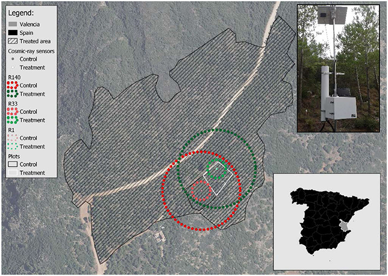
Figure 1. The experimental site within the “Sierra Calderona” Natural Park (Valencia, Spain). The dashed area indicates the treated area in 2012. R1, R33, and R140 indicate soil samplings with radii of 1, 33, and 140 m, respectively. The control and treatment plots are indicated by black and white line, respectively. The picture in the upper right shows one of the CRNP probes.
No forest management has been carried out since the 1992 wildfire, except for 2012 (between January and October) when a small portion of the forest was managed in the context of an experimental study and a contractor of the Forest Service executed juvenile thinning with shrub clearing. The thinning removed the trees with the smallest diameters and the double-stemmed trees (reduction of 74% of basal area or 94% of tree density) (Table 1), trying to achieve a relatively homogeneous forest cover distribution. The experimental design consisted of a representative control plot (C) with no thinning and a contiguous thinned plot (T), each of them having an area of 1,500 m2. Both plots have similar slope (27.8 vs. 32.0%) and aspect (311° vs. 319° NW). More details about forest structure can be found in del Campo et al. (2018, 2019b) and González-Sanchis et al. (2019).
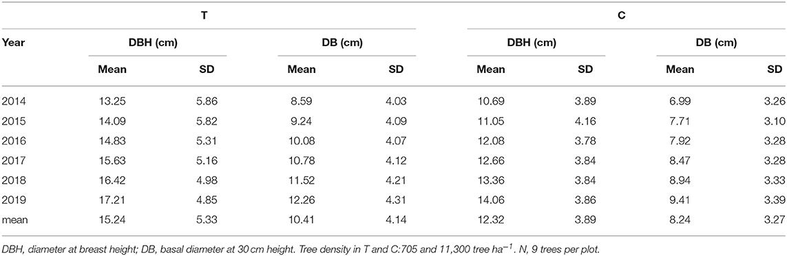
Table 1. Forest structure metrics (means and standard deviations) in control (C) and treatment (T) for the period between 2014 and 2019.
Measurements
Climatic Variables
Air temperature (T, °C) and relative humidity (RH, %) were measured (CS215, Campbell Sci., Decagon Devices, Pullman, WA, United States) in each experimental plot at two different heights, one at 2 m above the ground and the other at 6.5 m. Gross Precipitation (Pg, mm) was measured with a tipping-bucket (0.2 mm resolution) at 6 meters above the ground (7852, Davis Instruments Corp., Hayward, CA, United States). The net precipitation (Pn) has been calculated by the difference of Pg minus the canopy interception (It); the canopy interception was estimated to be 16.7 and 36.4% of Pg for T and C, respectively (del Campo et al., 2018). Wind speed (Ws, m s−1) and direction (Wd, °) were obtained using an anemometer (Anemometers 7911, Davis Instruments Corp.), located on the same mast measuring T and RH at 6.5 m above the ground. The sensors were connected to a data-logging unit (CR1000, Campbell Sci., UT, United States) supplemented with two AM16/32B Multiplexers, two SDM-IO16 expansion modules, a solar panel and a 12 V battery. Data was stored every 10 min. Vapor pressure deficit (VPD, kPa) was calculated following standard Equations (1–3) based on T and RH:
Where T is air temperature (°C), VPsat is the air saturated vapor pressure (kPa), VPair is the air vapor pressure (kPa) and VPD is the vapor pressure deficit (kPa).
Soil Moisture
Soil moisture (θ, m3 m−3) was continuously measured every 10 min, or every 5 s when raining, by means of capacitive probes (EC-5, Decagon Devices Inc., Pullman, WA) connected to a CR1000 data-logger. The EC-5 sensors were installed by digging nine pits per experimental plot (systematically placed), organized into three groups following contour lines (del Campo et al., 2019b). In each group, one of the pits contained two sensors poked horizontally at depths of 15 and 30 cm into the unaltered upslope pit face, whereas in the other two pits one sensor was poked at 15 cm depth (12 EC-5 sensors per plot, 24 EC-5 sensors per experimental site). The pits were regularly placed on a grid of 10 × 10 m to get a good estimate of mean soil moisture (Molina et al., 2014). After installation, the pits were backfilled with the excavated soils and slightly compacted to achieve a similar bulk density as the original, unaltered soil. As already reported in del Campo et al. (2018), a soil-specific calibration was not possible due to the stoniness at the field site, hence we used the standard EC-5 calibration (for mineral soils) in all cases (Detty and McGuire, 2010). For the validation of the CRNP, we considered the weighted θ average for each experimental plot based on the number of probes for each soil depth.
Stand Transpiration
Tree sap flow velocity (Vs, cm h−1) was measured every half hour by the heat ratio method (HRM) (Burgess et al., 2001). Eighteen home-made sap flow sensors were installed in 9 trees per plot [see González-Sanchis et al. (2019) for more details]. The sensors were installed on the upslope side at a height between 0.3 and 1 m. In addition, all sensors were connected to a data logger, a 12 V battery and a solar panel (CR1000, Campbell Sci., UT, United States). Sap flow (Sf) was obtained by calculating sapwood area (Sa, m−2) and up-scaling sap flow velocity (Vs, cm h−1) using the Excel macro provided by Berdanier et al. (2016). Subsequently, Sf was up-scaled to stand transpiration per plot (Tr, mm day−1) by using the number of trees (De, tree m−2) as scalar. We obtained a correction factor (cf) by regressing Sf on Sa (R2 > 91%) so that the Sf corresponding to the mean sampled tree was corrected to the mean plot tree (del Campo et al., 2019a).
Biomass Calculation at Plot Scale
Total biomass (Tb, kg m−2) was calculated using the allometric Equations (4–8) proposed by Ruiz-Peinado et al. (2011) for Pinus halepensis:
where Bs is the stem biomass, Bb7 is the biomass of thick branches (>7 cm of diameter), Bb7−2 is the biomass of medium branches (between 7 and 2 cm), Bb2+l is the biomass of small branches (<2 cm) and leaves, and Bb is the root biomass. d is de tree diameter at 1.30 m, h is tree height in meters and Z is 0 when d ≤ 27.5 cm, and 1 when d ≥ 27.5 cm.
Finally, Tb was calculated by summing up the different biomass parts of all trees and dividing this value by the area of each experimental plot.
Cosmic-Ray Neutron Sensors
Two CRNP (CRS-1000, Hydroinnova LLC, Albuquerque, NM, United States) were installed at the study site, one in the thinned (T) plot in January 2017, and the other one in the control (C) plot in June 2019 (Figure 1). In summary, the CRNP counts fast neutrons that enter the detector tube as indication for the local fast neutron intensity. The neutron count rate is corrected by the atmospheric pressure (Patm), the absolute water content in the air (Habs), the influence of the incoming neutrons (Inn) and finally, the influence of the amount of vegetation on these neutrons (fveg). For more details about CRNP see Bogena et al. (2013), Heidbüchel et al. (2016), and Zreda et al. (2008). This setup involved two different measurement periods for each experimental plot, January 1st 2017 to October 22th 2019 for the T plot, and June 17th 2019 to October 22th 2019 for the C plot. Therefore, CRNP data was simultaneously measured in both plots during a period of 4 months.
Sampling soil campaigns
The soil characterization at the experimental plots was carried out by collecting soil samples at four points in each plot, distributed along the slope and randomly selected in March 2013. At each point, a metal frame of 25 × 25 cm was used to collect separately the litter layer, the humified organic layer underneath and the top mineral soil layer from 0 to 5 cm. The deeper samples (from 5 to 20 cm and below 20 cm when possible) were taken with a 5 cm diameter helicoidal probe. Soil depth was highly variable from less of 20 cm to more than 70 cm. The samples were weighed, air dried and different fractions were separated by sieving through 2 mm mesh size. Air-dry soil humidity was determined in a subsample by drying at 105°C until constant weight. The larger fraction was separated (by hand) into stones, roots, leaf debris, woody debris and miscellaneous organic fraction. In the fine fraction, we determined soil pH in a 1:2.5 water suspension, inorganic carbonate content by the Bernard calcimeter method (MAPA, 1994), and total organic carbon (TOC) by the Walkey-Black method (Nelson and Sommers, 1982). The litter layer depth of C and T plots was measured at 9 points per plot, randomly distributed along the slope.
For CRNP calibration five soil samples were taken using different procedures. The first two sampling campaigns (T1 and T2) were carried out following the usual calibration procedure suggested by Bogena et al. (2013) which includes 18 extraction points distributed in 3 different circumferences (radius of 1, 33, and 140 m) whose center is CRNP, 6 extraction points per circumference (Figure 2). However, since the large volume of rock complicated the sampling procedure, during the rest of the sampling campaigns (T3, C1, and C2) the number of samples was reduced. This reduction was carried out attending to the significant differences between gravimetric humidity of samples from T1 and T2 campaigns. In these sense, sampling campaigns T3, C1, and C2 was carried out by sampling just in those extraction points were no significant differences between gravimetric humidity of T1 and T2 campaigns was observed (Figure 2B). As a result, sampling campaigns T3, C1, and C2 used 9 extraction points, while T1 and T2 collected samples at 18 points, both distributed within 3 sampling circumferences. At each sampling circumference, samples were collected in different orientations and depths. In T1 and T2, there were 18 extraction points in all directions (N, NE, NW, S, SE, and SW) and at all depths (0–5, 5–10, 10–15, 15–20, 20–25, 25–30), but for T3, C1, and C2, the direction was also reduced to N, SE, and SW (Figure 2).
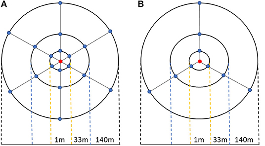
Figure 2. Schematic representation of the soil-sampling campaigns. The red point represent the CRNP probe while the blue ones are the sampling soil locations. (A) the calibration procedure described by Heidbüchel et al. (2016) (T1 and T2 samples); (B) new calibration procedure used in this study (T3, C1, and C2 samples).
Water equivalent of the belowground hydrogen content pools was obtained by considering composite samples for the six different soil depths from all sample locations (~2 g of soil from each location) (Heidbüchel et al., 2016). These soil samples were sieved through a 200 μm mesh size, oven-dried for 24 h at 105°C and weighted to determine the gravimetric water content. Subsequently, the soil samples were consecutively heated at 400, 700, and 1,000°C during 24 h to determine the contents of soil organic matter and lattice water. We included an intermediate step (700°C) to account for weight losses due to thermal break-down of carbonates at temperatures above 430°C because of the high carbonate content of the soil. Soil organic matter and root biomass content of each soil sample was obtained from the weight difference between the 105 and 400°C, and lattice water content by the weight difference between 700 and 1,000°C.
Cosmic-ray sensor neutrons correction and calibration
The first step was to correct the mean daily arrival of neutrons by the different equations proposed by Zreda et al. (2012) in order to account for the influence of atmospheric pressure (Equation 9), incoming neutrons (Equation 10) and air water vapor (Equation 11):
Where Np is the number of neutrons corrected for atmospheric pressure (Patm) variations. The gross neutron count (Nraw) is corrected for day specific air pressure variations, where P (hPa) is the daily pressure and P0 (hPa) is the reference air pressure, calculated over the complete measurement period, and L is the mass attenuation length for high-energy neutrons (mbar or equivalent in g cm−2) that varies progressively between ~128 g cm−2 at high latitudes and 142 g cm−2 at the equator (Desilets and Zreda, 2003). The incoming neutron intensity was obtained from the Neutron Monitor Data Base (NMDB) of Castilla-La Mancha station (CALM), and the number of neutrons was in addition corrected to fluctuations in neutron intensity:
where Npi is the number of neutrons corrected by the incoming neutron intensity, Innavg is the average neutron intensity over the measurement period and Inn is the day specific neutron intensity. Finally, the neutron count intensity is corrected for atmospheric humidity:
Npih is the number of neutrons corrected for air humidity variations, where H0 is the average air humidity (g cm−3) over the measurement period and H is the day-specific air humidity value (g cm−3).
Once the incoming neutrons were corrected, these were converted into soil moisture (O(t)) by using the following equation and calibration with help of measured soil moisture contents by each sampling campaign (Og):
where ρdb is bulk density (g cm−3),WL is latice water (WL, m3 m−3), SOM is the water equivalent of soil organic matter content (m3 m−3), BR is root biomass (BR, m3 m−3), Npih(t) is the corrected count neutrons; parameters a0, a1, and a2 are 0.0808, 0.372, and 0.115, respectively, according to Desilets et al. (2010), and N0 is the parameter to be optimized using in-situ soil moisture measurements.
N0 was obtained from a non-linear optimization, minimizing the Root Mean Square Error (RMSE) between the soil moisture measured in the field (Og) and calculated soil moisture content (O(t)), according Equation 12.
The water content of the raindrops was not considered in the CRNP retrieval as this effect does not belong to the standard procedure, which only accounts for pressure, humidity and incoming neutrons (e.g., Zreda et al., 2012). Furthermore, rainfall events at the study site are not frequent and this study focuses on vegetation effects.
Considering the biomass effect
The correction for the influence of vegetation on the CRNP data was performed at each plot following Baatz et al. (2015). To that end, first, the number of base neutrons corresponding to total biomass (Table 2) was calculated according to Equation 13:
where r is the ratio between the hourly neutron count and the kg of water equivalent in the biomass (BWE, kg m−2) and N0, BWE = 0 is the number of base neutrons when total biomass (Tb; kg m−2) is not considered. Section Biomass calculation at plot scale specifies how Tb is calculated.
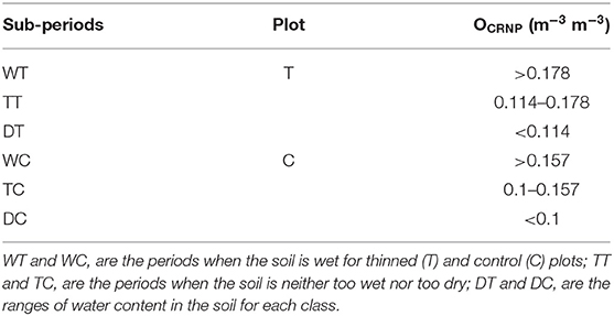
Table 2. Classification according to the water content in the soil.
Subsequently, Npihv(t) was obtained by multiplying Npih by a correction factor (fveg) calculated as follows (Equation 14):
Finally, when Npihv was obtained, the optimization of N0 was carried out again, to check for the variation of RMSE when using the vegetation correction factor (fveg).
Cosmic-Ray Neutron Probe Validation
The validation was carried out by comparing the CRNP and capacitance soil moisture estimations using two methodologies, the RMSE and the Kling-Gupta efficiency (KGE) (Gupta et al., 2009; Kling et al., 2012). This validation was independently developed for T and C plots, not only for the whole time series, but also for three different sub-periods. The semi-arid climate conditions of the study site are expected to provide soil moisture values within a wide range, which includes wet and very dry periods. Schreiner-McGraw et al. (2016) also studied the performance of CRNP in a semi-arid environment, and in spite of the good results, the worst performance was observed in wet and dry periods. Hence, with the aim to assess the CSR performance under very different soil moisture conditions, this study divides the soil moisture dataset according to the capacitance soil moisture values. This classification in sub-periods was done for each plot, by using the machine learning methodology K-Nearest Neighbor (kNN) (Cristianini and Shawe-Taylor, 2000; Chirici et al., 2016). As a result, three sub-groups (k = 3) per plot were obtained: wet (WT, WC), transition (TT, TC) and dry (DT, DC) (see Table 2).
The RMSE was calculated as the difference in soil moisture value measured by the capacitance method (Og) and the CRNP (OCRNP):
KGE uses the difference in the ratio between the modeled (OCRNP) and observed (Og) soil moisture values (β = OCRNP/Og) and the variability in their respective time series [γ = (σCRNP/μCRNP)/(σg/μg)]; where modeled values are those obtained as described in sections Cosmic-ray sensor neutrons correction and calibration and Considering the biomass effect with the CRNP, and the observed ones are the mean values from the capacitance probes for each experimental plot. KGE was obtained according to Equation (16), where r is the correlation coefficient between modeled and observed values.
KGE ranges between 0 and 1, and 1 indicates a perfect result. The CRNP effective depth of each probe was calculated according Franz et al. (2012).
Statistical Analyses
The assumption of a Gaussian distribution of the different datasets was studied using a Kolmogorov-Smirnov (K-S) test with the Lilliefors correction. To analyze the correlations between soil moisture (capacitance and CRNP) and the environmental variables, a Pearson correlation test was done for variables for which the null hypothesis that these variables are Gaussian distributed was not rejected. On the other hand, a Spearman non-parametric correlation test was done for the variables for which the null hypothesis that they are Gaussian distributed was rejected. Both tests, Pearson and Sperman, were carried out at p < 0.05 level. Subsequently, the temporal lag between O and the environmental variables was studied by daily misplacing the environmental variables until the time lag with the greatest correlation and significance was found.
Finally, the technique of boosted regression trees (BRT) was used to study the capability of each methodology to register a physiological response to thinning. The BRT study was carried out following the methodology proposed by Elith et al. (2008), using as dependent variable stand transpiration and grouping the rest of the environmental variables in order to describe their importance: atmosphere (T, VPD, RAD, Ws), precipitation (Pg, Pn) and finally soil moisture (OCRNP and Og).
Results
Environmental Conditions During the Study Period
The environmental variables showed a typical Mediterranean semi-arid climate with an average annual gross precipitation (Pg) over the measurement period of 304 mm, where 253 and 193 mm correspond to the net precipitation (Pn) for T and C plots, respectively. The average annual temperature was almost 15°C, with annual minimum and maximum daily averages of −1.3 and 30.3°C, and the annual average vapor pressure deficit is 0.97 kPa (see Table 3).
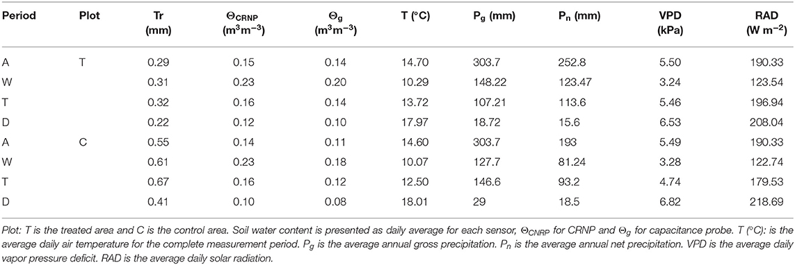
Table 3. Summary of environmental variables for the complete time series period (A) and when considering the three sub-periods according to the kNN classification (W, wet period; T, transition period; D, dry period).
The measurements of soil moisture with capacitance probes during the study period (January 2017- December 2019) were significantly different between C and T, where T showed higher values (p < 0.05; see Figure 3). Likewise, the complete time series of stand transpiration (Tr) showed significant differences between C and T plots (p < 0.05), with higher values now for the C-plot and mean transpiration values of 0.63 vs. 0.39 mm day−1 for C and T, respectively.
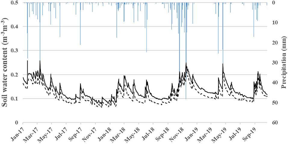
Figure 3. Soil water content measured with capacitance probes in each plot. Blue bars represent the daily gross precipitation. Black line is the soil water content measured with capacitance probes in T-Plot. Black dashed line is the soil water content measured with capacitance probes in C-Plot.
Soil Characteristics
Tables 4, 5 show soil characteristics of the experimental plots. Soil has a loamy-clay texture with a high content of stones and a well-developed organic horizon (litter layer) mainly composed by needles. The C plot shows a more extended and thicker litter layer than the T plot (see Table 5).
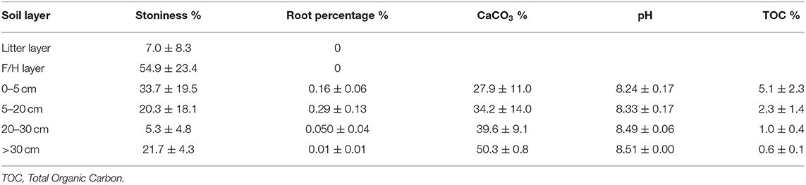
Table 4. Soil characteristics at the experimental plots.
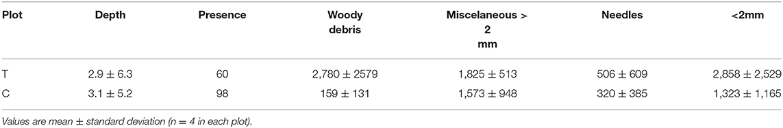
Table 5. Organic material (g m−2), depth (mm) and presence (%) of the litter layer in both experimental plots.
Calibration and Validation of the CRNP
Calibration for Both Plots
The calibration was carried out following Bogena et al. (2013), with and without applying the vegetation correction factor, fveg (see Table 6). The vegetation effect appears not to be significant in the T plot, where in spite of showing lower N0 and RMSE, no significant differences were observed when comparing the OCRNP values with and without the application of fveg. On the contrary, the fveg in the C plot did significantly decrease OCRNP measurements (mean OCRNP with and without fveg of 0.144 and 0.216 m−3m−3, respectively) (see Figure 4 and Table 6). The general validation of CRNP although showed a slight overestimation of O, resulted in KGE values of 0.84 and 0.40 for T and C plots, respectively, without applying the vegetation correction factor. When applying fveg, the performance was not affected for the T plot, but the KGE value of C increased to 0.75 (see Table 7 and Figure 5). Likewise, the validation for the 3 different sub-periods (wet, transition, and dry) showed only a significant effect of the vegetation correction factor for the control plot improving the performance (see Table 7).
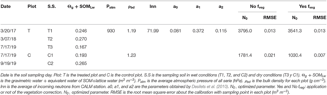
Table 6. Soil characteristics and variables for CRNP calibration.
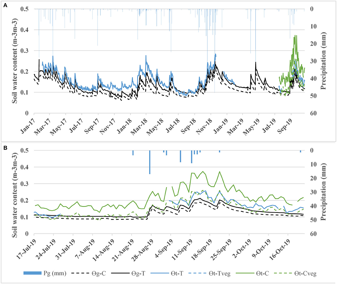
Figure 4. (A) Comparison of soil water content values measured using capacitance probes (Og−T and Og−C) and CRNP at the T and C plots with the application of the vegetation correction factor fveg (OCRNP−Tfveg and OCRNP−Cfveg) and without the application of the vegetation correction factor (OCRNP−T and OCRNP−C). (B) Zoom of date comparison between plots.
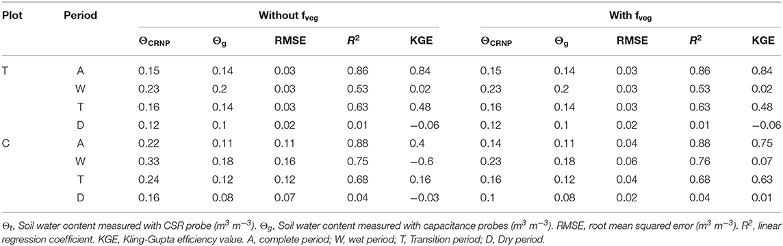
Table 7. Validation results of both CRNP probes.
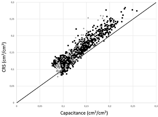
Figure 5. Comparison of soil water content values measured using capacitance and CRNP probes at the T (black squares) and C (gray circles) plots after the vegetation correction.
As expected, the partial validation using the different sub-periods provided the lowest CRNP measurement accuracy during extreme soil water conditions (dry and wet) at both plots, whereas the best performance was found during the transition period (see Table 6). Og at the different soil depths (15 cm, 30 cm and its averaged value) and ΘCRNP were significantly correlated, for both plots, and for the wet and transition sub-periods. However, for the dry sub-period, Og−C values did not show significant correlations. On the other hand, the effective depth of both CRNP ranged from 18.5 to 28.0 cm for T plot, and from 18.1 to 29.9 cm for C plot, indicating its suitability to be compared to Og at 15 and 30 cm depth.
Relationship Between Soil Moisture (EC-5 and CRNP), Environmental Variables, and Stand Transpiration
According to Table 8, the general pattern of correlation among Θ and environmental variables was quite similar for both measurement methods when considering the entire measurement period, although the CRNP showed stronger correlations with the environmental variables. Likewise, the temporal dynamics of the three different EC-5 sensors was very similar in both plots and during all periods and sub-periods (see Table 8).
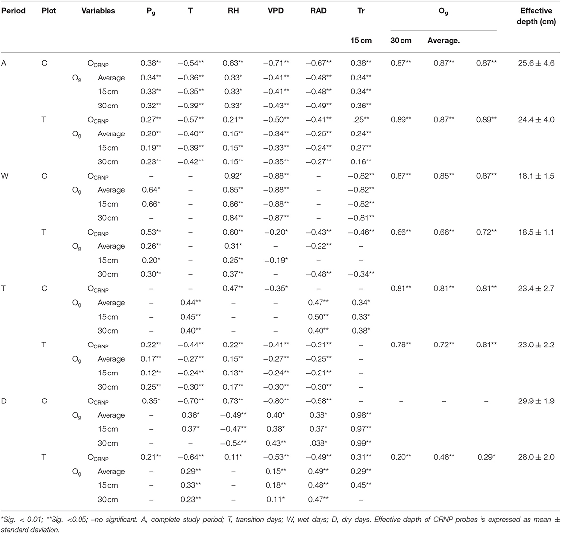
Table 8. Matrix of Spearman correlations among soil water content measured with capacitance (Og) and CSR (OCRNP) probes and the environmental variables at thinned (T) and control (C) plots: Average temperature (Tm), Gross precipitation (Pg), accumulated precipitation (Pac), vapor pressure deficit (VPD), radiation (RAD), and stand transpiration (Tr).
Correlations among O and the environmental variables varied between plots and sub-periods, but generally, T plot showed a better agreement between both methodologies than C plot. In this sense, OCRNP−T only behaved differently during the dry period, where it was significantly correlated to all the environmental variables, while Og−T was only correlated to air temperature, VPD, and RAD. On the contrary, OCRNP−C and Og−C, showed different relationships with the environmental variables during the three sub-periods (see Table 8).
CRNP measurements showed a significant correlation with RH and VPD at both plots and during all sub-periods, while EC-5 measurements were not always significantly related to these variables, and when they were, the sign of the correlation was not always the same. During the dry sub-period, CRNP for the control and thinning plots showed opposite relationships with RH (positive) and VPD (negative) than capacitance. Gross precipitation revealed a positive relationship with OCRNP−T during all sub-periods, while the relationship with OCRNP−C was only significant during the dry sub-period (see Table 8).
CRNP and EC-5 showed a positive relationship with Tr, if we consider the complete time series. It shows that higher soil moisture content is associated with higher transpiration. However, for the wet sub-period both soil moisture measurement techniques showed a negative correlation with transpiration. It seems that in the wet subperiod soil moisture availability is not a limitation for transpiration anymore. For the transition sub-period transpiration showed only a positive correlation with Og−C, and no significant correlations with Og−T, OCRNP−T, and OCRNP−C. The dry period also showed different behavior between measurement methods and plots. While OCRNP−C did not have a significant correlation with transpiration, Og−C was highly correlated to transpiration. On the contrary, OCRNP−T was positively correlated to Tr, and so were Og−T average at 15 cm, while 30 cm measures were negatively correlated to Tr (see Table 8).
Finally, the temporal lag of the correlation between O and the environmental variables, including transpiration at the C and T plots, was analyzed. According to this analysis, there was a differential behavior between plots and methodologies. The T plot showed similar temporal lags for both measurement techniques, while the C plot showed earlier responses of CRNP soil moisture to temperature, VPD and RH than soil moisture measured by capacitance probes. On the contrary, the response to cumulated precipitation (4 days) and solar radiation (1 day) was the same for the different plots and measurement techniques. No temporal lag of Tr nor RH was observed at T plot when using either CRNP or capacitance, while C plot showed a temporal lag of 1 day with Tr, and 0 and 1 day for RH with OCRNP−C and Og−C, respectively.
Importance of Thinning Application on Stand Transpiration
The previous results pointed to a similar performance of CRNP and EC-5, although CRNP was consistently more affected by the atmospheric variables than EC-5. However, concerning stand transpiration, the difference between the two measurement techniques was larger, mainly for the control plot. With the aim to analyze this difference, two transpiration models were studied considering either CRNP or EC-5 measurements by means of boosted regression trees (BRT). To this end, transpiration was used as a dependent variable to determine the importance of thinning, and two different transpiration models were generated, one with OCRNP values and another one with Og values as independent variables together with meteorological and rainfall partitioning variables. The BRT models showed different degrees of fitting (CRNP-model: cv-correlation = 0.96, R2 = 0.92; EC-5-model: cv-correlation = 0.97, R2 = 0.95) that indicated a good performance of both models. The relative importance of each variable is shown in Table 9. The results showed once again the similarity between both measurement techniques, although a slightly stronger correlation in the CRNP-model with atmospheric variables was confirmed, as the CRNP-model relied more on atmosphere and less on soil moisture and thinning than the EC-5-model.
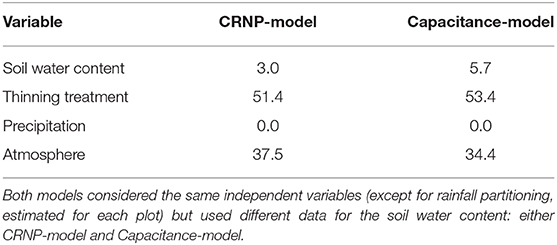
Table 9. Relative importance (%) of the different variables considered in the transpiration models using boosted regression trees.
Discussion
This study focused on the performance of CRNP for obtaining reliable soil moisture values in a semi-arid forest, and on the sensitivity of CRNP to forest management by comparing thinned and non-thinned forest experimental plots.
In general, calibration (RMSE: 0.013 and 0.007 m3 m−3 for T and C plots, respectively) and validation (KGE: 0.84 and 0.75 for T and C plots, respectively) procedures showed values that indicate a good performance of CRNP, which in the case of the non-thinned forest (C-plot), improved with the application of the vegetation correction factor. These values are comparable to those obtained in other studies such as that of Bogena et al. (2013); they obtained a RMSE value of 0.025 m3 m−3 for a forested area, and Li et al. (2019), who found a RMSE value of 0.025 m3 m−3 for a semi-arid environment, or Lv et al. (2014), who found RMSE values varying between 0.011 and 0.023 m3 m−3 for a humid forest (gross precipitation of 950 mm y−1). However, when comparing OCRNP to Og, there is a general overestimation by CRNP that can be attributed to the influence of biomass and the different measurement depths of both methodologies and changes under the different subperiods (Figure 5). In fact, a closer analysis by dividing the time series into O sub-periods revealed that this general performance decreases when dealing with extreme O values. In this sense, this study found the CRNP performed worst in both wet and dry sub-periods, where O was overestimated in both plots, and even reaching negative KGE values for the T plot. Schreiner-McGraw et al. (2016) studied the performance of CRNP in two semi-arid catchments and also obtained the worst results during dry and wet periods. As stated by these authors, the worst performance under extreme soil water conditions could indicate that OCRNP has a tendency to dry less quickly during some rainfall events, and therefore overestimate O values. Schreiner-McGraw et al. (2016) attributed this behavior to landscape features such as nearby channels and their associated zones of soil water convergence that remain wetter than areas measured by the distributed sensor network. However, in our case, there are no nearby channels, but a thick and continuous litter layer (Table 4) capable of retaining a significant amount of water, and probably increasing OCRNP values (Heidbüchel et al., 2016). In agreement with this, OCRNP values showed more and stronger correlations with the environmental variables, which probably indicate the effect of this litter layer, whose wetting-drying dynamics are more strongly related to precipitation than deeper soil layers (Bogena et al., 2013). During the dry sub-period, these relationships were even opposite to those of the capacitance sensor, and therefore closer to the faster wetting-drying dynamics of surface water (see Table 8).
The different measurement depths of the EC-5 sensors and CRNP could also explain this performance variation. The effective penetration depth of CRNP is dynamic, as it strongly depends on SWC, decreasing non-linearly from around 76 cm in dry soils to ~12 cm in saturated soils (Zreda et al., 2012). Our data showed an effective penetration depth between 18 and 30 cm. These values are very close to the location of the capacitance probes, and therefore, the correlations between OCRNP and Og at 15 and 30 cm depth might not be significantly different. Accordingly, when comparing these values (OCRNP and Og, at 15 and 30 cm depth), no clear differences were found between them. The CRNP is most sensitive to soil moisture within the first centimeters and this sensitivity decreases non-linearly with increasing depth (Schrön et al., 2017). Correspondingly, the shallower capacitance measurements (Og at 15 cm) always showed the strongest relationship with OCRNP (see Table 8), but the correlation with Og at 30 cm was also significant at both plots and during all sub-periods, except for the dry sub-period, where the behavior changes in both plots. During this period, the effective measurement depth of CRNP also reached its maximum value (28 cm), and in the case of the T plot, the correlation with Og at 30 cm was higher than that of at 15 cm. Regarding the C plot, despite the fact that the maximum of the CRNP effective penetration depth was also 30 cm, no significant correlations were found for any of the measurement depths. This fact could be attributed to the low Og values registered during this period (0.09 ± 0.004 m3 m−3), although this value was just slightly lower than that of T plot during the same sub-period, where the correlations were significant. Thus, the reason could not be the low soil moisture but difference in processes between the two plots. Looking closely to the comparison between both methodologies during this sub-period, OCRNP−T and OgT show a very similar variation, while on the contrary, in spite of the short measurement period, OCRNP−C shows a standard deviation (0.012 m3 m−3) one order of magnitude higher than OgC (0.004 m3 m−3). Schreiner-McGraw et al. (2016) and Heidbüchel et al. (2016) reported that the CRNP measurement signal is more strongly influenced by the first 5 soil cm depth, and Lv et al. (2014) reported a more sensitive response of CRNP to small rainfall events than soil moisture measured by TDR at 10 cm depth. Thus, soil water dynamics that CRNP is registering might probably correspond more to the upper 5–10 cm, including the litter layer, whose wetting-drying dynamics is significantly faster than that of deeper soil layers [see Bogena et al. (2013)].
When analyzing the performance of CRNP with and without forest management, a differential behavior of both plots was observed. In general, OCRNP from T plot adjusted better to Og values, and was not significantly affected by the vegetation correction factor. This is related to the low biomass present in the T plot (1.4 kg m−2). According to Hawdon et al. (2014), values lower than 5 kg m−2 may have little influence on the neutron count rate. Higher biomass also implies higher water interception, which also affects the neutron count and may cause an overestimation of soil moisture (Heidbüchel et al., 2016; Jakobi et al., 2018). The litter layer of the C plot is practically continuous and thicker than that for the T plot (Table 4), and may have a similar effect as rainfall interception, increasing the possibility of overestimating O after rainfall events. Hence, the better performance of CRNP-T could be attributed to the biomass effect (both, soil and vegetation), but also to spatial and temporal representativeness. As shown in Figure 1, the T plot includes most of CRNP horizontal footprint, whereas for the C-plot this is <50% (Schrön et al., 2017). Thus, since the C plot capacitance probes were installed only within this non-thinned area, comparing these values with those that include other conditions (CRNP-C) could undermine actual CRNP performance. In terms of temporal representativeness, the time series of the T plot was significantly longer than that of the C plot, which only covered the summer period. Furthermore, during this study period a high number of rainy days occurred with high soil moisture conditions in which, as seen before, the CRNP showed its worst performance. Therefore, the investigation period of the C plot may have been too short to adequately test the performance of the CRNP.
Despite the fact that the performance of the CRNP-C was worse than for CRNP-T, OCRNP−C values showed a higher correlation with environmental variables than OCRNP−T. This difference between the plots could be due to the influence of biomass on the fast neutron intensity (e.g., by rainfall interception of the vegetation or the litter layer), i.e., by hydrogen pools other than soil moisture (Heidbüchel et al., 2016). However, on the other hand, Og−C values were more correlated to environmental variables than Og−T. In this case, biomass may also be responsible of this difference, but in a different way. Soil moisture in semi-arid forests is an important water source for the vegetation development (Castillo et al., 2003; Seeger et al., 2004), and changes in this variable highly affect the forest dynamic. In the same way, changes in vegetation (thinning) affect rainfall partitioning and tree water consumption, which directly affects soil moisture. This effect of forest management has already been pointed out by del Campo et al. (2019b) for this study site, as the thinning had significantly influenced rainfall partitioning by reducing water interception and increasing soil moisture. Thus, this effect together with the significant decrease in tree water competition increases soil water availability and therefore decreases the dependence of soil moisture dynamics on environmental variables.
The stand transpiration also showed different correlations with soil moisture for the plots, and in this case the C-plot is the one that showed significant relationships with both OCRNP−T and Og−T, while in the T plot the correlations were weaker or non-significant, such as during the transition sub-period. Furthermore, in contrast to the environmental variables, the highest correlation values were found for Og−C in this case, probably due to the biomass influence on the CRNP and the different measurement support of the two methods both in terms of footprint and penetration depth. During the dry and transition sub-periods, OCRNP−C did not show significant correlations with transpiration, while Og−C values (at both measurement depths) were significantly correlated with transpiration. Probably, during these sub-periods, the trees were significantly transpiring more water from deeper soil layers, which would enhance the relationship with Og at 15–30 cm.
Furthermore, the differential behavior of both soil moisture measurement methods when comparing between plots is probably related to the significant effect of thinning on rainfall partitioning, as already observed by del Campo et al. (2019b). The increase of O together with the diminishing of tree water competition allows trees to transpire whenever the combination between water availability and atmospheric demand is present. This relationship is possibly due to the fragile equilibrium between water supply and demand that exists in semi-arid forests, where the water in the soil is what limits the transpiration (del Campo et al., 2014). Nevertheless, since O is higher in the T plot, the limiting role of the soil is significantly reduced, and therefore the tree water consumption would be more related to the atmospheric demand.
Conclusions
The results presented in this study confirmed the overall reliability of CRNP in obtaining soil moisture in semi-arid forests, but a lower measurement accuracy was found for very dry and wet conditions. Furthermore, our results also show the relevance of spatial heterogeneity within the measuring footprint to the CRNP measurements. Since the CRNP has a much larger measuring volume compared to capacitance sensors, this difference must be considered when comparing the two measurements. Furthermore, it has to be considered that in forests other processes, e.g., the interception of the litter layer or the vegetation, can influence the comparison with capacitance-based in-situ sensors. The CRNP showed stronger relationships with environmental variables (T, HR, VPD, and RAD), which were attributed to the effect of the soil litter layer together with the high sensitivity of the CRNP to the top 5–10 cm of soil. Both soil moisture measurement methods showed a similar correlation with tree transpiration, only insignificantly stronger for capacitance sensors. Both methods were affected by biomass management, although probably to different extents. The capacity sensors were directly affected by the increasing net precipitation following forest management, while the CRNP was also affected by precipitation interception, as this reduced neutron intensity leading to overestimation of soil moisture during rainfall and shortly afterwards. In either case, both methods were able to capture the physiological response of trees to thinning, which was reflected in the increase in the correlation between transpiration and soil moisture.
Data Availability Statement
The datasets presented in this article are not readily available because the data set is available under request, and its usage is condition to previous agreements such as paper authorship. Requests to access the datasets should be directed to María González-Sanchis, bWFjZ29uc2FAZ21haWwuY29t.
Author Contributions
MG-S analyzed the results and wrote the paper. JG-S calibrated the CRS and helped with to build the paper and with the analysis of the results. AM contributed writing the paper and analyzing the results. AL and IB did the soil sampling campaigns and analyzed the samples. ER worked with the raw data and did the first calibration approach. HB, and H-JH contributed with both CRS probes and usage and calibration support. AC is the coordinator of the whole project. All authors contributed to the article and approved the submitted version.
Funding
This study is a component of the research projects: E-HIDROMED (CGL2014-58127-C3) and CEHYRFO-MED (CGL2017-86839-C3-2-R) funded by the Spanish Ministry of Science and Innovation and FEDER funds, and LIFE17 CCA/ES/000063 RESILIENTFORESTS. AM is beneficiary of an APOSTD fellowship (APOSTD/2019/111) funded by the Generalitat Valenciana.
Conflict of Interest
The authors declare that the research was conducted in the absence of any commercial or financial relationships that could be construed as a potential conflict of interest.
Acknowledgments
The authors are grateful to TERENO funded by the Helmholtz Association and the Federal Ministry of Education and Research of Germany for providing the CRNP, the Valencia Regional Government (CMAAUV, Generalitat Valenciana), the VAERSA staff, the Natural Park staff and the communal authority of Serra for their support and allowing the use of the Natural Park experimental forest.
References
Andreasen, M., Jensen, K. H., Desilets, D., Franz, T. E., Zreda, M. G., and Bogena, H. R. (2017). Status and perspectives of the cosmic-ray neutron method for soil moisture estimation and other environmental science applications. Vadose Zone J. 16:86. doi: 10.2136/vzj2017.04.0086
Baatz, R., Bogena, H. R., Hendricks Franssen, H. J., Huisman, J. A., Montzka, C., and Vereecken, H. (2015). An empirical vegetation correction for soil water content quantification using cosmic ray probes. Water Resour. Res. 51, 2030–2046. doi: 10.1002/2014WR016443
Bell, D. M., Bradford, J. B., and Lauenroth, W. K. (2014). Mountain landscapes offer few opportunities for high-elevation tree species migration. Glob. Chang. Biol. 20, 1441–1451. doi: 10.1111/gcb.12504
Berdanier, A. B., Miniat, C. F., and Clark, J. S. (2016). Predictive models for radial sap flux variation in coniferous, diffuse-porous and ring-porous temperate trees. Tree Physiol. 36, 932–941. doi: 10.1093/treephys/tpw027
Bogena, H. R., Huisman, J. A., Baatz, R., Hendricks Franssen, H.-J., and Vereecken, H. (2013). Accuracy of the cosmic-ray soil water content probe in humid forest ecosystems: the worst case scenario: cosmic-ray probe in humid forested ecosystems. Water Resour. Res. 49, 5778–5791. doi: 10.1002/wrcr.20463
Bogena, H. R., Huisman, J. A., Güntner, A., Hübner, C., Kusche, J., and Jonard, F. (2015): Emerging methods for non-invasive sensing of soil moisture dynamics from field to catchment scale: a review. WIREs Water 2, 635–647. doi: 10.1002/wat2.1097.
Brown, P., and Wu, R. (2005). Climate and disturbance forcing of episodic tree recruitment in a southwestern ponderosa pine landscape. Ecology 86, 3030–3038. doi: 10.1890/05-0034
Burgess, S. S. O., Adams, M. A., Turner, N. C., Beverly, C. R., Ong, C. K., Khan, A. A. H., et al. (2001). An improved heat pulse method to measure low and reverse rates of sap flow in woody plants. Tree Physiol. 21, 589–598. doi: 10.1093/treephys/21.9.589
Castillo, V. M., Gomez-Plaza, A., and Martinez-Mena, M. (2003). The role of antecedent soil water content in the runoff response of semiarid catchments: a simulation approach. J. Hydrol. 284, 114–130. doi: 10.1016/S0022-1694(03)00264-6
Chirici, G., Mura, M., McInerney, D., Py, N., Tomppo, E. O., Waser, L. T., et al. (2016). A meta-analysis and review of the literature on the k-nearest neighbors technique for forestry applications that use remotely sensed data. Remote Sens. Environ. 176, 282–294. doi: 10.1016/j.rse.2016.02.001
Coops, C. N., Waring, R. H., and Law, B. E. (2005). Assessing the past and future distribution and productivity of ponderosa pine in the Pacific Northwest using a process model, 3-PG. Ecol. Modell. 183, 107–124. doi: 10.1016/j.ecolmodel.2004.08.002
Cristianini, N., and Shawe-Taylor, J. (2000). An Introduction to Support Vector Machines and Other Kernel-based Learning Methods, 1st Edn. New York, NY: Cambridge University Press.
del Campo, A. D., Fernandes, T. J. G., and Molina, A. J. (2014). Hydrology-oriented (adaptive) silviculture in a semiarid pine plantation: how much can be modified the water cycle through forest management? Eur. J. For. Res. 133, 879–894. doi: 10.1007/s10342-014-0805-7
del Campo, A. D., González-Sanchis, M., García-Prats, A., Ceacero, C. J., and Lull, C. (2019a). The impact of adaptive forest management on water fluxes and growth dynamics in a water-limited low-biomass oak coppice. Agric. Forest Meteorol. 264, 266–282. doi: 10.1016/j.agrformet.2018.10.016
del Campo, A. D., González-Sanchis, M., Lidón, A., Ceacero, C. J., and García-Prats, A. (2018). Rainfall partitioning after thinning in two low-biomass semiarid forests: impact of meteorological variables and forest structure on the effectiveness of water-oriented treatments. J. Hydrol. 565, 74–86. doi: 10.1016/j.jhydrol.2018.08.013
del Campo, A. D., González-Sanchis, M., Lidón, A., García-Prats, A., Lull, C., Bautista, I., et al. (2017). “Ecohydrological-based forest management in semi-arid climate,” in Ecosystem Services of Headwater Catchments (Cham: Springer), 45–57.
del Campo, A. D., González-Sanchis, M., Molina, A. J., García-Prats, A., Ceacero, C. J., and Bautista, I. (2019b). Effectiveness of water-oriented thinning in two semiarid forests: The redistribution of increased net rainfall into soil water, drainage and runoff. For. Ecol. Manage. 438, 163–175. doi: 10.1016/j.foreco.2019.02.020
Desilets, D., and Zreda, M. (2003). Spatial and temporal distribution of secondary cosmic-ray nucleon intensities and applications to in-situ cosmogenic dating. Earth Planet. Sci. Lett. 206, 21–42. doi: 10.1016/S0012-821X(02)01088-9
Desilets, D., Zreda, M., and Ferré, T. (2010). Nature's neutron probe: Land surface hydrology at an elusive scale with cosmic rays. Water Resour. Res. 46, 21–42. doi: 10.1029/2009WR008726
Detty, J. M., and McGuire, K. J. (2010). Threshold changes in storm runoff generation at a till-mantled headwater catchment: threshold changes in runoff generation. Water Resour. Res. 46, 1–15. doi: 10.1029/2009WR008102
Elith, J., Leathwick, J. R., and Hastie, T. (2008). A working guide to boosted regression trees. J. Anim. Ecol. 77, 802–813. doi: 10.1111/j.1365-2656.2008.01390.x
Flinn, K. M., and Marks, P. L. (2007). Agricultural legacies in forest environments: Tree communities, soil properties, and light availability. Ecol. Appl. 17, 452–463. doi: 10.1890/05-1963
Franz, T. E., Zreda, M., Rosolem, R., and Ferré, T. P. A. (2012). Field validation of a cosmic-ray neutron sensor using a distributed sensor network. Vadose Zone J. 11, 46–56. doi: 10.2136/vzj2012.0046
Gardner, C. M. K., Dean, T. J., and Cooper, J. D. (1998). Soil water content measurement with a high-frequency capacitance sensor. J. Agric. Eng. Res. 71, 395–403. doi: 10.1006/jaer.1998.0338
González-Sanchis, M., Ruiz-Pérez, G., Del Campo, A. D., Garcia-Prats, A., Francés, F., and Lull, C. (2019). Managing low productive forests at catchment scale: considering water, biomass and fire risk to achieve economic feasibility. J. Environ. Manage. 231, 653–665. doi: 10.1016/j.jenvman.2018.10.078
Gupta, H. V., Kling, H., Yilmaz, K. K., and Martinez, G. F. (2009). Decomposition of the mean squared error and NSE performance criteria: implications for improving hydrological modelling. J. Hydrol. 377, 80–91. doi: 10.1016/j.jhydrol.2009.08.003
Hawdon, A., McJannet, D., and Wallace, J. (2014). Calibration and correction procedures for cosmic-ray neutron soil moisture probes located across Australia. Water Resour. Res. 50, 5029–5043. doi: 10.1002/2013WR015138
Hawley, M.E., Jackson, T. J., and McCuen, R. H. (1983). Surface soil moisture variation on small agricultural watersheds. J. Hydrol. 62, 179–200. doi: 10.1016/0022-1694(83)90102-6
Heidbüchel, I., Güntner, A., and Blume, T. (2016). Use of cosmic-ray neutron sensors for soil moisture monitoring in forests. Hydrol. Earth Syst. Sci. 20, 1269–1288. doi: 10.5194/hess-20-1269-2016
Jakobi, J., Huisman, J. A., Vereecken, H., Diekkrüger, B., and Bogena, H. R. (2018). Cosmic-ray neutron sensing for simultaneous soil water content and biomass quantification in drought conditions. Water Resour. Res. 54, 7383–7402. doi: 10.1029/2018WR022692
Jana, R. B., Ershadi, A., and McCabe, M. (2016). Examining the relationship between intermediate-scale soil moisture and terrestrial evaporation within a semi-arid grassland. Hydrol. Earth Syst. Sci. 20, 3987–4004. doi: 10.5194/hess-2016-186
Kling, H., Fuchs, M., and Paulin, M. (2012). Runoff conditions in the upper danube basin under an ensemble of climate change scenarios. J. Hydrol. 424-425, 264–277. doi: 10.1016/j.jhydrol.2012.01.011
Li, D., Schrön, M., Köhli, M., Bogena, H., Weimar, J., Jiménez Bello, M. A., et al. (2019). Can drip irrigation be scheduled with cosmic-ray neutron sensing? Vadose Zone J. 18:190053. doi: 10.2136/vzj2019.05.0053
Lv, L., Franz, T. E., Robinson, D. A., and Jones, S. B. (2014). Measured and modeled soil moisture compared with cosmic-ray neutron probe estimates in a mixed forest. Vadose Zone J. 13, 1–13. doi: 10.2136/vzj2014.06.0077
MAPA (1994) Métodos Oficiales de Análisis de Suelos y Aguas. Madrid: Ministerio de Agricultura, Pesca y Alimentación.
Mast, J., Fule, P., Moore, M., Covington, W. , and Waltz, A. (1999). Restoration of presettlement age structure of an Arizona ponderosa pine forest. Ecol. Appl. 9, 228–239. doi: 10.1890/1051-0761(1999)0090228:ROPASO2.0.CO
McJannet, D., Franz, T., Hawdon, A., Boadle, D., Baker, B., Almeida, A., et al. (2014). Field testing of the universal calibration function for determination of soil moisture with cosmic-ray neutrons. Water Resour. Res. 50, 5235–5248. doi: 10.1002/2014WR015513
Molina, A. J., Latron, J., Rubio, C. M., Gallart, F., and Llorens, P. (2014). Spatio-temporal variability of soil water content on the local scale in a Mediterranean mountain area (Vallcebre, North Eastern Spain). How different spatio-temporal scales reflect mean soil water content. J. Hydrol. 516, 182–192. doi: 10.1016/j.jhydrol.2014.01.040
Nelson, D. W., and Sommers, L. E. (1982). “Total carbon, organic carbon and organic matter,” in Methods of Soil Analysis. Part 2. Chemical and Mineralogical Properties (Madison: American Society of Agronomy), 539–579.
Rehfeldt, G., Jaquish, B., Saenz-Romero, C., Joyce, D., Leites, L., St Clair, J., et al. (2014). Comparative genetic responses to climate in the varieties of Pinus ponderosa and Pseudotsuga menziesii: reforestation. For. Ecol. Manage. 324, 147–157. doi: 10.1016/j.foreco.2014.02.040
Rodríguez-Iturbe, I., and Porporato, A. (2007). Ecohydrology of Water-Controlled Ecosystems: Soil Moisture and Plant Dynamics. Cambridge: Cambridge University Press
Rosolem, R., Hoar, T., Arellano, A., Anderson, J. L., Shuttleworth, W. J., Zeng, X., et al. (2014). Translating aboveground cosmic-ray neutron intensity to high-frequency soil moisture profiles at sub-kilometer scale. Hydrol. Earth Syst. Sci. 18, 4363–4379. doi: 10.5194/hess-18-4363-2014
Ruiz-Peinado, R., del Rio, M., and Montero, G. (2011). New models for estimating the carbon sink capacity of Spanish softwood species. Forest Syst. 20, 176–188. doi: 10.5424/fs/2011201-11643
Savage, M., Brown, P., and Feddema, J. (1996). The role of climate in a pine forest regeneration pulse in the southwestern United States. Ecoscience 3, 310–318. doi: 10.1080/11956860.1996.11682348
Schreiner-McGraw, A. P., Vivoni, E. R., Mascaro, G., and Franz, T. E. (2016). Closing the water balance with cosmic-ray soil moisture measurements and assessing their relation to evapotranspiration in two semiarid watersheds. Hydrol. Earth Syst. Sci. 20, 329–345. doi: 10.5194/hess-20-329-2016
Schrön, M., Köhli, M., Scheiffele, L., Iwema, J., Bogena, H. R., Lv, L., et al. (2017). Improving calibration and validation of cosmic-ray neutron sensors in the light of spatial sensitivity. Hydrol. Earth Syst. Sci. 21, 5009–5030. doi: 10.5194/hess-21-5009-2017
Seeger, M., Errea, M. P., Begueria, S., Arnáez, J., Mart, I. C., and Garcia-Ruiz, J. M. (2004). Catchment soil moisture and rainfall characteristics as determinant factors for discharge/suspended sediment hysteretic loops in a small headwater catchment in the Spanish Pyrenees. J. Hydrol. 288, 299–311. doi: 10.1016/j.jhydrol.2003.10.012
Seyfried, M. S., and Murdock, M. D. (2001). Response of a new soil water sensor to variable soil, water content, and temperature. Soil Sci. Soc. Am. J. 65, 28–34. doi: 10.2136/sssaj2001.65128x
Topp, G. C., and Ferré, T. P. (2006). “Measuring soil water content,” in En Encyclopedia of Hydrological Sciences Vol. 2, ed M. G. Anderson (Chichester: Wiley). p. 1077–1088.
van Mantgem, P. J., Stephenson, N. L., Byrne, J. C., Daniels, L. D., Franklin, J. F., Fulé, P. Z., et al. (2009). Widespread increase of tree mortality rates in the western United States. Science 323, 521–524. doi: 10.1126/science.1165000
Vereecken, H., Huisman, J. A., Bogena, H. R., Vanderborght, J., Vrugt, J. A., and Hopmans, J. W. (2008). On the value of soil moisture measurements in vadose zone hydrology. A review. Water Resour. Res. 44:W00D06. doi: 10.1029/2008WR006829
Wang, E., Smith, C. J., Macdonald, B. C., Hunt, J. R., Xing, H., Denmead, O. T., et al. (2018). Making sense of cosmic-ray soil moisture measurements and eddy covariance data with regard to crop water use and field water balance. Agr. Water Manag. 204, 271–280. doi: 10.1016/j.agwat.2018.04.017
Williams, A. P., Allen, C. D., Macalady, A. K., Griffin, D., Woodhouse, C. A., Meko, D. M., et al. (2013). Temperature as a potent driver of regional forest drought stress and tree mortality. Nat. Clim. Change 3, 292–297. doi: 10.1038/nclimate1693
Zreda, M., Desilets, D., Ferré, T. P. A., and Scott, R. L. (2008). Measuring soil moisture content non-invasively at intermediate spatial scale using cosmic-ray neutrons. Geophys. Res. Lett. 35:L21402. doi: 10.1029/2008GL035655
Keywords: forest hydrology, silviculture, capacitance sensors, cosmic-ray sensor, Pinus halepensis
Citation: González-Sanchis M, García-Soro JM, Molina AJ, Lidón AL, Bautista I, Rouzic E, Bogena HR, Hendricks Franssen H-J and del Campo AD (2020) Comparison of Soil Water Estimates From Cosmic-Ray Neutron and Capacity Sensors in a Semi-arid Pine Forest: Which Is Able to Better Assess the Role of Environmental Conditions and Thinning? Front. Water 2:552508. doi: 10.3389/frwa.2020.552508
Received: 16 April 2020; Accepted: 29 September 2020;
Published: 17 November 2020.
Edited by:
Bhavna Arora, Lawrence Berkeley National Laboratory, United StatesReviewed by:
Tim Scheibe, Pacific Northwest National Laboratory (DOE), United StatesRaghavendra Belur Jana, Skolkovo Institute of Science and Technology, Russia
Copyright © 2020 González-Sanchis, García-Soro, Molina, Lidón, Bautista, Rouzic, Bogena, Hendricks Franssen and del Campo. This is an open-access article distributed under the terms of the Creative Commons Attribution License (CC BY). The use, distribution or reproduction in other forums is permitted, provided the original author(s) and the copyright owner(s) are credited and that the original publication in this journal is cited, in accordance with accepted academic practice. No use, distribution or reproduction is permitted which does not comply with these terms.
*Correspondence: María González-Sanchis, bWFjZ29uc2FAZ21haWwuY29t