 Guillaume Coiffier
 Philippe Renard
 Sylvain Lefebvre3
- 1Centre for Hydrogeology and Geothermics, École Normale Supérieure de Lyon, Lyon, France
- 2Computer Science Department, University of Neuchâtel, Neuchâtel, Switzerland
- 3Université de Lorraine, CNRS, INRIA, Loria, France
Generative Adversarial Networks (GAN) are becoming an alternative to Multiple-point Statistics (MPS) techniques to generate stochastic fields from training images. But a difficulty for all the training image based techniques (including GAN and MPS) is to generate 3D fields when only 2D training data sets are available. In this paper, we introduce a novel approach called Dimension Augmenter GAN (DiAGAN) enabling GANs to generate 3D fields from 2D examples. The method is simple to implement and is based on the introduction of a random cut sampling step between the generator and the discriminator of a standard GAN. Numerical experiments show that the proposed approach provides an efficient solution to this long lasting problem.
1. Introduction
For a wide range of problems in the hydrological sciences, there is a need to employ stochastic models to generate spatial fields. These fields can represent for example climatic data, or physical parameters of the atmosphere, ground or underground.
In that framework, multiple-points statistics and the concept of training image became very popular in the last 10 years (Journel and Zhang, 2006; Hu and Chugunova, 2008; Mariethoz and Caers, 2014; Linde et al., 2015). The key idea in these approaches is to use an exhaustively mapped example (the training image) of the type of spatial patterns that are expected to occur for a given variable and at a given scale. The training image is then used to train a spatial statistics non-parametric model. The main advantage of that approach is that it allows to transfer information about spatial patterns coming from external information such as an analog site or data set to constrain the stochastic model. The range of applications is very broad and includes subsurface hydrophysical parameters (Mariethoz et al., 2010; Barfod et al., 2018), rainfall simulation (Oriani et al., 2014), bedrock topography below glaciers (Zuo et al., 2020), soil properties (Meerschman et al., 2014), landforms attributes (Vannametee et al., 2014), etc.
More recently, Deep Learning algorithms and especially Generative Adversarial Networks (GAN) (Goodfellow et al., 2014) have sparked a very strong interest thanks to their ability to generate stochastic fields showing a high degree of similarity with the training data sets (Chan and Elsheikh, 2017; Mosser et al., 2017a,b; Laloy et al., 2018). While this is very similar in principle to Multiple Point Statistics (MPS), a key feature of GAN is that they can be trained to represent a mapping from a low dimensional space to the manifold that supports the training data set. This feature allows GAN to represent complex fields via a low dimension vector of continuous values. Such a parametrization can then be used for example in the context of inverse modeling (Laloy et al., 2018). Although they need a long training time, GAN also appear to be usually faster than previous MPS methods at generating a set of realizations.
When applied to underground hydrology, and especially for uncertainty analysis or to solve inverse problems, a difficulty with the MPS or GAN approaches is to obtain 3D training images or examples. In practice, it is often very difficult, if not impossible, to collect exhaustive and accurate data about the three dimensional distribution of rock types (or physical properties) at depth. To circumvent that problem, in many applications, the 3D training images are derived from other types of models such as object based or process based models (de Marsily et al., 2005). But this is not always satisfying because the object based models imply additional assumptions and are not directly based on data when these are available in 2D.
Indeed, many two-dimensional data sets are available. They are much easier to collect than the 3D data sets using for example: remote sensing techniques, direct observation on outcrops, or microscopic data acquisition on thin sections of rocks. Furthermore, geologists are used to draw conceptual cross sections of typical structures. Therefore, simulating 3D stochastic fields from 2D examples is of high practical importance, and different techniques have been developed to solve that problem. In the framework of MPS, the approaches are often based on probability aggregation techniques or use some successive 2D simulation techniques (Okabe and Blunt, 2007; Comunian et al., 2012; Kessler et al., 2013; Cordua et al., 2016; Chen et al., 2018). In rock physics, the simulation of 3D porous media from 2D sections has been addressed in numerous articles (e.g., Adler et al., 1990; Yeong and Torquato, 1998; Karsanina and Gerke, 2018). Simulated annealing is often used in this context and allows to generate random fields which reproduce specific morphological features such as correlation functions or connectivity curves derived from the 2D data sets (e.g., Gerke and Karsanina, 2015; Lemmens et al., 2019). Deep Learning techniques have been used to accelerate MPS simulations in this framework (Feng et al., 2018). The 3D synthesis of textures from 2D examples has also been a main research topic in the field of computer graphics as shown in the review paper of Wei et al. (2009). These optimization methods achieve good results in the unstructured or weakly structured cases, but fail to capture long-range correlations. Works around GANs aiming at inferring a fixed 3D structured shape out of 2D projections has also been conducted (Gadelha et al., 2017, 2019), demonstrating the ability of these algorithms to infer an approximation of the three-dimensionnal shape of a deterministic object (like a plane or chair) out of a set of 2D views from a 3D scene. Here our problem is slightly different since we aim at inferring the statistical distribution of stochastic geological structures, which can have long range correlations, from a limited set of cross-sections through the domain.
In this paper, we introduce a novel approach based on GAN, called Dimension Augmenter GAN (DiAGAN). It allows to generate 3D fields from 2D training images, with sufficient resemblance and variability for geostatistical applications. The paper introduces first the general principle of GAN, then it describes the DiAGAN approach and illustrates it with a few examples.
2. Methodology
2.1. Generative Adversarial Networks
In the broadest sense, Machine Learning consists of designing algorithms that automatically find complex mappings from a given input data set to a given target data set . In practice, is often infinite and intractable, and we only have access to a finite set of training examples with their associated mapped values . Training algorithms then aim at finding the parametrized function fω that minimizes a loss function defined over :
with the hope of also minimizing the loss over , which would lead to good performances on new unknown data.
In Deep Learning more specifically, the parameterized function fω takes the form of a deep neural network: a structure made of an alternation of parameterized linear transformations called layers and non-linear component-wise activation functions. Neural networks are designed to be differentiable, so that their parameters can be optimized (trained) through gradient descent algorithms. Deep neural networks in their various forms had a deep impact in many domains in computer science with state of the art performance, including image recognition, natural language processing, data classification or artificial intelligence.
Technically, as long as a correct loss function is defined, that is to say a function that is differentiable and reaches an optimum when the desired mapping is achieved, any transformation from to can be learned, provided enough training examples in are given. In the context of procedural image synthesis, one difficulty is to define a loss function that assesses the quality of the generated samples in relation to the training image. Classical distances on the space of images, like the pixel-wise L2 norm indeed fail to capture the notion of resemblance between two images (note that in the following text we use the word image both for standard 2D images and 3D grids made of voxels). One has to define a loss function that takes into account multi-scale features and must be robust for instance to the fact that certain geological objects or patterns can be placed anywhere in the image, as their shape and frequency needs to be similar with the training image while their location is not fixed.
Generative Adversarial Networks (GAN) are a family of Deep Learning algorithms designed to tackle this problem. One of the key ideas here is that comparing two images can be done using a neural network fω that takes an image x as an input, and computes a numerical score fω(x) such that the higher the score, the more confident the network is of being fed with an image from the dataset it was trained with. Such a network fω, called a critic, can be plugged on the output of an image generator gθ, in order to give relevant numerical feedback.
More formally, the problem of image synthesis is the following. Given the set of all possible images of a certain size, we have access to a finite subset of training images (TI) . We suppose that images from were sampled from a probability distribution ℙdata over . From there, the goal is to be able to sample any image following the same probability distribution ℙdata. Because neural networks are essentially mappings, this is reduced in the case of GANs to finding a mapping from a latent space with a known distribution ℙz to the support space of ℙdata, under the constraint that ℙθ = gθ(ℙz) is as close as possible from ℙdata. Since ℙdata and ℙθ are intractable and can only be sampled from, the generator gθ and the critic fω have to be trained simultaneously in an adversarial fashion. Intuitively, one can see this process as if on the one hand, the generator tries to fool the critic by minimizing the distance between generated examples and real training examples. On the other hand, the critic is trained to separate training images from fake ones, thus maximizing the distance between ℙθ and ℙdata.
In the original GAN algorithm, Goodfellow et al. (2014) considered the Kullback-Leibler (KL) divergence as a distance between probability distributions. We chose to follow more recent works using the Wasserstein-1 distance, or Earth-mover (EM) distance (Arjovsky et al., 2017; Gulrajani et al., 2017), in an algorithm called the Wasserstein GAN (WGAN). This ultimately lead us to a two player zero-sum game using the following objective function (Gulrajani et al., 2017):
Equation (1) is directly used as a loss function during the training phase of a WGAN, during which theoretical expectations of probability distributions are replaced by statistical means over sampled examples. From the generator's point of view, the parameters are optimized to minimize −𝔼z~ℙz[fω(gθ(z))], while the critic's parameters are optimized with relation to the whole expression. In other words, gθ is trained to obtain the greatest possible score from the critic, whereas the critic optimizes both terms of Equation (1). The first term boils down to maximizing the EM distance between TIs, which are associated to high values of score, and generated images, associated to low values. However, this expression of the EM distance term only holds for fω being a Lipschitz function. The second term, called gradient penalty, proposed by Gulrajani et al. (2017), is a way to enforce this constraint on fω. In Equation (1), is a mix of ℙθ and ℙdata. More specifically, means that the variable was sampled from the distribution εℙdata + (1 − ε) ℙθ with ε being uniformly chosen in [0;1].
For the noise distribution ℙz, we consider vectors of ℝd where each coordinate is sampled independently from a standard normal distribution. Given the parameters of the generator, such a latent vector contains the whole information about the generated image, thus offering a compact representation. For generating images of size 64x64x64, we determined experimentally that d=256 was sufficient to represent the whole distribution.
2.2. From 2D to 3D
Going from 2D training examples to 3D realizations with a GAN is not straightforward, as the dimensionality of generated and training images should match in order for them to be fed to the same critic network. Most GAN algorithms directly feed the generated image inside the critic, but we propose to add an intermediate step to transform generated images, in order for them to match the TIs. Our training data consists of a set of triplets (Cx,Cy,Cz), where Ci is a two-dimensional image representing a typical cut perpendicular to axis i. The generator aims at generating 3D images which cuts along axis i resembles Ci. Note that the cuts are provided as independent images. They are not crossing each other at specific locations and they may not be completely compatible as will discuss in one of the examples.
To make the critic compare cuts, we incorporated a random cut sampler between the generator and the critic (Figure 1). This sampler extracts from a 3D generated example a triple of cuts (,,), with being chosen uniformly among all possible cuts along the corresponding axis. The discriminator then proceeds in comparing the patterns in the two triplets of cuts. The comparison is done for each direction but it does not account for the compatibility of the patterns along the intersection of the cuts since this information is not available in the training data. Depending on the type of symmetry and on available data, a similar technique can be used to account for one single set of cuts when the 3D patterns display similar structures along the x, y, and z directions, or instead a set of cuts along two axis when examples are available only along these two directions.
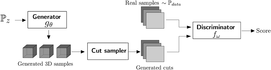
Figure 1. The overall organization of DiAGAN.
The sampler select the positions of the cuts randomly in a uniform distribution along each axis of the 3D domain, with only one cut per dimension. This mean that most of a generated image in the 3D domain will not be fed into the critic. However, since this sampling is random and thanks to the continuity of the GAN, this strategy proved to be rather efficient as we will illustrate with a few examples. Other approaches that may involve additional computations can be envisioned, this will be discussed in section 4.
In summary, the whole approach is stochastic and assumes that the 2D images that have been given in input can represent a cut anywhere in the domain. DiAGAN aims at reproducing these patterns in a stochastic manner, and assuming a spatial stationarity of the statistical process. In particular, it will not check precisely and in a deterministic manner the compatibility of the cuts at their intersection.
2.3. Neural Network Architecture
Following architectures proposed by Radford et al. (2015), we use convolutional neural networks for both our generator and critic. Throughout our experiments, we determined that precise architecture tuning was not necessary to get satisfactory results, as the WGAN is quite robust to those kind of hyperparameters. The main principles we used was to alternate convolutionnal layers, eventually normalization and upscaling, and non-linear activation.
Training images are normalized so that their values lay in [0;1]. Latent vectors z are sampled from a normal distribution of zero mean and standard deviation of 0.5. z is then reshaped into a 3-dimensional tensor that is fed into the convolutions. One can use regular convolution coupled with an upscaling function (like a trilinear interpolation), or a transposed convolution with a stride parameter greater than 1. The number of convolutional feature maps is decreasing with the depth, being divided by two at each layer.
We use the ReLU activation function (x ↦ max(0, x)) for every internal layers, and a sigmoid x ↦ 1/(1 + exp(−x)) for the final activation, in order to project the values back in the interval [0;1]. Alternatively, one could consider a normalization in [-1;1], Leaky ReLU function of parameter α=0.2 (x ↦ ReLU(x) − αReLU(−x)), and an hyberbolic tangent as the final activation.
The discriminator is composed of convolutional layers with 2D kernels. After the cut sampling step, we are left with 3 images of size NxN stacked into a 1xNx3N tensor, or a 3xNxN. 2D convolutions are applied to this tensor, alternating with max pooling operations. This halves the size of the tensor while the number of feature maps in the convolution is doubled. Alternatively again, one could replace the poolings by strides in the convolution. Activation functions are also ReLU of Leaky ReLU. At the end, a global max pooling operation is applied, to retrieve one numerical value for each feature map. The obtained vector of features is aggregated into a single numerical value by a dense layer.
We use instance normalization layers (Ulyanov et al., 2016) or batch normalization (Ioffe and Szegedy, 2015) after each convolution to guarantee the stability of the computation. The two methods performed equally well. Those normalization layers are present in the generator before each activation layers, but not in the critic, as they mess with the gradient penalty term (Gulrajani et al., 2017).
Table 1 summarizes the architecture of the convolutional networks that we use for DiAGAN. But note that the overall method is pretty robust, we tested several other architectures that worked also reasonably well. We expect that many other architectures could give good results.
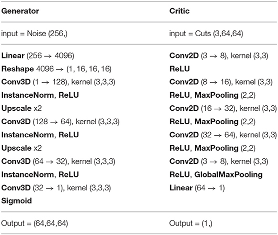
Table 1. Basic architecture used for DiAGAN with images of size 64 × 64 × 64 and a normalization of the TIs in [0;1].
Both generator and discriminator were trained using the Adam optimizer (Kingma and Ba, 2014) with a learning rate of 10−3, β1 = 0.5, and β2 = 0.9.
2.4. Quantitative Analysis of the Results
To assess the quality of the results, and compare the simulation with the reference when it is possible, we compute the indicator variograms and connectivity functions, as well as the Frechet Inception Distance (FID) between generated and real examples.
The indicator variogram γ(h) is defined as follows.
with I(x) being the indicator function of the facies 1. Since the cases that we investigate in this paper are binary, the indicator variogram is identical for facies 1 and 0.
The connectivity functions τi(h) describes the probability that two pixels located at a distance h belong to the same connected component, knowing that the first pixel is within the facies i.
τi(h) is computed for facies 0 and 1 separately. The connectivity functions are known to be different when computed on 3D or 2D fields. Indeed, the probability of having a connection between two points is generally higher in 3D for the same type of statistical configurations because the number of possible paths between the two points is larger in 3D. In the following of the paper, we compute the connectivity functions in 3D when we have a 3D reference. When the reference contained only 2D sections, we compare the connectivity functions computed only on 2D sections.
For the indicator variogram and the connectivity functions, we will compare the curves computed on individual realizations belonging either to the training set and to the set of simulations. The simulations are stochastic and therefore there will be some variability between these curves. To ease the comparison, we plot the mean values (as a function of distance) for the training sets and simulated sets. Because the number of simulations is limited (as well as the number of training examples), these mean curves are subject to estimation errors (standard error on the mean). Similarly to visualize the range of variations of the curves, we use the standard deviation of the curves computed on the reference set and superpose individual curves for the simulations. The standard deviation estimated on the reference is subject to an approximation error as well. These errors are not displayed on the graphs for the sake of visibility, but they have been studied for the first three cases.
The Frechet Inception Distance (FID), introduced by Heusel et al. (2017), is a heuristic measure of the distance between the distributions of generated sample and training images. Training image samples x and generated samples are fed into an InceptionV3 neural network (Salimans et al., 2016) trained for a classification task on the ImageNet dataset. This network outputs feature vectors y and ŷ. Denoting by (m, C) [resp. ()] the mean vector and covariance matrix over the samples y (resp. ŷ), the FID score is then defined as:
In DiAGAN, the FID gives an insight on the convergence and the relative quality of generated samples.
The variograms and connectivity functions, γ(h), τ(h) and the FID are computed and plotted along the three main directions X, Y, and Z.
3. Results
DiAGAN is implemented in both Pytorch and Tensorflow, two of the most popular Deep Learning librairies in Python. Both implementation lead to similar results.
3.1. Data Sets
To illustrate the proposed methodology, we consider six examples. The training images are shown in Figure 2. In all those examples, we consider only binary cases even if the method can be applied to discrete problems with more lithologies or even continuous problems. Outputs of our GANs, that are intrinsically continuous are thresholded to obtain binary data. Voxels with positive values are set to facies 1, while voxels 0 stay the same. Note that for most of the data sets the grid used for the simulation domain is smaller than the size of the training data sets. Therefore the size of the objects may look different when comparing a simulation with the training data visually.
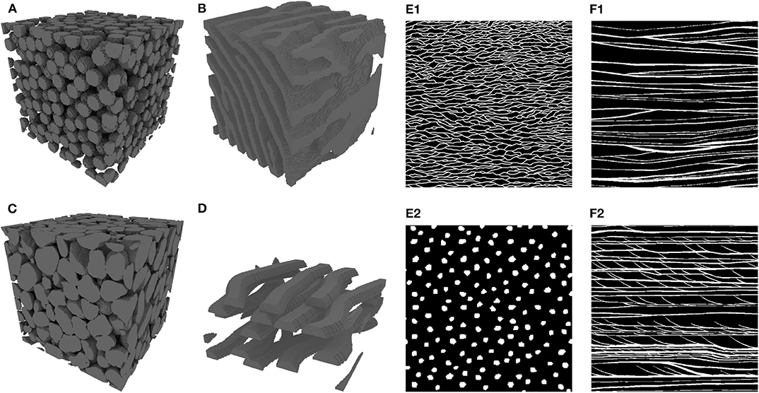
Figure 2. The six training data sets used in this study. Training images (A–D) are 3D examples fed as cuts, while TI (E) and (F) are cuts with no 3D ground truth. Details about the dimensions of the data sets and the data sources are given in the text. In all these data sets, the facies 0 is represented either in black or transparent, the facies 1 is represented either in gray for the 3D blocks and in white for the 2D images.
In general, a GAN requires a large training data set. However, in most applications in geosciences only a few training images are available or can be drawn manually by a geologist. Insufficient variability in the training data set prevents a GAN to train correctly. To tackle this problem, we use here large input images that were sub-sampled to generate a large number of smaller images. This fits our context well, since the challenge we seek to resolve is to synthesize plausible volume data from 2D inputs.
The datasets used in this paper are of two types.
On the one hand, three-dimensionnal data sets are represented in Figures 2A–D. They are used to test the method and allow to make a visual and quantitative comparison between the known 3D structure and the simulations obtained by our procedure using only 2D cuts through these volumes as training data.
• Figure 2A is a procedurally generated set of packed spheres. The grid has a size of 300 × 300 × 300 voxels. The spheres have diameters taken from a uniform distribution between 8 and 12 pixels and do not intersect each other. The global proportion of voxels occupied by the spheres is around 20%. This synthetic data set constitutes a benchmark even if it is far from a real-life geological application.
• Figure 2B is taken from the literature (Mariethoz and Kelly, 2011), it shows a stack of folded geological layers that were generated using an MPS method based on invariant distances and a rotation field1. The grid has a size of 126 × 126 × 120 voxels.
• Figure 2C is a rendering of a CT scan of the sandpack F42A obtained from Imperial College, London2. The grid has a size of 300 × 300 × 300 voxels.
• Finally, Figure 2D represents a geological reservoir at a kilometer scale that contains a set of fluvial channels. The image has been generated for this paper using the Tetris object based algorithm implemented in Ar2GEMS (Boucher et al., 2010). The grid has a size of 126 × 126 × 64 voxels.
On the other hand, training images depicted in Figures 2E,F are purely two dimensional. Assessing the quality of the output for these examples is more difficult because the 3D ground truth is not available and may not even exist. However, these cases are important to demonstrates the generalization capabilities of DiAGAN.
• The training image displayed in Figure 2E1 was taken from Laloy et al. (2018). It has a size of 1,000 × 1,000 pixels. This image was inspired by the training image of 2D channels created and used by Strebelle (2002) and extended by Laloy et al. (2018) to improve the diversity of the data set during the training phase. Since the original image has been heavily used as a benchmark in the MPS literature, we will refer to it as the Strebellian channels. It represents a map view of channel and matrix oriented along the (X, Y) and (X, Z) planes. The image displayed in Figure 2E2 was created manually for this paper and used to represent a vertical cross section along the (Y, Z) plane displaying roughly circular objects sections through the channels. It has a size of 600 × 746 pixels. With these two training images as input data, the aim is to simulate 3D channels or conduits propagating along the X direction. We took great care to ensure matching scales along the two images.
• Finally, Figures 2F1,F2 correspond to two perpendicular vertical sections (of about 30 × 30m) that have been mapped by Huysmans and Dassargues (2011) through the Brussels sand deposit. Both images have a size of 600 × 600 pixels. These data were used previously in Comunian et al. (2012). Image (f1) is a cut perpendicular to the X axis and (f2) is perpendicular to the Y axis. The horizontal cut is not available in that case. Notice how the two images differ: while layers perpendicular to the X axis are roughly horizontal and loosely connected, the one perpendicular to the Y axis presents some cross-bedding.
3.2. Realizations From 3D Datasets
DiAGAN has been first applied to generate 3D volumes of 64 × 64 × 64 voxels from sections taken inside the 3D examples. In real practical cases, these full 3D data sets would not be available. The aim here is to test the methodology in a situation where the 3D structure is known and can be used as a reference. While only 2D data taken from the 3D structure are used for training, the analysis of the resulting 3D simulation is compared to the original 3D data sets allowing to check if the simulation was correct. In particular, variograms and connectivity functions are computed in 3D.
The training times for these cases take from a few hours to a whole day on a rather old Tesla K40C GPU with 12 Gb of RAM. Once done, the generator is able to produce a simulation in less than a second.
Figure 3 a shows the evolution of the FID score during the training phase for the simulation of the 3D random packing of spheres. The FID score is dropping rapidly in the initial phase of training. This evolution is demonstrating the convergence of the method.
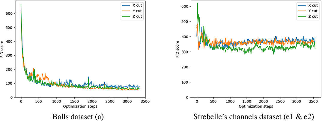
Figure 3. Evolution of the Frechet Inception Distance during training for two datasets. The FID score in approximated using 100 samples for both the TI and the generated images. A random cut along axes X, Y, and Z was taken from each samples to be fed inside the InceptionV3 model.
Figures 4, 5 show that the simulations of the spheres and sand grains display the correct order of magnitudes for the size of the objects as compared to the 3D references. The variograms and connectivity functions are reasonably well-reproduced. The trends are correct even if some minor differences are visible for example between the mean curves for the variograms. The computation of the standard error on the mean values for these curves show that the difference is not due to statistical variations but to slight differences between the set of simulations generated with DiAGAN and the set of training data resulting from some model errors. The same remark holds for the connectivity curves.
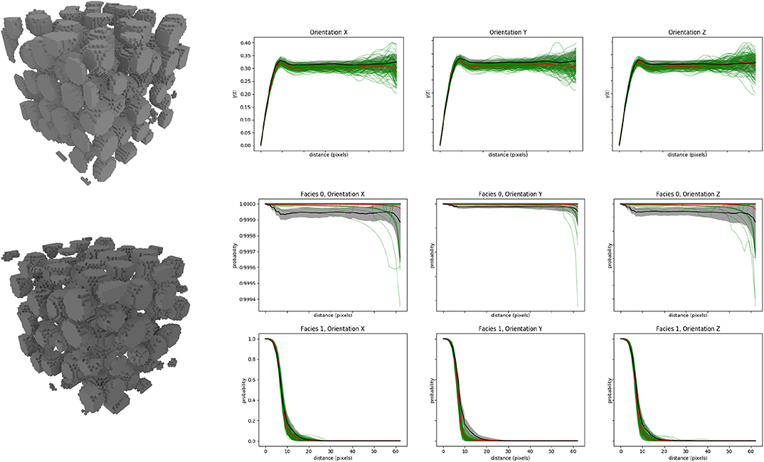
Figure 4. Results of DiAGAN on the ball dataset (a). Note for the visual comparison that the simulated domain has a size of 64x64x64 voxels while the training data set covers a larger area. The three upper curves present the variogram of 100 DiAGAN realizations (green) and their mean (red) along the three axis. The black curve is the mean of observations in the TI for samples of the same size, while the gray area is this mean plus or minus the observed standard deviation. Middle and bottom curves present the connectivity curve of the two facies of the image along the three axes, with the same color conventions.
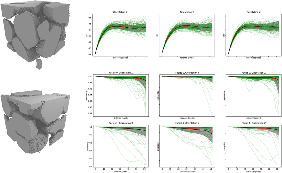
Figure 5. Results of DiAGAN on the sand grain dataset (c). Note for the visual comparison that the simulated domain has a size of 64 × 64 × 64 voxels while the training data set covers a larger area of 300 × 300 × 300 voxels. The three upper curves present the variogram of 100 DiAGAN realizations (green) and their mean (red) along the three axis. The black curve is the mean of observations in the TI for samples of the same size, while the gray area is this mean plus or minus the observed standard deviation. Middle and bottom curves present the connectivity curve of the two facies of the image along the three axes, with the same color conventions.
Figure 5 and the statistical analysis of the standard error for the mean and for the standard deviation shows that the f42a case is well-simulated with DiAGAN. The mean curves for the variograms and the connectivity functions and the variability around the mean are well-reproduced for that case (differences within standard errors).
The visual inspection of an ensemble of cross sections (Figure 6) through the simulations allows to compare the training image and the simulations with DiAGAN. We observe that the size of the balls or sand grains are similar. The variability of the shapes and the position of the objects appear to be well-reproduced as well. A further comparison with results from a standard 3D to 3D GAN showed that for these cases that are relatively simple and isotropic, there were no significant differences in the quality of the results.
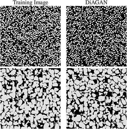
Figure 6. Visual comparison of cuts taken from the TI and DiAGAN generated samples, for the balls dataset (a) and the sand grains dataset (c). Cuts are tiled together for visualization.
The two other 3D examples that are considered here are more difficult because they consider large objects traversing the whole domain. The data sets contain less repetitions and identifying the underlying statistical distribution from these images is therefore more difficult than for the two previous cases. In addition, for the folded layers dataset (Figure 2B) the orientation of the layers varies inside the training image and therefore there is a non-stationarity in the training data. The results from DiAGAN for this example (Figure 7) show less variability in the orientations or in the variograms, but a correct visual reconstruction of the layers. Continuous fold layers that were solid in the TI present holes or imperfections in the generated examples. We therefore observe a reduction of the sill of the variogram and a connectivity that remains high instead of fluctuating for facies 0, while often dropping faster than in the TI for facies 1. The differences between the statistical estimates of the mean and standard deviations are obviously important indicating that the DiAGAN model in this case does not capture all the structure of the examples.
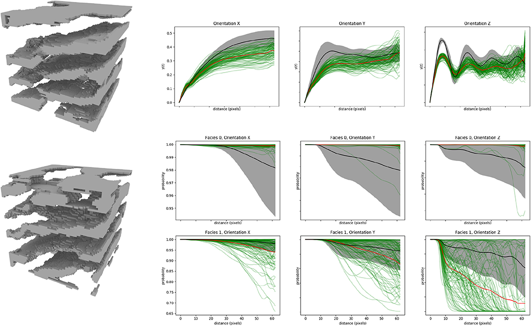
Figure 7. Results of DiAGAN on the categorical fold dataset (b). The three upper curves present the variogram of 100 DiAGAN realizations (green) and their mean (red) along the three axis. The black curve is the mean of observations in the TI for samples of the same size, while the gray area is this mean plus or minus the observed standard deviation. Middle and bottom curves present the connectivity curve of the two facies of the image along the three axes, with the same color conventions.
Finally, for the channelized reservoir case (Figure 2D), DiAGAN simulated the channels from the 2D sections pretty well (Figure 8), although the output is noisier than the reference. The structure and form of the TI is reproduced with satisfactory accuracy as well as the directional variograms and connectivity functions.
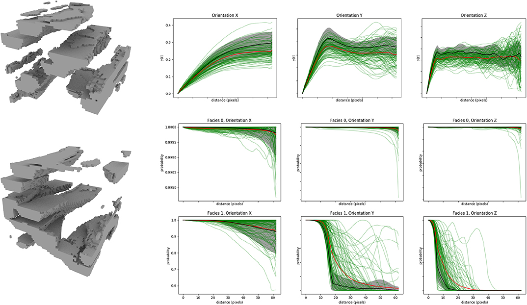
Figure 8. Results of DiAGAN on the procedurally generated channel dataset (d). The three upper curves present the variogram of 100 DiAGAN realizations (green) and their mean (red) along the three axis. The black curve is the mean of observations in the TI for samples of the same size, while the gray area is this mean plus or minus the observed standard deviation. Middle and bottom curves present the connectivity curve of the two facies of the image along the three axes, with the same color conventions.
To conclude that part, these 4 examples show that DiAGAN can generate 3D realizations that are close to the 3D references from 2D examples. There are some differences but one has to remember that the simulation of 3D structures from only 2D cross-sections is a problem that is more difficult than the generation of 3D simulations from 3D examples because only a part of the information is provided to the algorithm. It is therefore not surprising that there is a quality loss. If 3D training data is available, a more traditional 3D to 3D GAN should be used to obtain the best quality.
3.3. Realizations From 2D Datasets
We are now considering some examples corresponding to the real potential application of DiAGAN. Only 2D sections are available and the 3D ground truth is absent. The evaluation of DiAGAN's output in these cases is more challenging. As written above, this situation is more difficult than the case in which a set of 3D examples are provided. The algorithm has to compensate the lack of information about the 3D geometries by assuming (implicitly in the case of GAN) some type of regularities or symmetries. This problem was discussed previously in Comunian et al. (2012) for example. It is therefore expected that 3D simulations based only on 2D examples should be of lower quality than 3D simulations based on 3D examples when the geometries of the geological objects are complex. For a rather simple case presenting a high degree of symmetry (like the balls presented in the previous section), the loss of information is moderate and therefore it is easier to reconstruct the 3D objects.
If we consider first the case based on the 2D Strebellian channels taken as a training image in the (X, Y) and (X, Z) planes (Figure 2E1), DiAGAN correctly simulates a three dimensional network of conduits having a circular section in the (Y, Z) plane. The vertical and horizontal connections between the conduits that are visible in Figure 9 are due to the fact that we use the same training image along the (X, Y) and (X, Z) planes. The sinuosity of the channels in the horizontal plane must also be reproduced in the vertical plane and DiAGAN finds a reasonable solution by creating the network of conduits.
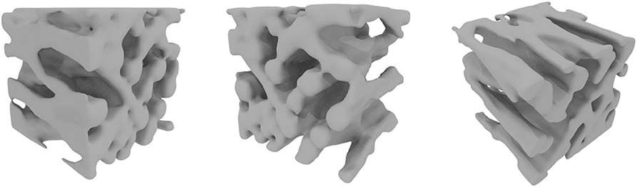
Figure 9. Results of DiAGAN for the 2D channel dataset (Training Images E1 and E2 in Figure 2). Images were obtained by applying a density filter on the original voxel data.
In Figure 10, we present a set of cuts taken from generated samples. The cuts along the (X, Y) and (X, Z) planes resembles the channels from the TI, but they may be broken when a channel moves out of the cut to ensure the 3D continuity that we see in Figure 9. The perpendicular cuts along the (Y, Z) plane are much more isotropic but they depart from the target training image made of disks (Figure 2E2). We think that this discrepancy is due to the fact that the cuts in different directions are not perfectly compatible. Those images have been drawn separately, and despite the effort that we made to respect similar sizes for the object in the common direction, nothing ensures that a 3D geometry with these sections can really exist. DiAGAN is however capable of obtaining a compromise and a reasonable solution in this situation. Finally, we note that the convergence of the FID criteria for this problem is slower and more difficult to reach (see Figure 3) because of the issue described above, i.e., the incompatibility between the cuts along the X and Y axis.
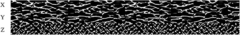
Figure 10. Sample of cuts taken from DiAGAN for the 2D channel dataset (Training Images E1 and E2 in Figure 2).
For the Brussels sands deposit, the situation is easier since the training images have been acquired from an existing 3D structure. In this case, DiAGAN generates some roughly horizontal layers with cross beddings but only oriented along the Y direction as it was indicated in the training data set (Figure 11). The simulations are slightly noisy but the cuts sampled in the 3D simulations (Figure 12) show very well that the cross bedding occurs only in the Y axis plane. The quality of the results is pretty similar to what was obtained earlier with MPS techniques (see Figure 18 in Comunian et al., 2012).
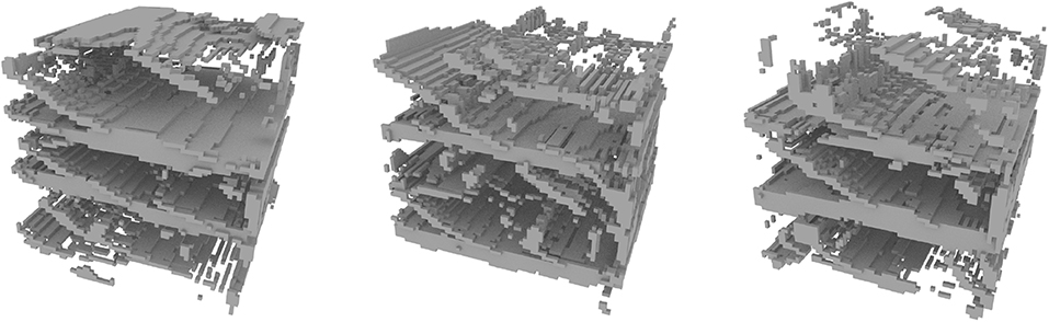
Figure 11. Results of DiAGAN on the Brussel's sand deposit dataset (Training Images F1 and F2 in Figure 2).
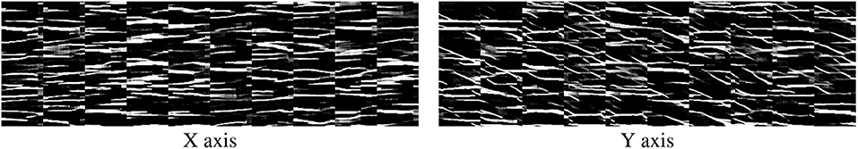
Figure 12. Sample of cuts taken from DiAGAN for Brussel's sand deposit TI (Training Images F1 and F2 in Figure 2).
4. Discussion and Conclusion
Generative adversarial networks represent a new and really different method to generate random fields having a predefined spatial structure (prior distribution). This has already been shown and experimented by several authors (Laloy et al., 2017, 2018; Mosser et al., 2017a).
The main novel idea presented in this paper is to introduce a cut sampler in the GAN process between the generator and the discriminator. Our numerical experiments show that this very simple idea makes it possible to reconstruct 3D parameter fields from a series of 2D examples. This is the main contribution of the paper since this was impossible with the methods cited above. We have tested the idea on a series of simple situations and the results are of comparable quality with those obtained with an MPS method previously published (Comunian et al., 2012). Our experiments demonstrate the feasibility of the approach. It is also to notice that although all experiments generated 64x64x64 images, which is a good trade-off between complexity and memory usage, an algorithm like DiAGAN is able to produce images of any size without retraining, by simply providing a latent noise vector of greater or smaller dimension. This is the main interest of fully convolutional architectures for both the generator and the discriminator (see Table 1). Note that if 3D examples are available, the traditional GANs are expected to generate better simulations because they will account for the complete 3D information. The idea is not to replace existing GAN implementations with DiAGAN. The quality of the simulations obtained for example by Laloy et al. (2018) or Zhang et al. (2019) are excellent. The idea here is to show how these techniques may be slightly modified to generate 3D realizations when only 2D examples are available as it often occurs in practice.
The DiAGAN method could be further improved or extended. One question that was not explored in this work is the effect of using one single random cut per direction or more cuts. The argument to use one cut only per direction was to keep the algorithm as efficient as possible. We have seen in the numerical experiments that the random cut allowed to obtain results of rather good quality. More cuts may improve the quality but would imply more computations and would slow down the method. Further research could investigate if this is worth doing or not.
Another point that could be improved is the fact that the input of the critic is stacked. It forces the cuts to have the same size, and thus to have cubic realizations. In order to have realizations of any shape, it would be pretty straightforward to have different critics for the different orientations. This could also be relevant from a quality point of view, since these parts will be independently trained to identify different patterns. It is therefore possible that this approach would improve the quality of non-symmetrical examples (for example the channels).
On top of this, while DiAGAN demonstrated satisfactory results on various architectures, it is very likely that the algorithm could benefit from recent and future state of the art techniques in Deep Learning, like more efficient neural network architectures. This could improve both the quality of the outputs and the training time.
Finally, at the moment DiAGAN is not conditional. For geoscience applications, this is a requirement. Some methods have already been developed to condition the GANs to hard data (Zhang et al., 2019). In the future similar techniques should also be implemented in DiAGAN to make it applicable for real applications. What is less clear at the moment is how non-stationarities in patterns may be controlled. In traditional MPS, we can force some trends and describe rather precisely how the probabilities of finding different facies may vary in space as a function of some geological knowledge. This has still to be investigated for the GANs.
As compared to the MPS approach, the main advantage of DiAGAN is the possibility to use the latent input space of Gaussian vectors. Indeed, generating a sample using DiAGAN consists in feeding the generator with a latent vector and applying all the layers. This is very efficiently done on modern computers and GPUs. One can expect a speed-up of several order of magnitude compared to more traditional multiple-point statistics. The fact that the latent space is continuous, differentiable, and that it is fast to generate realizations makes this approach potentially very efficient for inverse problem solving. This path has been explored recently for example by Mosser et al. (2019), Laloy et al. (2019) or Liu et al. (2019). However, one remaining issue is that the inverse problem will involve the computation of a forward model using the fields generated with the GANs, and if these fields are discrete (like those studied in this paper), it is possible that the response of the forward model may become discontinuous and not differentiable, posing an issue in the inverse problem formulation. This has still to be explored to better identify the domains of application of these techniques.
Back to the computing time aspects, one has also to remember that training time is still long and can last up to several days of computation. This means that for the moment, if a reasonable number of simulations are needed (several hundreds for example), MPS is still faster. Of course, it depends on the dimension of the problem, the complexity of the patterns to simulate, and the size of the training data set.
As of today, Generative Adversarial Networks represent a very interesting alternative to classical geostatistics clearly worth exploring. Their strength are different from the current state of the art methods, which make them a good complementary method.
Data Availability Statement
The datasets presented in this study can be found in online repositories. The names of the repository/repositories and accession number(s) can be found below: https://github.com/randlab/diaGAN.
Author Contributions
All the coding and numerical experiments were conducted by GC, the idea of DiAGAN emerged from discussions between GC, PR, and SL, and the project was supervised by PR. The writing and editing of the paper was done by GC, PR, and SL.
Funding
PR was partly funded by the SNF project Phenix (200020_182600/1) during that work.
Conflict of Interest
The authors declare that the research was conducted in the absence of any commercial or financial relationships that could be construed as a potential conflict of interest.
Acknowledgments
The authors of the paper would like to thank Przemyslaw Juda for his support and providing the codes for the quality assessment of the realizations, Dr. Boris Galvan and Prof. Stephen A. Miller for having provided access to the GPU cluster of their team, and Prof. Marijke Huysmans for having shared with us the Brussel sands data set. The DiAGAN code and the data sets are accessible online via the github repository: https://github.com/randlab/diaGAN. Note that two implementations are proposed, one using pytorch and one using tensorflow. They provide similar results while they are implemented slightly differently. This illustrates that the method is rather robust.
Footnotes
1. ^http://trainingimages.org/training-images-library.html
2. ^https://www.imperial.ac.uk/earth-science/research/research-groups/perm/research/pore-scale-modelling/micro-ct-images-and-networks/sand-pack-f42a/
References
Adler, P., Jacquin, C. G., and Quiblier, J. (1990). Flow in simulated porous media. Int. J. Multiphase Flow 16, 691–712. doi: 10.1016/0301-9322(90)90025-E
Arjovsky, M., Chintala, S., and Bottou, L. (2017). Wasserstein GAN. arXiv preprint arXiv:1701.07875.
Barfod, A. A., Straubhaar, J., Høyer, A.-S., Hoffimann, J., Christiansen, A. V., Møler, I., et al. (2018). Hydrostratigraphic modelling using multiple-point statistics and airborne transient electromagnetic methods. Hydrol. Earth Syst. Sci. 22, 3351–3373. doi: 10.5194/hess-22-3351-2018
Boucher, A., Gupta, R., Caers, J., and Satija, A. (2010). “Tetris: a training image generator for SGEMs,” Paper Presented at Proceedings of 23nd SCRF Annual Affiliates Meeting (Palo Alto, CA: Stanford University).
Chan, S., and Elsheikh, A. H. (2017). Parametrization and generation of geological models with generative adversarial networks. arXiv preprint arXiv:1708.01810.
Chen, Q., Mariethoz, G., Liu, G., Comunian, A., and Ma, X. (2018). Locality-based 3-d multiple-point statistics reconstruction using 2-d geological cross sections. Hydrol. Earth Syst. Sci. 22, 6547–6566. doi: 10.5194/hess-22-6547-2018
Comunian, A., Renard, P., and Straubhaar, J. (2012). 3D multiple-point statistics simulation using 2D training images. Comput. Geosci. 40, 49–65. doi: 10.1016/j.cageo.2011.07.009
Cordua, K. S., Hansen, T. M., Gulbrandsen, M. L., Barnes, C., and Mosegaard, K. (2016). Mixed-point geostatistical simulation: a combination of two-and multiple-point geostatistics. Geophys. Res. Lett. 43, 9030–9037. doi: 10.1002/2016GL070348
de Marsily, G., Delay, F., Goncalves, J., Renard, P., Teles, V., and Violette, S. (2005). Dealing with spatial heterogeneity. Hydrogeol. J. 13, 161–183. doi: 10.1007/s10040-004-0432-3
Feng, J., Teng, Q., He, X., and Wu, X. (2018). Accelerating multi-point statistics reconstruction method for porous media via deep learning. Acta Mater. 159, 296–308. doi: 10.1016/j.actamat.2018.08.026
Gadelha, M., Maji, S., and Wang, R. (2017). “3D shape induction from 2D views of multiple objects,” in 2017 International Conference on 3D Vision (3DV) (Qingdao: IEEE), 402–411. doi: 10.1109/3DV.2017.00053
Gadelha, M., Rai, A., Maji, S., and Wang, R. (2019). Inferring 3D shapes from image collections using adversarial networks. arXiv preprint arXiv:1906.04910. doi: 10.1007/s11263-020-01335-w
Gerke, K. M., and Karsanina, M. V. (2015). Improving stochastic reconstructions by weighting correlation functions in an objective function. Europhys. Lett. 111:56002. doi: 10.1209/0295-5075/111/56002
Goodfellow, I., Pouget-Abadie, J., Mirza, M., Xu, B., Warde-Farley, D., Ozair, S., et al. (2014). “Generative adversarial nets,” in Advances in Neural Information Processing Systems, eds Z. Ghahramani, M. Welling, C. Cortes, N. D. Lawrence, and K. Q. Weinberger (Montreal, QC: Neural Information Processing Systems Foundation, Inc.), 2672-2680.
Gulrajani, I., Ahmed, F., Arjovsky, M., Dumoulin, V., and Courville, A. C. (2017). “Improved training of Wasserstein GANs,” in Advances in Neural Information Processing Systems, eds I. Guyon, U. V. Luxburg, S. Bengio, H. Wallach, R. Fergus, S. Vishwanathan, and R. Garnett (Long Beach, CA: Neural Information Processing Systems Foundation, Inc), 5769-5779.
Heusel, M., Ramsauer, H., Unterthiner, T., Nessler, B., and Hochreiter, S. (2017). “GANs trained by a two time-scale update rule converge to a local Nash equilibrium,” in Advances in Neural Information Processing Systems, eds I. Guyon, U. V. Luxburg, S. Bengio, H. Wallach, R. Fergus, S. Vishwanathan, and R. Garnett (Long Beach, CA: Neural Information Processing Systems Foundation, Inc), 6626–6637.
Hu, L., and Chugunova, T. (2008). Multiple-point geostatistics for modeling subsurface heterogeneity: a comprehensive review. Water Resour. Res. 44. doi: 10.1029/2008WR006993
Huysmans, M., and Dassargues, A. (2011). Direct multiple-point geostatistical simulation of edge properties for modeling thin irregularly shaped surfaces. Math. Geosci. 43:521. doi: 10.1007/s11004-011-9336-7
Ioffe, S., and Szegedy, C. (2015). Batch normalization: accelerating deep network training by reducing internal covariate shift. arXiv preprint arXiv:1502.03167.
Journel, A., and Zhang, T. (2006). The necessity of a multiple-point prior model. Math. Geol. 38, 591–610. doi: 10.1007/s11004-006-9031-2
Karsanina, M. V., and Gerke, K. M. (2018). Hierarchical optimization: fast and robust multiscale stochastic reconstructions with rescaled correlation functions. Phys. Rev. Lett. 121:265501. doi: 10.1103/PhysRevLett.121.265501
Kessler, T. C., Comunian, A., Oriani, F., Renard, P., Nilsson, B., Klint, K. E., et al. (2013). Modeling fine-scale geological heterogeneity-examples of sand lenses in tills. Groundwater 51, 692–705. doi: 10.1111/j.1745-6584.2012.01015.x
Kingma, D. P., and Ba, J. (2014). ADAM: a method for stochastic optimization. arXiv preprint arXiv:1412.6980.
Laloy, E., Hérault, R., Jacques, D., and Linde, N. (2018). Training-image based geostatistical inversion using a spatial generative adversarial neural network. Water Resour. Res. 54, 381–406. doi: 10.1002/2017WR022148
Laloy, E., Hérault, R., Lee, J., Jacques, D., and Linde, N. (2017). Inversion using a new low-dimensional representation of complex binary geological media based on a deep neural network. Adv. Water Resour. 110, 387–405. doi: 10.1016/j.advwatres.2017.09.029
Laloy, E., Linde, N., Ruffino, C., Hérault, R., Gasso, G., and Jacques, D. (2019). Gradient-based deterministic inversion of geophysical data with generative adversarial networks: is it feasible? Comput. Geosci. 110:104333. doi: 10.1016/j.cageo.2019.104333
Lemmens, L., Rogiers, B., Jacques, D., Huysmans, M., Swennen, R., Urai, J. L., et al. (2019). Nested multiresolution hierarchical simulated annealing algorithm for porous media reconstruction. Phys. Rev. E 100:053316. doi: 10.1103/PhysRevE.100.053316
Linde, N., Renard, P., Mukerji, T., and Caers, J. (2015). Geological realism in hydrogeological and geophysical inverse modeling: a review. Adv. Water Resour.86, 86–101. doi: 10.1016/j.advwatres.2015.09.019
Liu, Y., Sun, W., and Durlofsky, L. J. (2019). A deep-learning-based geological parameterization for history matching complex models. Math. Geosci. 51, 725–766. doi: 10.1007/s11004-019-09794-9
Mariethoz, G., and Caers, J. (2014). Multiple-Point Geostatistics: Stochastic Modeling With Training Images. Chichester: John Wiley & Sons. doi: 10.1002/9781118662953
Mariethoz, G., and Kelly, B. F. (2011). Modeling complex geological structures with elementary training images and transform-invariant distances. Water Resour. Res. 47. doi: 10.1029/2011WR010412
Mariethoz, G., Renard, P., and Straubhaar, J. (2010). The direct sampling method to perform multiple-point geostatistical simulations. Water Resour. Res. 46. doi: 10.1029/2008WR007621
Meerschman, E., Van Meirvenne, M., Mariethoz, G., Islam, M. M., De Smedt, P., Van De Vijver, E., et al. (2014). Using bivariate multiple-point statistics and proximal soil sensor data to map fossil ice-wedge polygons. Geoderma 213, 571–577. doi: 10.1016/j.geoderma.2013.01.016
Mosser, L., Dubrule, O., and Blunt, M. J. (2017a). Reconstruction of three-dimensional porous media using generative adversarial neural networks. Phys. Rev. E 96:043309. doi: 10.1103/PhysRevE.96.043309
Mosser, L., Dubrule, O., and Blunt, M. J. (2017b). Stochastic reconstruction of an oolitic limestone by generative adversarial networks. Trans. Porous Media 125, 1–23. doi: 10.1007/s11242-018-1039-9
Mosser, L., Dubrule, O., and Blunt, M. J. (2019). Deepflow: history matching in the space of deep generative models. CoRR abs/1905.05749.
Okabe, H., and Blunt, M. J. (2007). Pore space reconstruction of vuggy carbonates using microtomography and multiple-point statistics. Water Resour. Res. 43. doi: 10.1029/2006WR005680
Oriani, F., Straubhaar, J., Renard, P., and Mariethoz, G. (2014). Simulation of rainfall time series from different climatic regions using the direct sampling technique. Hydrol. Earth Syst. Sci. 18, 3015–3031. doi: 10.5194/hess-18-3015-2014
Radford, A., Metz, L., and Chintala, S. (2015). Unsupervised representation learning with deep convolutional generative adversarial networks. arXiv preprint arXiv:1511.06434.
Salimans, T., Goodfellow, I., Zaremba, W., Cheung, V., Radford, A., and Chen, X. (2016). “Improved techniques for training GANs,” in Advances in Neural Information Processing Systems, eds D. D. Lee, M. Sugiyama, U. V. Luxburg, I. Guyon, and R. Garnett (Barcelona: Neural Information Processing Systems Foundation, Inc), 2234-2242.
Strebelle, S. (2002). Conditional simulation of complex geological structures using multiple-point statistics. Math. Geol. 34, 1–21. doi: 10.1023/A:1014009426274
Ulyanov, D., Vedaldi, A., and Lempitsky, V. (2016). Instance normalization: the missing ingredient for fast stylization. arXiv preprint arXiv:1607.08022.
Vannametee, E., Babel, L., Hendriks, M., Schuur, J., De Jong, S., Bierkens, M., et al. (2014). Semi-automated mapping of landforms using multiple point geostatistics. Geomorphology 221, 298–319. doi: 10.1016/j.geomorph.2014.05.032
Wei, L.-Y., Lefebvre, S., Kwatra, V., and Turk, G. (2009). “State of the art in example-based texture synthesis,” in Eurographics 2009, State of the Art Report, EG-STAR (Munich: Eurographics Association), 93–117.
Yeong, C., and Torquato, S. (1998). Reconstructing random media. Phys. Rev. E 57:495. doi: 10.1103/PhysRevE.57.495
Zhang, T.-F., Tilke, P., Dupont, E., Zhu, L.-C., Liang, L., and Bailey, W. (2019). Generating geologically realistic 3D reservoir facies models using deep learning of sedimentary architecture with generative adversarial networks. Petrol. Sci. 16, 541–549. doi: 10.1007/s12182-019-0328-4
Keywords: geology, heterogeneity, stochastic model, groundwater, generative adversarial network, deep learning
Citation: Coiffier G, Renard P and Lefebvre S (2020) 3D Geological Image Synthesis From 2D Examples Using Generative Adversarial Networks. Front. Water 2:560598. doi: 10.3389/frwa.2020.560598
Received: 09 May 2020; Accepted: 17 August 2020;
Published: 28 October 2020.
Edited by:
Eric Laloy, Belgian Nuclear Research Centre, BelgiumReviewed by:
Kirill M. Gerke, Russian Academy of Sciences (RAS), RussiaZhaoyang Larry Jin, Stanford University, United States
Ahmed H. Elsheikh, Heriot-Watt University, United Kingdom
Copyright © 2020 Coiffier, Renard and Lefebvre. This is an open-access article distributed under the terms of the Creative Commons Attribution License (CC BY). The use, distribution or reproduction in other forums is permitted, provided the original author(s) and the copyright owner(s) are credited and that the original publication in this journal is cited, in accordance with accepted academic practice. No use, distribution or reproduction is permitted which does not comply with these terms.
*Correspondence: Guillaume Coiffier, Z3VpbGxhdW1lLmNvaWZmaWVyQGlucmlhLmZy