Automated Cloud Based Long Short-Term Memory Neural Network Based SWE Prediction

Snow derived water is a critical component of the US water supply. Measurements of the Snow Water Equivalent (SWE) and associated predictions of peak SWE and snowmelt onset are essential inputs for water management efforts. This paper aims to develop an integrated framework for real-time data ingestion, estimation, prediction and visualization of SWE based on daily snow datasets. In particular, we develop a data-driven approach for estimating and predicting SWE dynamics using the Long Short-Term Memory neural network (LSTM) method. Our approach uses historical datasets (precipitation, air temperature, SWE, and snow thickness) collected at NRCS Snow Telemetry (SNOTEL) stations to train the LSTM network and current year data to predict SWE behavior. The performance of our prediction was compared for different prediction dates and prediction training datasets. Our results suggest that the proposed LSTM network can be an efficient tool for forecasting the SWE timeseries, as well as Peak SWE and snowmelt timing. Results showed that the window size impacts the model performance (where the Nash Sutcliffe efficiency (NSE) ranged from 0.96 to 0.85 and the Rooted Mean Square Error (RMSE) ranged from 0.038 to 0.07) with an optimum number that should be calibrated for different stations and climate conditions. In addition, by implementing the LSTM prediction capability in a cloud based site-monitoring platform, we automate model-data integration. By making the data accessible through a graphical web interface and an underlying API which exposes both training and prediction capabilities. The associated results can be made easily accessible to a broad range of stakeholders.

Introduction

Accurate estimation and prediction of snow water equivalent (SWE) in mountain watersheds has been a longstanding challenge (Bair et al., 2018), while, it is a key metric used by hydrologists and water managers to assess water resources in snow-dominated catchments or basins (Bales et al., 2006; Painter et al., 2016). SWE is defined as the equivalent amount of water if the snow mass is completely melted. SWE is one of the main parameters used in accurate prediction of snowmelt runoff and snowpack and water supply forecasting (Schneider and Molotch, 2016). Consequently there is substantial interest in forecasting seasonal SWE dynamics, including parameters such as peak SWE and snowmelt timing onset (Odei et al., 2009). This snowmelt timing is critical for ecological processes in snow-dominated regions, controlling plant dynamics, net ecosystem exchanges, and soil carbon (Harte et al., 2015; Sloat et al., 2015; Wainwright et al., 2020). Snowmelt timing also drives peak flow timing during which significant nutrient export occurs from the catchments (Carroll et al., 2018). In recognition of its value for water resource prediction SWE and associated measurements (temperature, precipitation, windspeed and direction, and snow thickness) are measured across the west area by the U.S. Natural Resource Conservation Service's (NRCS) through over 800 automated data collection stations known as SNOTEL (SNOw TELemetry) stations, as well as by airborne observations (Painter et al., 2016). Stations are typically located in small clearings in evergreen forests. Data from these stations is transferred multiple times a day to a central database, from where the data is publicly accessible through web interfaces and software APIs. Each SNOTEL station has a long record of historical data, often more than 30 years, encompassing a variety of metrological conditions at each site. This results in typically more than 10,000 data points. In addition, snow accumulation and melting is a highly heterogeneous process affected by a complex terrain or regional scale atmospheric forcing which support us to use deep learning method for SWE forecasting.

There is a long standing interest in the use of probabilistic forecasting and Artificial Neural Networks (ANN) such as recurrent neural networks (RNNs) (Kumar et al., 2004) for hydrology and SWE forecasting (Huang and Cressie, 1996; Winstral et al., 2019; Magnusson et al., 2020). More recently deep learning methods such as the long short-term memory network (LSTM) have demonstrated a significant promise in hydrological time series analysis and forecasting (Xiang et al., 2020), such as soil moisture modeling (Fang et al., 2017), monthly water-table depth predictions (Zhang et al., 2018), and daily or hourly rainfall-runoff modeling (Hu et al., 2018; Kratzert et al., 2018; Le et al., 2019; Fan et al., 2020).

In this paper, we develop the integrated framework of real-time ingestion, estimation/prediction and visualization (webinterface) of the snow dynamics based on SNOTEL generated time-series data. In particular, we demonstrate the feasibility of using LSTM trained on for predicting future SWE dynamics. Although we use a few selected SNOTEL stations, our framework is general, and hence, it can be used for other stations across the US. In addition, the feasibility of automating and exposing this capability through a webinterface and an underlying API is demonstrated. It includes quality control, flagging and interpolation, which is often a bottleneck of applying deep learning to environmental datasets. We believe that this framework makes the predictions and deep learning easily accessible to different interested parties for public use or stakeholder use.

Materials and Methods

Study Area

In this paper, we focus on five SNOTEL stations, which are located in Western Colorado within the central Rocky Mountains (Figure 1). Our interest in this area is associated with work done by several of the authors on the multiyear, multi-institution Department of Energy funded research effort (the Lawrence Berkeley National Lab (LBNL) Watershed Science Focus Area (SFA) (Hubbard et al., 2018), which focuses on the East River Watershed located near Crested Butte, Colorado. The East River watershed measures ~300 km². It includes montane to alpine ecosystems with an elevation ranging from 2,500 m to 4,000 m. The vegetation in this watershed is diverse, including mixed conifer forest, aspen forest, and open meadows (Harte et al., 2015). Streamflow is dominated by snowmelt in spring and summer (Markstrom et al., 2012). This watershed is a typical headwater catchment in the Colorado River Basin. As the Colorado River Basin provides 75% of the water demand for 40 million people in seven states and two countries (Deems et al., 2013) an understanding of hydro-biogeochemical processes in these headwaters catchments is of obvious value and interest.

FIGURE 1

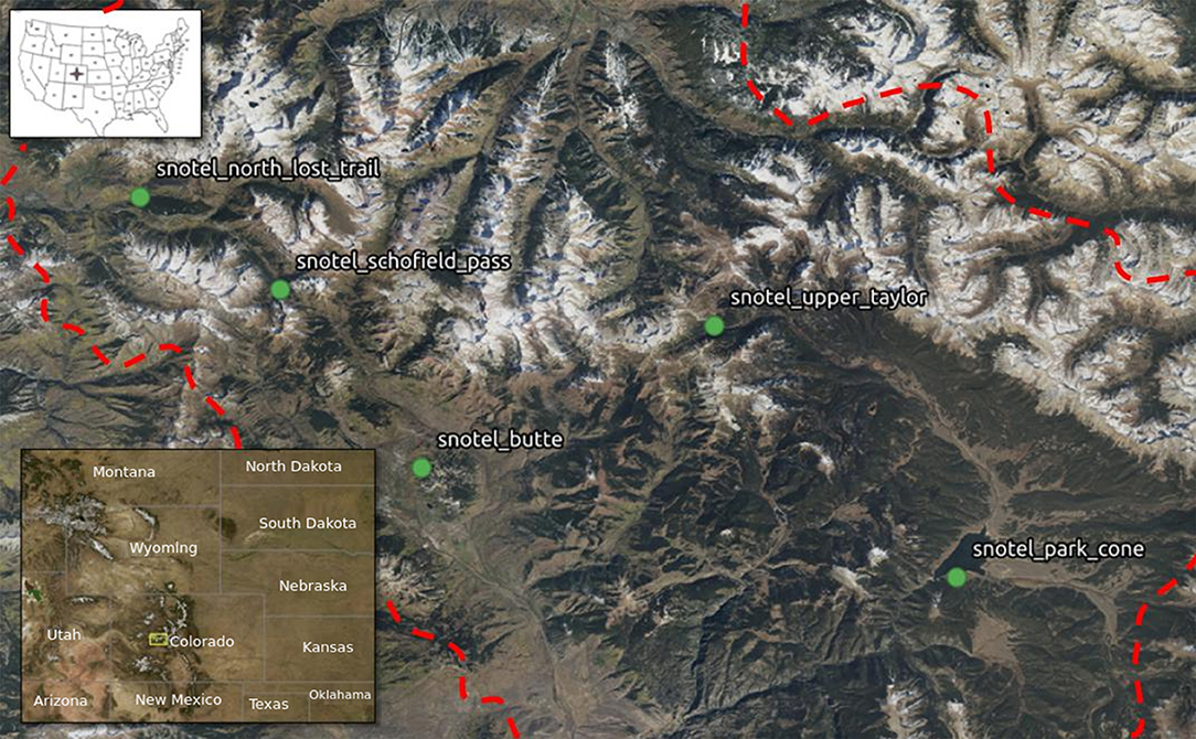
Figure 1. Location and names of the five SNOTEL Stations used in this study (red dash line: East River watershed boundary).

Data

Data types collected at SWE stations varies across stations. As far as we can ascertain, all stations collect SWE, snow thickness, precipitation and air temperature. Many stations also collect other environmental parameters such as wind speed and wind direction, air pressure and incoming broadband solar radiation. While in general data quality and continuity is high, there are instances (especially in the data from the early 2000s where SNOTEL data is not continuous, is noisy or has outliers. In this paper we have not included gapfilling or noise elimination strategies as we limited our prediction to use data from five selected stations for the last 10 years which are of good quality (Figure 2). However, robust error handling strategies need to be built in for real life applications.

FIGURE 2

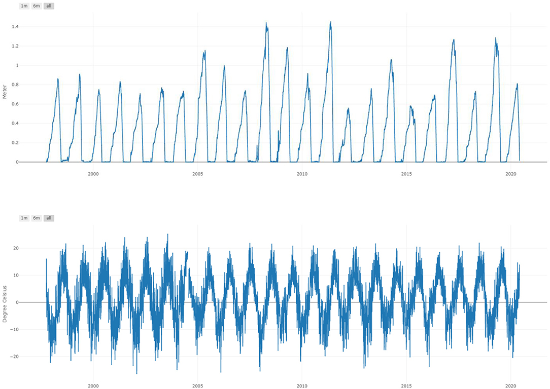
Figure 2. Example of data used in this study. Top: SWE data from the Schofield station. Bottom: Temperature at the Schofield station.

Methods

Project Data Ingestion and Exposure Through Cloud Based API

We have developed robust capabilities to automatically retrieve, normalize (variable names, units, and timestamps), ingest and link heterogeneous data (hydrological, geochemical, geophysical, microbiological, and remote sensing) from numerous public and project specific data sources. These data are stored in project specific relational databases. The datamodel underlying these databases is a substantially modified version of the ODM2 (Observation Data Model version 2) datamodel (Horsburgh et al., 2016).

Data in the database is accessible to both through a web interface (which allows both data visualization in a variety of manners and data download) and a rich API. While the public data hosted in our database can be obtained by users themselves through APIs provided by different organizations, our architecture allows users both to access and locate uniform data across the project site using a single API call as well as provides advanced visualization and analytical capabilities.

An example of the capabilities of this interface is shown in Figure 3, which shows the SWE for the Butte SNOTEL Station for different water years (defined by the USGS as the period between October 1st of 1 year and September 30th of the next). Thus, the water year 2020 runs from 10-1-2019 until 9-30-2020.

FIGURE 3

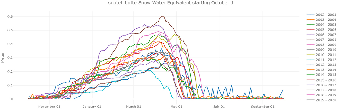
Figure 3. Graph of year over year SWE measured at the Butte SNOTEL station generated by the web interface of our cloud based data management system.

Long Short-Term Memory Network

The prediction of time series behavior is of interest for a wide range of applications. Numerous statistical and machine learning approaches exist to predict time series behavior (Fawaz et al., 2019). When dealing with long-term dependencies, traditional feed forward Artificial neural networks (ANNs) are limited (Bengio et al., 1994; Fang et al., 2017). However, the Long Short-Term Memory (LSTM) network method is well-suited for long term dependencies (Hochreiter and Schmidhuber, 1997; Fan et al., 2020). LSTM is a deep neural network (DNN) method which has been successfully applied in various fields (Sahoo et al., 2019) for especially for time sequence prediction problems.

LSTM is well-suited to classify, process, and predict time series given time lags of unknown duration. It can be trained on and deal with long sequences and does not rely on a pre-specified window lagged observation as input (Kratzert et al., 2018). In addition, LSTM is well-suited to deal with time series prediction problems with multiple input variables (Le et al., 2019).

In order to use LSTM, we first need to train and calibrate a model. Once this is done the model can be used to predict future values. Figure 4 shows a schematic of the one-step iteration in the LSTM training/calibration procedure (Fan et al., 2020).

FIGURE 4

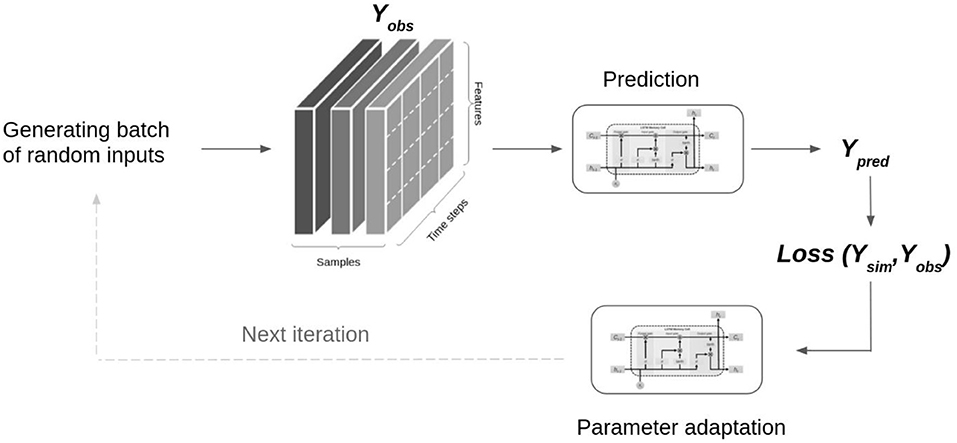
Figure 4. One step iteration of the training process in the LSTM approach.

A random batch of input data, consisting of several independent training samples (depicted by the gray colors) that is used in each step. Thus, the input to every LSTM prediction layer is three dimensional, with the three dimensions being samples (or sequences), time steps and features (observations at a timestep). As can be seen in Figure 4 each training sample consists of several days (timesteps) of look-back data and one target value (Y) to predict. Therefore, the number of samples refer to the number of observations fed into the LSTM network. The number of timesteps or lookback, describes the time window (past data) needed by the LSTM. In each LSTM training iteration step, some of the available training data is used to update some model parameters such as the weights, biases, and learnable network parameters. This update is done in such a way that the loss function is reduced. The loss function is computed from the observed training samples and the network's predictions. In this study, we used the mean-square-error as the loss function for parameter optimization (Kratzert et al., 2018). The gradient descent optimization algorithm is used to reduce the loss function which is equivalent to the unexplained fraction of variance (Xiang et al., 2020).

In building a LSTM, after normalizing the raw data, the dataset is first made suitable for a supervised learning problem by splitting into test and training data and by formatting the data in the right input format. Following common practices 60% of data is used for training and 40% is used for validation. After the model is trained and validated, the model can then be used to generates predictions for the future values. The model performance can be evaluated by using testing datasets. Forecasting uncertainties can be represented with confidence intervals. These confidence intervals give us an interval within which we expect the real value to lie with a specified probability that uses standard deviation and mean values of previous observations and current real data. The range of confidence intervals communicates our confidence in the uncertainty associated with the forecast. The confidence intervals are calculated by standard deviation, percentage multiplier and forecast distribution. The percentage multiplier depends on the coverage probability as shown in Table 1 (Hyndman et al., 2018).

TABLE 1

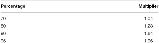
Table 1. Multipliers to be used for confidence intervals.

Application of LSTM to SWE Time-Series Analysis and Prediction

In our prediction problem (and in the software implementation), we assume that we have the SWE time-series up to a specific (generally the current) date in a specific (generally the current) water year, and aim to predict the future SWE from this date for the remainder of the water year based on the historical datasets. As our architecture pulls in new SWE data on a daily basis this prediction is quasi real-time, and in general most interest will be in using our prediction in this mode. However, by allowing the flexibility of providing dates in the past our code allows for performance assessment.

For SWE timeseries forecasting we use the method described above, which is implemented as a python code which uses the Tensorflow (Abadi et al., 2016) and Keras (Chollet et al., 2015) libraries. This code is exposed through an API. The API can be accessed directly programmatically or through a web interface which provides a visual interface to the API (Figure 5). Parameters passed to the API include which SNOTEL location to forecast for, how many years of historic data to use for training, what type of snow years (below average, average, or above average) prediction data to use, and for which date we should predict for.

FIGURE 5

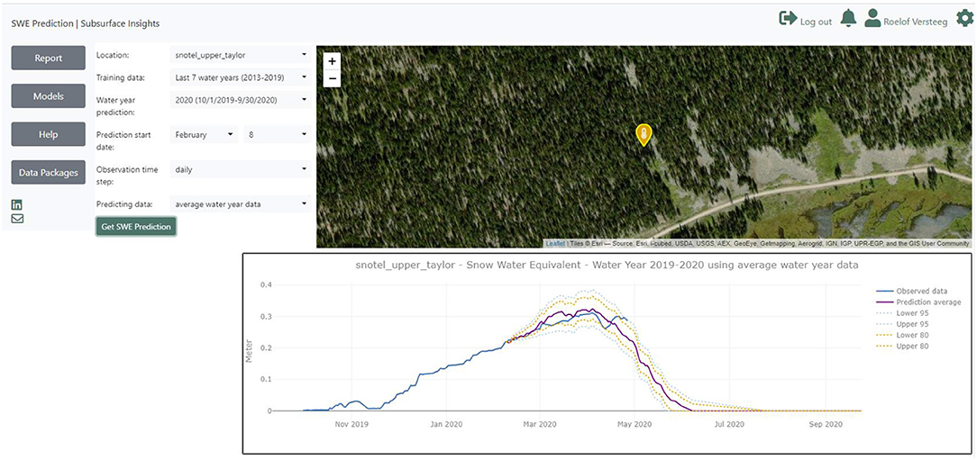
Figure 5. Web interface to the prediction API.

Once our code receives the parameters it first retrieves the raw datasets (which includes SWE, precipitation, snow thickness, and air temperature) needed for prediction through a call to the data API. These are long sequences of thousands of observations for data in previous water years. These sequences are split into samples which are reshaped for the LSTM model. The size of these samples is called the window size (Fan et al., 2020) and has impact on the forecast accuracy.

The reshaped data is used to train the LSTM network. The supervised learning problem is framed as predicting the SWE at a specific day given SWE and associated data (precipitation, snow thickness, and air temperature) up to that day. In our analysis we used training datasets with between 5 and 10 years of recent SNOTEL data, but our code is able to deal with different lengths of data to train the LSTM network.

Once the network is trained, we can use it to make predictions about SWE for a specific water year and date within this year. For this prediction, the model needs the history of SWE over the past months and days in the current water year until the prediction start date. The model then predicts SWE for the remainder of that water year. For the prediction data we allow users to select any of snow years worth of data (e.g. “below average,” “average,” “above average” years) to accommodate different kinds of snow years.

It should be noted that in this study, the proposed LSTM method was tested for several SNOTEL stations in the one watershed (East River watershed), but as automated, it can be used for any other stations in other watershed, hence, the model and the system are not dependent on any dataset and station. As presented in Figure 5, any location (station related to any watershed) can be selected for SWE prediction.

Model Evaluation Criteria

To evaluate forecasting performance, we can use different statistical criteria. The ones we use include the Nash Sutcliffe model efficiency coefficient (NSE) (Nash and Sutcliffe, 1970) and Rooted Mean Square Error (RMSE) which are a widely used performance evaluation method for hydrological modeling (Krause et al., 2005; Arnold et al., 2012). Both of these compare predicted values with observed values. The NSE evaluates the model performance to predict testing data different from the mean and gives the proportion of the initial variance accounted for by the model (Nash and Sutcliffe, 1970). The RMSE is used to evaluate how closely the predicted values match the observed values, based on the relative range of the data.

$\begin{array}{ll}NSE=1-\frac{{\sum }_{i=1}^n{\left(Y_i^o-Y_i^p\right)}^2}{{\sum }_{i=1}^n{\left(Y_i^o-Y^{\prime }\right)}^2}& (1)\end{array}$

$\begin{array}{ll}RMSE=\sqrt{\frac{{\sum }_{i=1}^n{\left(Y_i^o-Y_i^p\right)}^2}{n}}& (2)\end{array}$

where $Y_i^o$, $Y_i^p$ and Y′epresent the observed, predicted and the average observed data at time i respectively. NSE ranges from –∞ to 1, and the value close to 1 is equivalent the better model performance (Arnold et al., 2012). In general, a lower RMSE represents a higher accuracy and a better fit.

Results

Forecasts and Performance

The method described above generates a site-specific LSTM model which can be used to predict SWE. This model can be trained using different datasets (e.g., the last 10 years of data), and be used to predict SWE dynamics in different types of years (low snow, medium snow, high snow years). The model can use any specified start date in the past to evaluate the performance of the approach in SWE forecasting.

We evaluated SWE forecast performance, obtained from LSTM model, by considering 3 month forecasting for different SNOTEL stations (Schofield Pass, Upper Taylor, and Park Cone). The observation data obtained from stations were available until May 1, 2020 and 3 month before this time is February 1, 2020 that was the starting date to forecast. Given these conditions, the performance of the model can be evaluated with the observed data from the stations and the predicted SWE data from the LSTM model. However, the model can use any dates in the past to forecast, hence, it can be invoked programmatically makes it easy to evaluate performance and to use it for scenario modeling. An example of this prediction is shown in Figures 5, 6.

FIGURE 6

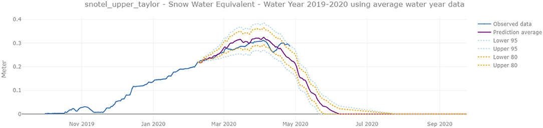
Figure 6. Detail of Figure 5 showing prediction for a start date of February 7. The prediction was made in Note that our prediction matches actual data (available through the end of April) quite well.

Figure 7 shows the SWE prediction for the selected stations. In addition, the uncertainty in the prediction and the match between predicted and observed data for each station are presented in the associated graph for each station. The predicted data is obtained from the LSTM model and current water year data. All the graphs illustrate the both peak SWE and snowmelt timing captured within the confidence interval and therefore the performance is consistent among these three locations. The model and the results are validated by applying criteria such as NSE value, RMSE value. The LSTM model has a narrower range of RMSE between 0.026 m and 0.03 m relative to the Upper Taylor and Schofield Pass station. The value of NSE is also improved from 0.85 (Park Cone) to 0.96 (Schofield Pass). The results illustrate equally good performance. However, since the LSTM model is highly dependent on the meteorological variables such as rainfall, the model with smoother observed data is able to capture more precisely the peak of snowmelt timing and SWE forecast as well. As mentioned, all three stations shown in Figure 7 have acceptable results, although the model performance at Park Cone Station is not as good as the other two stations, this is due to meteorological data (rainfall) which is smoother at the other two stations.

FIGURE 7

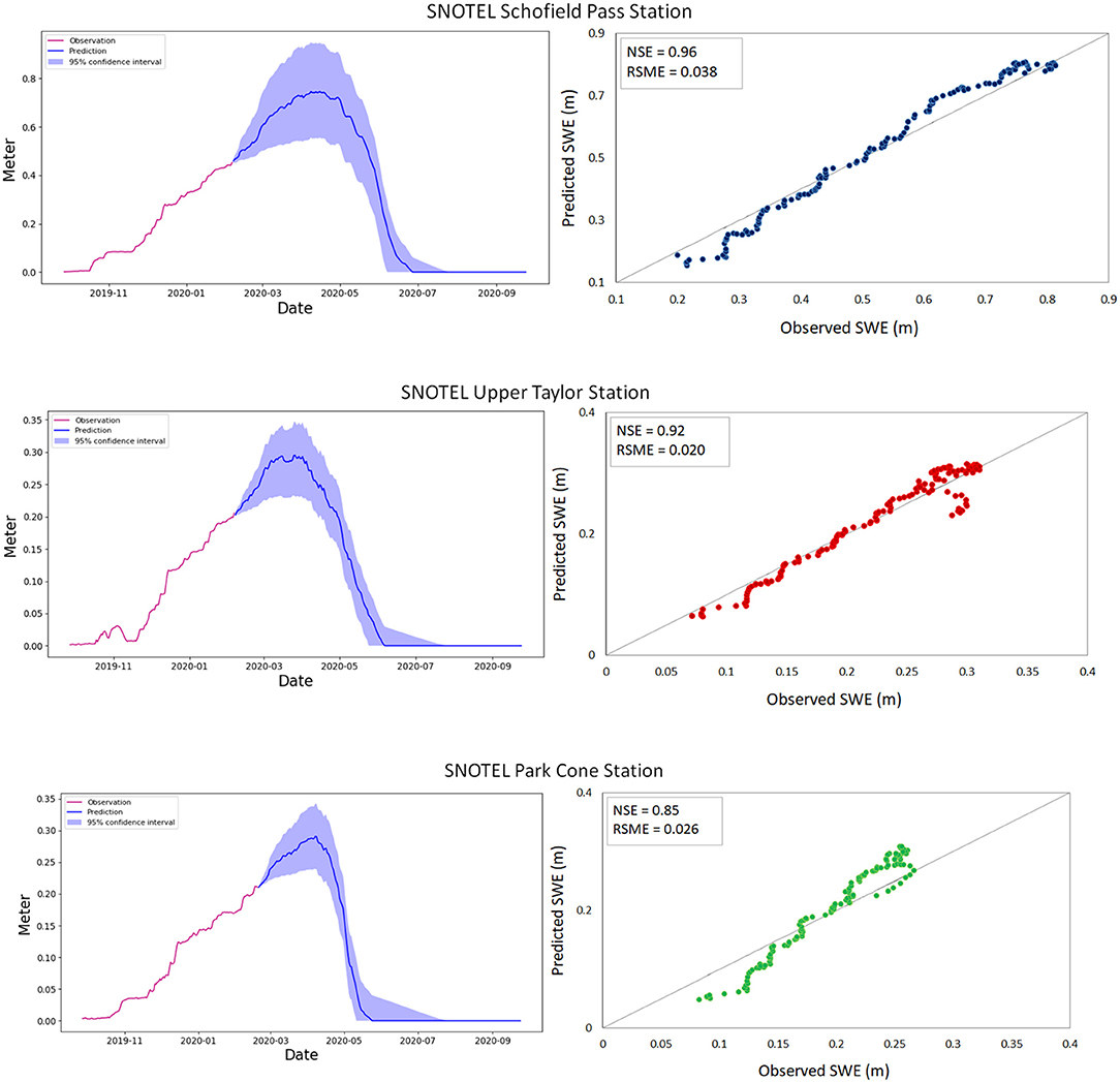
Figure 7. SWE observed and predicted for the current year (2020) with their performance, for SNOTEL Schofield Pass station, SNOTEL Upper Taylor station, and SNOTEL Park Cone station.

We can also evaluate the prediction behavior for different days by changing the starting date. An example of this is shown in Figure 8 which shows the SWE prediction for the SNOTEL Schofield Pass station for different days in the past (from December 1, 2019, to March 1, 2020). This demonstrates the model's ability to predict SWE at any time of the water year. As is expected the confidence interval becomes narrower reduces over time as we get closer to the end of the year (Table 2). In all the cases, the SWE time series are contained within the interval, which validates our methodology.

FIGURE 8

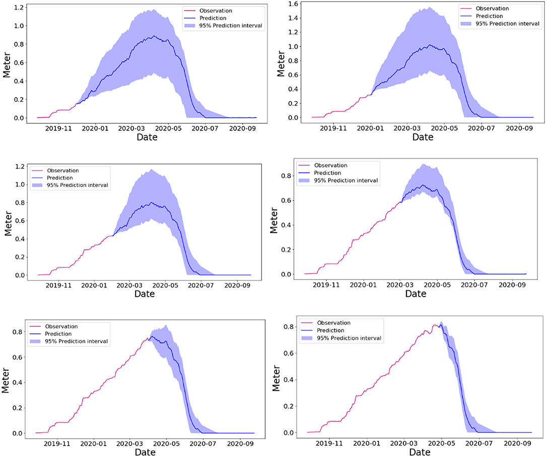
Figure 8. Forecasting from the different past month for the water year 2020.

TABLE 2

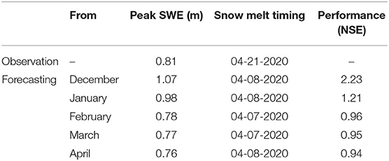
Table 2. Prediction performance for key metrics (peak SWE and Snow melt timing) for different start dates.

Model Parameter Effect

There are multiple model parameters which we can vary in the LSTM network. These include the epoch and the number of historic years we use as training data. In NN applications, the epoch is one cycle through the full training set in which model parameters are updated.

Figure 9 illustrates the LSTM learning process for different numbers of training epochs. It shows how the training network improves from the initial state from scratch (where it has random weights) as we go to 200 epochs.

FIGURE 9

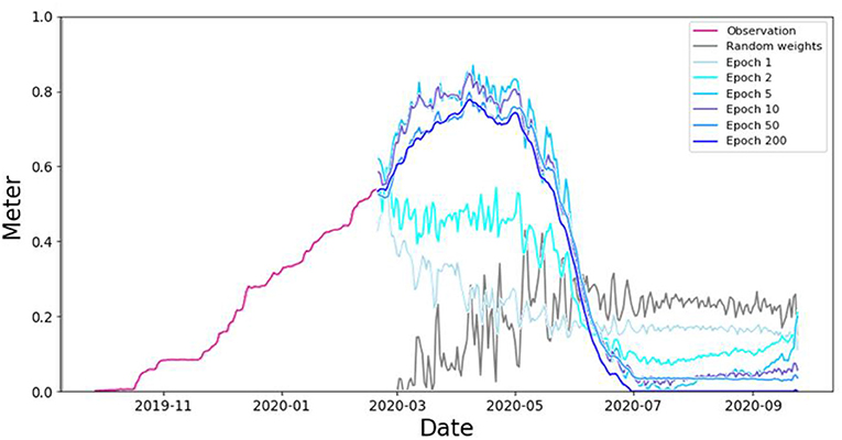
Figure 9. Improvement of SWE prediction during the learning process of the LSTM as the number of epochs increases.

Effect of the Number of Years Used to Train Our Dataset

As mentioned before (and as should be intuitively clear), the number of years of data we use to train our dataset has an impact on the model performance, and it is important to evaluate and analyze this impact. We can evaluate the effect of the number of years used on the model performance (which is represented by Loss function or NSE). We compared 4 different lengths: 2, 5, 10, and 15 years. The comparison results are shown in Figure 10.

FIGURE 10

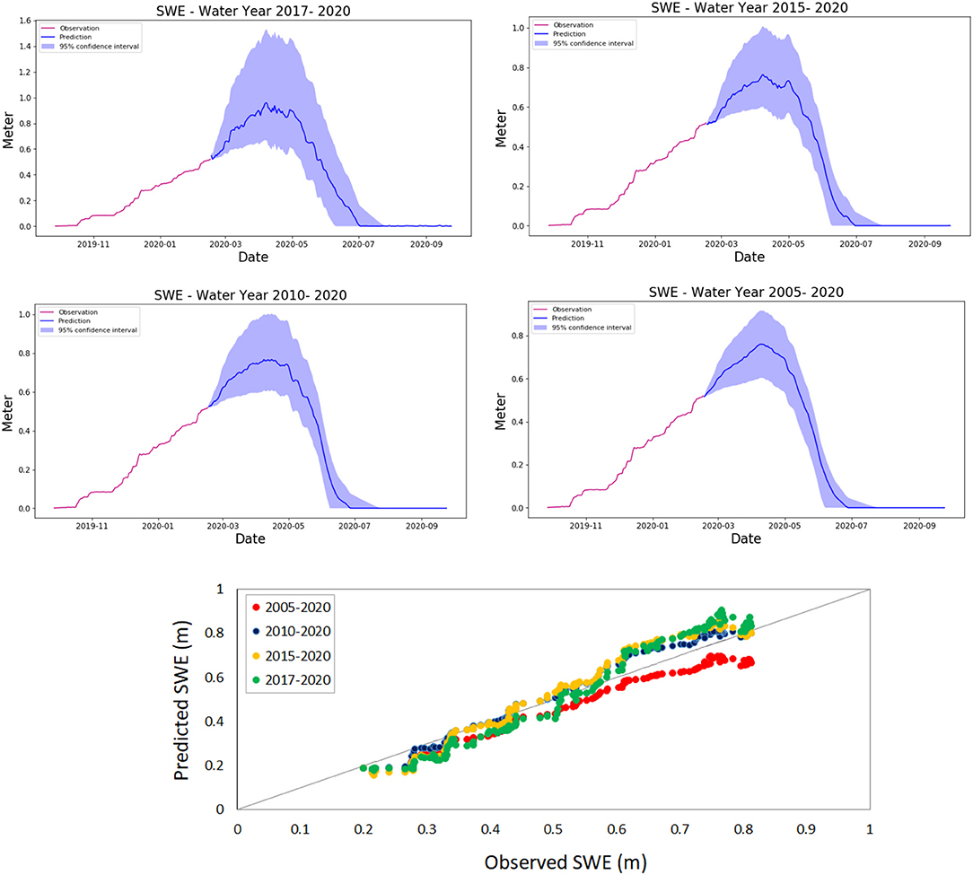
Figure 10. SWE predicted for the different length of years of training data (2, 5, 10, and 15 years).

The statistical results for the overall performances of LSTM models for both length of training data are listed in Table 3. As shown in Table 3, the prediction performed well for the 10 years length (2010–2020), with average NSEs of 0.96 and RSME 0.038. Although we initially expected that increasing the number of years used to train our model (15 years for our model 2005–2020) would have better performance, the 10 years window size performed better. This behavior can be observed in Figure 10, in the Predicted-Observed graph. The blue dots that represent 10 year window size (2010–2020) show a better performance than the red dots that represent the 15 year window size. This may be associated with a shift in system behavior—which would be better expressed in recent data than in older data. In addition, it should be noticed that the confidence interval becomes narrower when the window size increases (Figure 10).

TABLE 3

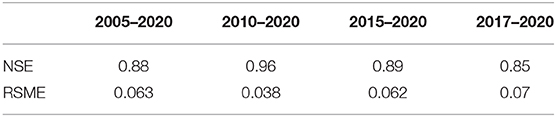
Table 3. Statistics of LSTM model for SWE prediction on the SNOTEL Schofield Pass Station for different window size.

We can combine the results shown in Figures 9–11 which shows the loss function behavior for different lengths of training data. As shown in Figure 11, the Loss function of the LSTM model decreased (or NSE increased) when the length of training data increases. It should be noticed also that when training with longer dataset the curve of the loss function becomes smoother. However, as shown in Table 3 and Figure 10 adding more years of data beyond 10 years does not increase performance. It is interesting to consider why this is, and while a detailed analysis of this falls outside the scope of this paper it could be because SWE characteristics have changed over the last 10 years. If this is the case, more recent SWE behavior would be a better predictor of current behavior than SWE behavior of 15 or 20 years back.

FIGURE 11

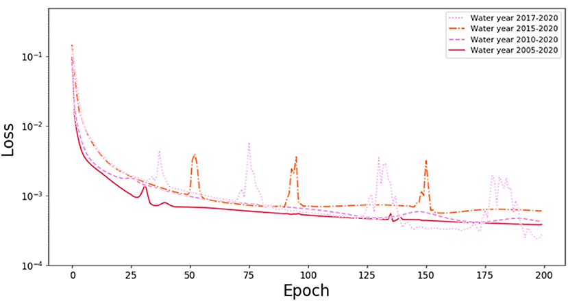
Figure 11. Loss function after 200 epochs for predictions using different water years (2, 5, 10, and 15 years).

LSTM Automation

In this study, we have presented a step-by-step workflow on the SWE prediction by obtaining the metrological data form stations, training the model with the different windows size, checking the confidence interval, plotting the results and calculating the performance of the prediction. However, all these process and capability can be automated at different levels. First by automatically creating trained networks for any SNOTEL site, using API-able approach and creating daily updated predictions using new data for every day by rerunning the prediction. Finally, the predicted results can be delivered to interested end users. This delivery can be either done through an API or through a web interface as shown in Figures 5, 6. Due to the flexibility of the API, the effect of using different training datasets can be rapidly compared.

Discussion

In this study, we demonstrated that LSTM networks can be trained to accurately predict SWE behavior for different NRCS SNOTEL stations. Prediction accuracy and performance were analyzed for different epoch number and length of training data. Our results demonstrate that training data length affects the model performance. While 7–10 years of training data length seems to be suitable for the sites we examined this number should be determined for different stations and climate conditions.

There are multiple other efforts which have focused on SWE. This includes the work by Guan et al. (2013) which retrospectively estimates SWE distribution by using the blended method. Similarly (Fassnacht et al., 2003) applied inverse weighted distance and regression techniques to evaluate SWE across the entire Colorado River. Bair et al. (2018), used different machine learning techniques (bagged regression trees and feed-forward neural networks). Schneider and Molotch (2016) used regression techniques to estimate the spatial distribution of SWE for the Upper Colorado River basin weekly from January to June 2001–2012. Leisenring and Moradkhani (2011) compare common sequential data assimilation methods, the ensemble Kalman filter (EnKF), the ensemble square root filter (EnSRF), and four variants of the particle filter (PF), to explain. These efforts differ from ours in that we provide a forecast for the water year. In addition, in this study, we analyze presented the impact of the training data set on the forecast accuracy of LSTM. This analysis complements the work by other groups which used the LSTM method to runoff prediction such as Kratzert et al. (2018) and Zhang et al. (2018).

We demonstrated the feasibility of automated model/data coupling and model generation, with the model accessible through the API and through a web interface. We expect that this ability will be of interest to multiple stakeholders. One limitation of the current study is that the current prediction effort uses single station data. We are currently exploring how we can extend this prediction by integrating multiple SNOTEL stations and satellite data on watershed snow coverage to give watershed-wide SWE and water predictions.

Data Availability Statement

Publicly available datasets were analyzed in this study. This data can be found here: data can be accessed at: https://www.wcc.nrcs.usda.gov/.

Author Contributions

AM implemented and tested the LSTM algorithm and applied it to the Snotel data. RV designed and enhanced the data model and provided method validation. EA implemented the data ingestion pipeline for the Snotel data. DJ designed and implemented the overall backend and supported API implementation. AR developed the webinterface. MF and HW developed an initial implantation of the LSTM method on SWE data. All authors contributed to the article and approved the submitted version.

Funding

This research was funded by the U.S. Department of Energy, Office of Science, Office of Biological and Environmental Research under SBIR Award DE-SC0018447 to Subsurface Insights (Cloud Based Watershed And Terrestrial Ecosystem Data Management, Integration And Analytics), and under Award Number DE-AC02-05CH11231 to Lawrence Berkeley National Laboratory as part of the Watershed Function Scientific Focus Area.

Conflict of Interest

The authors declare that the research was conducted in the absence of any commercial or financial relationships that could be construed as a potential conflict of interest.

Acknowledgments

This research benefited from numerous discussions on SWE with Rosemary Carroll, Ken Williams, and the overall LBNL SFA team.

References

Abadi, M., Agarwal, A., Barham, P., Brevdo, E., Chen, Z., Citro, C., et al. (2016). Tensorflow: large-scale machine learning on heterogeneous distributed systems. arXiv [Preprint]. arXiv:1603.04467.

Google Scholar

Arnold, J. G., Moriasi, D. N., Gassman, P. W., Abbaspour, K. C., White, M. J., Srinivasan, R., et al. (2012). SWAT: model use, calibration, and validation. Trans. ASABE 55, 1491–1508. doi: 10.13031/2013.42256

CrossRef Full Text | Google Scholar

Bair, E. H., Abreu Calfa, A., Rittger, K., and Dozier, J. (2018). Using machine learning for real-time estimates of snow water equivalent in the watersheds of Afghanistan. Cryosphere 12, 1579–1594. doi: 10.5194/tc-12-1579-2018

CrossRef Full Text | Google Scholar

Bales, R. C., Molotch, N. P., Painter, T. H., Dettinger, M. D., Rice, R., and Dozier, J. (2006). Mountain hydrology of the western United States. Water Resourc. Res. 42:W08432. doi: 10.1029/2005WR004387

CrossRef Full Text | Google Scholar

Bengio, Y., Simard, P., and Frasconi, P. (1994). Learning long-term dependencies with gradient descent is difficult. IEEE Trans. Neural Netw. 5, 157–166. doi: 10.1109/72.279181

PubMed Abstract | CrossRef Full Text | Google Scholar

Carroll, R. W., Bearup, L. A., Brown, W., Dong, W., Bill, M., and Willlams, K. H. (2018). Factors controlling seasonal groundwater and solute flux from snow-dominated basins. Hydrol. Processes 32, 2187–2202. doi: 10.1002/hyp.13151

CrossRef Full Text | Google Scholar

Chollet, F. (2015). Keras. Available online at: https://github.com/fchollet/keras

Google Scholar

Deems, J. S., Painter, T. H., Barsugli, J. J., Belnap, J., and Udall, B. (2013). Combined impacts of current and future dust deposition and regional warming on Colorado River Basin snow dynamics and hydrology. Hydrol. Earth Syst. Sci. 17, 4401–4413. doi: 10.5194/hess-17-4401-2013

CrossRef Full Text | Google Scholar

Fan, H., Jiang, M., Xu, L., Zhu, H., Cheng, J., and Jiang, J. (2020). Comparison of long short term memory networks and the hydrological model in runoff simulation. Water 12:175. doi: 10.3390/w12010175

CrossRef Full Text | Google Scholar

Fang, K., Shen, C., Kifer, D., and Yang, X. (2017). Prolongation of SMAP to spatiotemporally seamless coverage of continental US using a deep learning neural network. Geophys. Res. Lett. 44, 11.030–11.039. doi: 10.1002/2017GL075619

CrossRef Full Text | Google Scholar

Fassnacht, S. R., Dressler, K. A., and Bales, R. C. (2003). Snow water equivalent interpolation for the Colorado River Basin from snow telemetry (SNOTEL) data. Water Resourc. Res. 39:1208. doi: 10.1029/2002WR001512

CrossRef Full Text | Google Scholar

Fawaz, H. I., Forestier, G., Weber, J., Idoumghar, L., and Muller, P. A. (2019). Deep learning for time series classification: a review. Data Mining Knowl. Discov. 333, 917–963. doi: 10.1007/s10618-019-00619-1

CrossRef Full Text | Google Scholar

Guan, B., Molotch, N. P., Waliser, D. E., Jepsen, S. M., Painter, T. H., and Dozier, J. (2013). Snow water equivalent in the Sierra Nevada: blending snow sensor observations with snowmelt model simulations. Water Resources Res. 49, 5029–5046. doi: 10.1002/wrcr.20387

CrossRef Full Text | Google Scholar

Harte, J., Saleska, S. R., and Levy, C. (2015). Convergent ecosystem responses to 23-year ambient and manipulated warming link advancing snowmelt and shrub encroachment to transient and long-term climate–soil carbon feedback. Glob. Change Biol. 21, 2349–2356. doi: 10.1111/gcb.12831

PubMed Abstract | CrossRef Full Text | Google Scholar

Hochreiter, S., and Schmidhuber, J. (1997). Long short-term memory. Neural Comput. 9, 1735–1780. doi: 10.1162/neco.1997.9.8.1735

PubMed Abstract | CrossRef Full Text | Google Scholar

Horsburgh, J. S., Aufdenkampe, A. K., Mayorga, E., Lehnert, K. A., Hsu, L., Song, L., et al. (2016). Observations data model 2: a community information model for spatially discrete earth observations. Environ. Modell. Softw. 79, 55–74. doi: 10.1016/j.envsoft.2016.01.010

CrossRef Full Text | Google Scholar

Hu, C., Wu, Q., Li, H., Jian, S., Li, N., and Lou, Z. (2018). Deep learning with a long short-term memory networks approach for rainfall-runoff simulation. Water 10:1543. doi: 10.3390/w10111543

CrossRef Full Text | Google Scholar

Huang, H.-C., and Cressie, N. (1996). Spatio-temporal prediction of snow water equivalent using the Kalman filter. Comput. Stat. Data Anal. 22, 159–175. doi: 10.1016/0167-9473(95)00047-X

CrossRef Full Text | Google Scholar

Hubbard, S. S., Williams, K. H., Agarwal, D., Banfield, J., Beller, H., Bouskill, N., et al. (2018). The East River, Colorado, watershed: a mountainous community testbed for improving predictive understanding of multiscale hydrological–biogeochemical dynamics. Vadose Zone J. 17, 1–25. doi: 10.2136/vzj2018.03.0061

CrossRef Full Text | Google Scholar

Hyndman, R. J., Athanasopoulos, G., Bergmeir, C., Caceres, G., Chhay, L., O'Hara-Wild, M., et al. (2018). forecast: Forecasting Functions for Time Series and Linear Models, 2018. Software, R package.

Google Scholar

Kratzert, F., Klotz, D., Brenner, C., Schulz, K., and Herrnegger, M. (2018). Rainfall–runoff modelling using long short-term memory (LSTM) networks. Hydrol. Earth Syst. Sci. 22, 6005–6022. doi: 10.5194/hess-22-6005-2018

CrossRef Full Text | Google Scholar

Krause, P., Boyle, D., and Bäse, F. (2005). Comparison of different efficiency criteria for hydrological model assessment. Adv. Geosci. 5, 89–97. doi: 10.5194/adgeo-5-89-2005

CrossRef Full Text | Google Scholar

Kumar, D. N., Raju, K. S., and Sathish, T. (2004). River flow forecasting using recurrent neural networks. Water Resour. Manage. 18, 143–161. doi: 10.1023/B:WARM.0000024727.94701.12

CrossRef Full Text | Google Scholar

Le, X.-H., Ho, H. V., Lee, G., and Jung, S. (2019). Application of long short-term memory (LSTM) neural network for flood forecasting. Water 11:1387. doi: 10.3390/w11071387

CrossRef Full Text | Google Scholar

Leisenring, M., and Moradkhani, H. (2011). Snow water equivalent prediction using Bayesian data assimilation methods. Stochastic Environ. Res. Risk Assess. 25, 253–270. doi: 10.1007/s00477-010-0445-5

CrossRef Full Text | Google Scholar

Magnusson, J., Nævdal, G., Matt, F., Burkhart, J. F., and Winstral, A. (2020). Improving hydropower inflow forecasts by assimilating snow data. Hydrol. Res. 51, 226–237. doi: 10.2166/nh.2020.025

CrossRef Full Text | Google Scholar

Markstrom, S. L., Hay, L. E., Ward-Garrison, C. D., Risley, J. C., Battaglin, W. A., Bjerklie, D. M., et al. (2012). Integrated Watershed-Scale Response to Climate Change for Selected Basins Across the United States. U.S. Geological Survey. Scientific Investigations Report 2011-5077, 143

Google Scholar

Nash, J. E., and Sutcliffe, J. V. (1970). River flow forecasting through conceptual models part I—a discussion of principles. J. Hydrol. 10, 282–290. doi: 10.1016/0022-1694(70)90255-6

CrossRef Full Text | Google Scholar

Odei, J. B., Hooten, M. B., and Jin, J. (2009). Inter-Annual Modeling and Seasonal Forecasting of Intermountain Snowpack Dynamics. 870–878.

Google Scholar

Painter, T. H., Berisford, D. F., Boardman, J. W., Bormann, K. J., Deems, J. S., Gehrke, F., et al. (2016). The airborne snow observatory: fusion of scanning lidar, imaging spectrometer, and physically-based modeling for mapping snow water equivalent and snow albedo. Remote Sens. Environ. 184, 139–152. doi: 10.1016/j.rse.2016.06.018

CrossRef Full Text | Google Scholar

Sahoo, B. B., Jha, R., Singh, A., and Kumar, D. (2019). Long short-term memory (LSTM) recurrent neural network for low-flow hydrological time series forecasting. Acta Geophys. 67, 1471–1481. doi: 10.1007/s11600-019-00330-1

CrossRef Full Text | Google Scholar

Schneider, D., and Molotch, N. P. (2016). Real-time estimation of snow water equivalent in the U pper C olorado R iver B asin using MODIS-based SWE reconstructions and SNOTEL data. Water Resour. Res. 52, 7892–7910. doi: 10.1002/2016WR019067

CrossRef Full Text | Google Scholar

Sloat, L. L., Henderson, A. N., Lamanna, C., and Enquist, B. J. (2015). The effect of the foresummer drought on carbon exchange in subalpine meadows. Ecosystems 18, 533–545. doi: 10.1007/s10021-015-9845-1

CrossRef Full Text | Google Scholar

Wainwright, H. M., Steefel, C., Trutner, S. D., Henderson, A. N., Nikolopoulos, E. I., Wilmer, C. F., et al. (2020). Satellite-derived foresummer drought sensitivity of plant productivity in Rocky Mountain headwater catchments: spatial heterogeneity and geological-geomorphological control. Environ. Res. Lett. 15:084018. doi: 10.1088/1748-9326/ab8fd0

CrossRef Full Text | Google Scholar

Winstral, A., Magnusson, J., Schirmer, M., and Jonas, T. (2019). The bias-detecting ensemble: a new and efficient technique for dynamically incorporating observations into physics-based, multilayer snow models. Water Resour. Res. 55, 613–631. doi: 10.1029/2018WR024521

CrossRef Full Text | Google Scholar

Xiang, Z., Yan, J., and Demir, I. (2020). A rainfall-runoff model with LSTM-based sequence-to-sequence learning. Water Resour. Res. 56:e2019WR025326. doi: 10.1029/2019WR025326

CrossRef Full Text | Google Scholar

Zhang, J., Zhu, Y., Zhang, X., Ye, M., and Yang, J. (2018). Developing a long short-term memory (LSTM) based model for predicting water table depth in agricultural areas. J. Hydrol. 561, 918–929. doi: 10.1016/j.jhydrol.2018.04.065

CrossRef Full Text | Google Scholar