 Cedrick Victoir Guedessou*
 Jean Caron
 Jacques Gallichand
 Moranne Béliveau
 Jacynthe Dessureault-Rompré
 Christophe Libbrecht
- Department of Soil and Agri-Food Engineering, Laval University, Québec, QC, Canada
Reclaiming histosols in Montéregie region, Québec, Canada, increases peat decomposition and compaction rate and decreases the effectiveness of subsurface drainage. The objective of this paper was to use HYDRUS-2D to model the behavior of subsurface drainage systems, in order to evaluate the compaction effect on drain depth and spacing, and to determine the compact layer thickness and saturated hydraulic conductivities (Ksat) resulting in an improvement of subsurface drainage]. The drainage model was calibrated [Nash-Sutcliffe efficiency coefficient (NSE) = 0.958, percent bias (PBIAS) = −0.57%] using Ksat, meteorological data, and matric potential (h) data measured on the project site from June 10 to July 19, 2017. The calibrated and validated model was used to analyze the variation of h values (Δh in cm d−1) as a function of drain spacing (2–7 m) and drain depth (1 and 1.2 m) and to identify the response surface of Δh to various compact layer thickness and Ksat combinations. The results showed that Δh was on average 58% greater below the compact layer than above it and that reducing drain spacing or increasing drain depth does not improve the drainage rate. The analysis of the compact layer thickness and Ksat effect on Δh showed that for a Δh of 40 cm d−1, Ksat actual values in the two uppermost layers should be multiplied by 50 for compact layer thickness varying from 12 to 35 cm. Water percolation in the soil is reduced by the compact layer. Soil management methods for improving Ksat should therefore be better than deepening the drains or and reducing the spacing.
Introduction
The Histosols, located in the Montérégie region, Québec, Canada, are compact (Hallema et al., 2015; Dessureault-Rompré et al., 2018; Thériault et al., 2019) and subject to peat decomposition which is part of the Moorsh forming process commonly found elsewhere (Okruszko and Ilnicki, 2003). Infiltration becomes low, which makes irrigation inefficient and results in a yield decrease. These Histosols are affected by the presence of a compact layer of low-saturated hydraulic conductivity which decreases the benefits of subsurface drainage. The compact layer behaves as water infiltration and percolation barrier, increasing runoff, which itself is dependent on the field surface low slopes (Hallema et al., 2015). This leads to water stagnation in the fields and promotes perched water tables (Lafond et al., 2014; Thériault et al., 2019) which delays the producers farming operations. The existing drainage system is composed of a combination of surface and subsurface drains; it often remains empty while the soil surface is almost saturated. In these circumstances, it is relevant to measure the effect of compaction on the subsurface drains' depth and spacing.
Macropores are the most vulnerable to compaction. Compaction decreases the size of macropores, where gravity flow takes place and increases the number of micropores, where the water is immobile because of adsorption and capillary retention forces. A reduction in the volume of macropores directly impacts the water infiltration and causes surface runoff (Alaoui et al., 2011). In addition, the most common impacts of the Moorsh forming, surface erosion (Lucas, 1982; Parent, 2001) and fine particles migration (Caron et al., 2015; Dessureault-Rompré et al., 2018) result in macropores clogging and in a high proportion of fine particles in the compact layer. This causes an increase in the soil matrix specific surface area, in the pore space tortuosity, and in the proportion of micropores. In cultivated histosols where water table depth fluctuates, the level of the Moorsh forming process is different from one layer to another creating a degradation gradient in the soil profile. Fine particles migration and soil management practices can also create a stratification in the soil profile (Sturges, 1968; Mathur and Levesque, 1985; Lafond et al., 2014). Depending on the physical properties of each layer, there could be a discontinuity in hydraulic properties limiting water percolation (Si et al., 2011) due to the presence of capillary and hydraulic barriers (FAO, 1984; Scott, 2000; Alfnes et al., 2004).
The hydraulic conductivity (K) is the main variable for evaluating both water infiltration and capillary rise. It is denoted Ksat when the measurement is made in saturated soils. In histosols, usually, K values are lower with increasing compaction and with higher levels on the von Post scale (Baden and Egglesmann, 1963; Boelter, 1965; Ilnicki and Zeitz, 2003). Low Ksat values are due to pore clogging caused by either an accumulation of gas produced by various biological processes or by migration of fine particles (Rycroft et al., 1975; Reynolds et al., 1992; Armstrong and Castle, 1999). In addition, external stresses due to overuse of machinery cause a high proportion of inactive pores, a decrease in porosity, in water retention capacity, and in Ksat (Armstrong and Castle, 1999; Brandyk et al., 2002; Ilnicki and Zeitz, 2003; Carey et al., 2007). The impact of compaction on water retention is such that there is a flattening of the water retention curve with almost no changes in the middle part of the curve (Smith et al., 2001; Lipiec and Hatano, 2003). As reported by Lipiec and Hatano (2003), for the high matric potential (h) range (from 0 to −10 kPa) compaction decreases volumetric water contents, whereas for low h values (from −250 to 1550 kPa) it increases it. In histosols, the peat decomposition has the same effect on the water retention curve. According to Boelter (1969), water content at saturation (h = 0 kPa) can drop from 100% in the least decomposed peat to 82% in the most decomposed peat. He reported that, at saturation, a fibric peat (little decomposed) retained more water than a hemic (intermediate) or a sapric peat (very decomposed), and that a h of −0.5 kPa is sufficient for the fibric material to have a lower water content than the other two peats. Alakukku (1996) noted a decrease in Ksat ranging from 61 to 90%, 9 years after a heavy load (16T at the axle) has been applied on decomposed histosols. In Montérégie, the decrease in Ksat reaches 80% according to Millette and Vigier (1982) who recommend reducing drain spacing from 40 to 5 m for efficient subsurface drainage. According to Eggelsmann (1978) [as reported by Armstrong and Castle (1999)], the optimal drain spacing could be as low as 2 or 3 m for peats with a degree of humification classified H9 or H10 on the von Post scale.
The principles for subsurface drainage of the histosols are the same as those for other types of soil (Armstrong and Castle, 1999). The variations in soil water content are estimated by solving Richards' equation (1931) analytically or numerically, the latter being the most precise (Chapuis and Dénes, 2008). One of the most widely used numerical model is HYDRUS (Šimunek et al., 2011). In layered cultivated histosols, HYDRUS can be used to simulate the soil water flow in either one (Thériault et al., 2019) or two dimensions (Périard et al., 2015). The objective of this paper is to use HYDRUS-2D to model the drainage system of cultivated histosols in Montérégie in order (1) to evaluate the effect of compaction on drain depth and spacing, and (2) to determine the combinations of minimum compact layer thickness and of the saturated hydraulic conductivity that result in adequate drainage.
Materials and Methods
Experimental Site
The experimental site was located on four peatlands in the Montérégie region of southwestern Québec, Canada (45°8.0'N, 73°34'W), covering a total of 18.7 km2. These peatlands are mostly flat with an elevation between 50 and 65 m above mean sea level. The soils are classified as organic according to the Canadian classification (CNRC-NRC, 2002), and as histosols according to the American and European classifications, and by the FAO-UNESCO soil map of the world (FAO, 1974, 1981; Soil Survey Staff, 2015).
We identified two fields 4.5 km apart, S1 (5.5 ha) and S2 (6.3 ha), in two different farms presenting drainage problems. The soil pedological profiles were described during the summer of 2016 on one measurement station per field. The field S1 is a decomposed Terric Mesic Humisol with a succession of organic layers: an Ohp (disturbed humic) from 0 to 20 cm deep (called material M1), a particularly compact Ohp from 20 to 40 cm (M2), an Oh from 40 to 80 cm (M3), an Om (mesic) from 80 to 120 cm (M4), and an Oc (coprogenic) from 120 cm down. The field S2 is a decomposed terric limnic Mesisol composed of an Ohp from 0 to 40 cm deep, an Om from 40 to 75 cm, an Oc from 75 to 110 cm, and a silty clay from 110 cm down.
Sites S1 and S2 were cultivated with romaine lettuce (Lactuca sativa var. Longifolia) which roots could reach 1 m deep in histosols (Plamondon-Duchesneau, 2011). However, Périard et al. (2015) reported, from 23 romaine lettuce samples observations at the experimental site, that due to the presence of a compact layer, the roots only reach a maximum depth of 55 cm. The depth of the greatest root density varied from 15 to 30 cm with a mode of 15 cm.
The subsurface drainage system installed on S1 consisted of 10 cm diameter plastic drains with a seven m spacing. There were two superimposed drainage networks. The first one was installed in 1995 with a drain spacing of 14 m at a depth of 1 m. To solve the drainage problems observed a few years later, a second network was installed in 2001 with an offset of 7 m horizontally at a depth of 0.9 m. On S2, the subsurface drainage network was made of 10 cm diameter plastic drains with a drain spacing of 8 m at a depth of 0.75 m.
Experimental Data
The data collected were matric potential (h), water table depth (WTD), soil penetration resistance, Ksat, volumetric water content, and meteorological data. On both experimental fields, h and WTD data were collected in the summer of 2017 at a time step of 15 min. On S1, data were collected over 40 days from June 10 to July 19 (called D1, D2, …, D40). On S2, data were collected over 23 days from June 27 to July 19 (corresponding to D18, D19, …, D40). Values of h were measured at four observation points (Obs1, Obs2, Obs3, and Obs4) on S1 and two observation points on S2 (Obs1 and Obs2). These observation points were located at 15 cm depth (Obs1 and Obs3) and 35 cm depth (Obs2 and Obs4) at two stations in each field. The first station was located at a distance of 1 m (Obs1 and Obs2), and the second at 2.80 m (Obs3 and Obs4) perpendicular to the subsurface drain lines. Due to faulty equipment, h data from Obs4 were not used. Values of h were obtained with Hortau HXM80 tensiometers (Hortau, Lévis QC, Canada). Values of Δh (h initial minus h final) were evaluated either over 15 min or over a day allowing to analyze water content dynamics in the vadose zone over time. Values of Δh equal to zero (less than the absolute value of 0.01 cm) correspond to water stagnation which is a period with no flux. Values of Δh >0 corresponds to soil desorption and values of Δh <0 to soil sorption. WTD was also measured at the two stations, i.e., at 1 m and 2.8 m from the drain line. Three types of devices were used for water table depth measurements: Heron dipperLog NANO water level data loggers (Heron instruments, Dundas ON, Canada), Onset HOBO U20 water level data loggers (Onset Computer Corporation, Bourne, MA, USA) and Hortau water level sensors (prototypes, not commercialized). All sensors were installed into perforated PVC tubing at depths ranging from 0.9 to 1.1 m. Values of ΔWTD (WTD initial minus WTD final) also were evaluated either over 15 min or over a day allowing to analyze water table dynamics in the vadose zone over time. A water table drawdown corresponds to ΔWTD positive values, a rise in the water table depth corresponds to ΔWTD negative values and ΔWTD equal to zero (less than the absolute value of 0.01 cm) corresponds to water table stagnation.
Two Ksat datasets were created, the first in the summer of 2017 used for Ksat anisotropy analysis and the drainage network modeling and the second in the summer of 2019 used for the drainage model application at field scale. In both datasets, Ksat values were determined by collecting soil cores at different depths and measuring Ksat in the laboratory using the constant head core method (Reynolds, 2008). Details regarding each step of samples collection and measurement are given by Thériault et al. (2019).
Since peat soils show Ksat anisotropy [i.e., Kv:Kh (vertical:horizontal) different from one] (Beckwith et al., 2003; Kechavarzi et al., 2010), measurements were done both horizontally and vertically on the field S2 and on a 1 ha plot contiguous to the field S1, because S1 was under cultivation during all summer of 2017 and, therefore, not accessible. Samples for Ksat measurement were taken at 14 locations including 6 locations (three per field), where data were collected at four depths (0–5, 5–40, 40–80, and 80–120 cm), and eight (four per field) locations where data were collected at three depths (0–5, 5–40, and 40–80 cm). Differences between Kv and Kh were analyzed with a repeated measure ANOVA and a Student's t test using the SAS MIXED procedure (SAS Institute, Cary, NC, USA). For the numerical simulations with HYDRUS-2D, the Ksat data collected at the four depths (0–5, 5–40, 40–80, and 80–120 cm) were used with the drain depth at 1 m.
In the summer of 2019, the field S1 was accessible for circulation, therefore we evaluated compaction of the field using soil penetration resistance and we measured Ksat at locations of different compaction profiles to study Δh in the root zone at the field scale. Cone penetrometer profiles were determined at 30 locations and for each profile, the cone index was measured at 81 depths down to 80 cm using an Eijkelkamp numeric penetrologger (Eijkelkamp Soil and Water, Giesbeek, Netherlands). The cone used has a projected surface of 2 cm2 and an angle of 60°. Preliminary compaction maps were produced using the Thin plate spline method (Duchon, 1977) and a penetration resistance of 0.5 MPa (Long, 2005; Boylan et al., 2011; Zwanenburg and Jardine, 2015) as a discriminatory value between compact and non-compact areas. The compaction maps were produced in 20 cm layers allowing the field to be visually divided into five areas representing various degrees of compaction. Within each compaction area, we measured Ksat; the locations of these measurements are shown in Figure 1A and are labeled from 1 to 5.
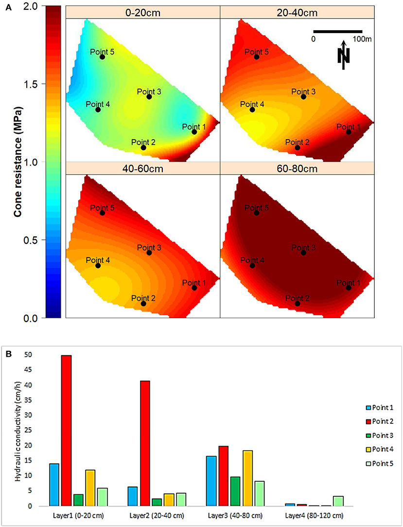
Figure 1. (A) Compaction maps of field S1 showing saturated hydraulic conductivity (Ksat) measurement points. (B) Saturated hydraulic conductivity (Ksat) data measured at different locations in field S1.
HYDRUS-2D requires both the unsaturated hydraulic conductivity and the water retention functions. However, measurement of these variables are expensive, time consuming and impracticable for large scale applications (Pachepsky and Rawls, 2004; Vereecken et al., 2010). Considering the large number of fields and the area covered by this investigation, we decided to define the range of variation (minimum and maximum) of the hydraulic parameters of the soil over the entire study site and to optimize them as needed for each field. Thus, in this article, the hydraulic parameters were optimized on the field S1 and validated on the field S2. Soil sampling for water retention was done at 134 measurement points distributed over the experimental site and were collected during the summer of 2018 at depths of 0–5, 30–35, and 50–55 cm. No water retention measurement was done in layer four (80–120 cm), as soil sampling would have required important excavation. Soil water content was measured for different values of h (ranging from 0 to −1000 cm) using tension tables. The results were used to obtain the general shape of the retention curve for each layer.
Meteorological data included hourly rainfall depth, air temperature, relative humidity, wind speed and solar radiation. These data were collected at the Sainte-Clotilde (Québec) meteorological station (45°9'N, 73°40'W) located about 10 km from the experimental site. Reference evapotranspiration (ETo) was calculated at the hourly time step with the FAO Penman-Monteith formula using the REF-ET software (Allen, 2003) and solar radiation, air temperature, relative humidity and wind speed as input variables. Actual evapotranspiration (ETc) was calculated according to Jensen (1968): ETc = ETo × Kc where Kc is the crop coefficient. Depending on the growth stage, values of Kc for lettuce range from 0.49 to 0.95 (Gallichand et al., 1991). For the stage in which the lettuce was during the measurement period (the end of maturity), we used a Kc value of 0.90.
Drainage System Model Calibration and Validation
HYDRUS-2D (Šimunek et al., 2011) was calibrated with data from field S1 and validated with data from both fields S1 and S2. For model calibration, simulations were done at the hourly scale for a period of 24 h without rainfall on July 16 of 2017 (D37), which corresponded to the end of the lettuce growing cycle during which the canopy covered the entire bed and inter-bed areas. We considered that evaporation from the soil was negligible and that all evapotranspiration was caused by crop transpiration (Allen et al., 1998; Périard et al., 2015).
HYDRUS-2D was used to simulate two-dimensional variably-saturated water flow in a rectangular flow region of 350 cm wide and 120 cm deep, where 350 cm is half of the drain spacing and 120 cm is the simulated soil profile depth, i.e., from the soil surface to the impervious layer. Using a Galerkin-type finite element scheme, HYDRUS numerically solves Richards (1931) equation to which a sink term is added to account for the root water uptake. It represents, per unit time, the volume of water removed from a unit volume of soil due to plant water uptake. The sink term was approximated with Feddes (1978) model whose parameters in histosols were evaluated by Périard et al. (2015): PO = −10.2 cm, POpt = −25.5 cm, P2H = −102.0 cm, P2L = −254.9 cm and P3 = −815.8 cm. The values of r2H and r2L were 0.0369 cm h−1 and 0.0009 cm h−1, respectively, as evaluated from the hourly ETc data as the first quartile for r2L and the third quartile for r2H. Definitions of the Feddes (1978) model parameters can be found in Šimunek et al. (2011).
Several studies carried out in cultivated histosols have shown that for the soil hydraulic parameters evaluation, the van Genuchten-Mualem model (Mualem, 1976; van Genuchten, 1980) fits the observations with satisfying precision (Hallema et al., 2015; Périard et al., 2015; Thériault et al., 2019). The K(h) function was evaluated with the pore-size distribution model of Mualem (1976) using the van Genuchten (1980) retention function. The soil hydraulic parameters θr, θs, α, n, l, and Ksat were optimized during model calibration. Parameters θr and θs are, respectively, the residual and saturation water contents on a volumetric basis expressed in cm3 cm−3. Parameter α, expressed in cm−1, is often described as the inverse of the air-entry. Parameter n is related to the pore-size distribution, and l is the pore connectivity and tortuosity parameter. The soil hydraulic parameters were optimized using the inverse modeling routine of HYDRUS-2D (Šimunek and Hopmans, 2002; Hopmans et al., 2018) which minimizes an objective function (Šimunek et al., 1998) using the Levenberg-Marquardt nonlinear minimization method (Marquardt, 1963). The objective function is based on the difference between observed and predicted h values variations over time.
The range for θs values (0.41–0.94) was obtained from the retention curves at h = 0 of each layer, except layer four (80–120 cm) for which simulations were started using measurements from layer three. The minimum value of θr is usually zero (Šimunek et al., 2011; Périard et al., 2015). For θr maximal value (0.62), we used the maximal water content measurement at h = −1,000 cm. The range for α values (0–0.2) was deducted from Kechavarzi et al. (2010) results for England peatlands (between 0.032 and 0.312) and those of Périard et al. (2015) in Montérégie (between 0.013 and 0.1). Due to Mualem (1976) restriction for reasonable values of m (m = 1–1/n), n was taken as greater than one. For the l value, Mualem (1976) recommends 0.5. The values of Ksat were not optimized by HYDRUS but measured. The initial values for the iterations for each of the parameters were chosen for each layer between the limits indicated above. Since the simulation periods had little or no rainfall, only drainage took place in the soil profile, and it was not relevant to consider hysteresis. The initial conditions used were calculated from a linear distribution of h measured at time t = 0. The boundary conditions were no flux at the sides and bottom of the domain, seepage face at the drain interface, and atmospheric boundary at the soil surface.
For validation, the soil hydraulic parameters obtain during calibration phase were used to predict h. On field S1, the model validation was done on days D1, D2, D5, D23, D24, and D33. On field S2, the model validation was done on day D37. In field S2 pedological description, the Ohp layer 0–40 cm is a homogeneous soil layer. However, comparing the field variations of measured h values over time at depths of 15 and 35 cm showed that the 0–40 cm layer is not hydrologically homogeneous. We, therefore, divided the 40 cm thick Ohp soil layer on S2 into two hydrological layers of 20 cm each allowing h values to be simulated with different α and n hydraulic parameters.
The statistics used to quantify the difference between measured and predicted h values were the Nash-Sutcliffe efficiency coefficient (NSE) (Nash and Sutcliffe, 1970) and the percent bias (PBIAS) (Gupta et al., 1999). The NSE assesses the residual variance proportion relative to the data variance (Nash and Sutcliffe, 1970), and ranges from minus infinity to one. The optimal value is one. PBIAS measures the model tendency to overestimate or underestimate the prediction (Gupta et al., 1999). PBIAS optimal value is zero. We also use the mean absolute error (MAE) and the root mean-square error (RMSE) because they have the advantage of indicating the prediction error in the same unit as h. A MAE or RMSE of zero indicates a perfect fit of the model to the measured h data.
Model Application at Field Scale
To produce vegetables with a high commercial value, the Québec subsurface drainage standard requires a water table drawdown ranging from 30 to 50 cm per day after a rain that saturates the soil profile (h ≈ 0). This is equivalent to a drop in matric potential (Δh) of 30–50 cm at the soil surface. We, therefore, assumed that the objective of a drainage system in a given field was to obtain a minimum value of Δh of 40 cm d−1. Consequently, positive values of Δh correspond to a drawdown of the water table manifested by a drop of the matric potential, and negative values of Δh mean an increase in soil water content and matric potential.
The calibrated/validated model of HYDRUS was used in two different ways. The first model application at field scale was to analyze the effect of compaction on Δh and to identify the optimal combinations of drain spacing and depth to achieve a Δh value of 40 cm d−1. Simulations included drain spacing ranging from 2 to 7 m, with drain depth of either 1 or 1.2 m in five points of field S1. These points were selected to cover all compaction situations of field S1 (Figure 1A). Root water uptake was not considered as it is negligible compared to Δh. The soil profile was initially saturated then left to free drainage. We placed three h observation nodes in the model flow domain, the first near the surface (at 0.05 cm depth), the second at a depth of 60 cm, i.e., below the compact layer, and the last at a depth of 120 cm just above the impervious layer.
The second model application at field scale was to draw response surfaces of Δh to various combinations of layer thickness and Ksat profiles. This analysis was done using data of Point 3 (poor drainage) of S1 field for drain spacings of 2 and 7 m at a drain depth of 1 m. The thickness of the compact layer ranged from 5 to 50 cm centered at a depth of 30 cm below soil surface. Depending on the circumstances, the Ksat values of a peatland may decrease or increase. A decreasing Ksat value might be due to the natural aging of the peat and may affect all four layers of the profile. An increasing Ksat value may be the result of corrective practices made by the producers, like subsoiling, cropping with deep-rooted plants, etc. We assumed that these practices would only affect the two uppermost layers (surface and compact layer). We used maximum Ksat values based on our measurements in the Montérégie region: 591.984 cm h−1 (0–20 cm layer), 1217.7 cm h−1 (20–40 cm layer), 3596.11 cm h−1 (40–80 cm layer), and 25.164 cm h−1 (80–120 cm layer). Since Armstrong and Castle (1999) found a 90% decrease of Ksat over a 25-year drainage period for a peatland, we set the minimum values of Ksat to 5% of the measured values (Ksat Point 3). Therefore, HYDRUS simulations were done with Ksat values going from 5% of actual Ksat to maximal value measured in each layer.
Results and Discussions
Experimental Data
Table 1 presents a summary of the measured data. For both fields, h varied between 30.59 and −327.00 cm and the water table depth varied between 83.65 and 39.30 cm. Throughout the measurement period, the water table remained almost always outside of the root zone (0–40 cm). Analysis of h data showed that 54% of the time, there is no flux in the soil profile (Δh = 0 for all tensiometers). This stagnation time can reach 1 day 23 h (2,820 min, in Table 1). However, in the event of a drop in matric potential (Δh > 0), the rate per 15 min is at least 0.51 cm (Table 1) which would allow a Δh of 40 cm in 19 h 37 min. When evaluated over a day, the range of Δh (Table 2) is higher for h measured at 15 cm deep than at 35 cm showing that h fluctuates more at the soil surface than in the compact layer.
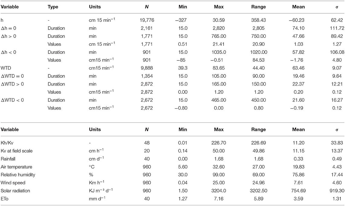
Table 1. Summary of data collected in fields S1 and S2.
Table 2. Matric potential and water table depth variations over a day.
As presented in Table 1, Kh is mostly greater than Kv which is consistent with Beckwith et al. (2003) and Kechavarzi et al. (2010). The Kh/Kv ratio varied between measuring points depths from 0.01 to 226.70. Both ANOVA analysis (at three and four depths) showed that the differences between Kh and Kv were not significant with a p-value of 0.17 (three depths) and 0.46 (four depths). Although the statistical analyses do not show any anisotropy, the high mean of Kh/Kv (11.20 in Table 1) indicates an existing trend toward anisotropy. The fact that no significant statistical difference was found between Kh and Kv may be due to the low number of measurement points used for the anisotropy analysis. However, the absence of anisotropy is consistent with Boelter (1965) and Kechavarzi et al. (2010) and shows the state of advanced degradation of the peatlands. Kechavarzi et al. (2010) reported that the Ksat anisotropy is mainly due to the presence of remains of plant matter causing a horizontal preferential flow in the undecomposed peat. For modeling purposes, we ignored anisotropy and used the geometric mean of Kh and Kv for each measurement point. Measured retention curves are presented in Figures 2A–C. The Ksat measurement points for Δh analysis at field scale are shown in Figure 1A, also showing the state of compaction of the field. The corresponding Ksat values are shown in Figure 1B.
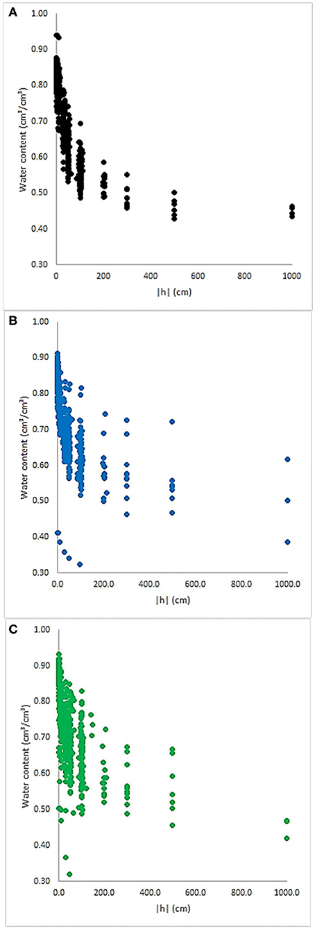
Figure 2. Water retention curves measured at the experimental site on 134 samples collected at (A) 0–5 cm deep, (B) 30-35 cm deep, and (C) 50–55 cm deep.
Calibrated Model Hydraulic Parameters and Validation Results
Calibrated model hydraulic parameters are presented in Table 3 and calibration statistics in Table 4. For calibration in field S1, the NSE value between predicted and observed h values was 0.956 and the PBIAS was −0.57% showing a very low overestimation bias. The retention curves, by layer, after soil hydraulic parameters calibration are presented in Figure 3A. Calibration results are presented in Figure 3B where N1, N2, and N3 are h values modeled corresponding to h values measurement points Obs1, Obs2, and Obs3, respectively. We observed at the soil surface (Obs1 and Obs3) that h measured values increased at 18 and 24 h while there is no precipitation. This could be due to lateral flow from neighboring plots.
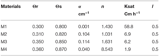
Table 3. Calibrated parameters in field S1.
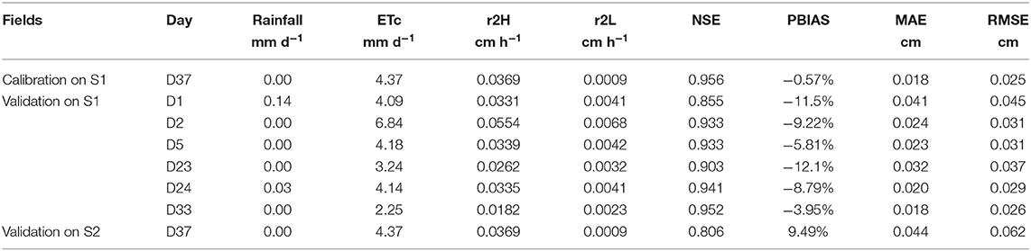
Table 4. Rainfall, ETc. and model calibration and validation results.
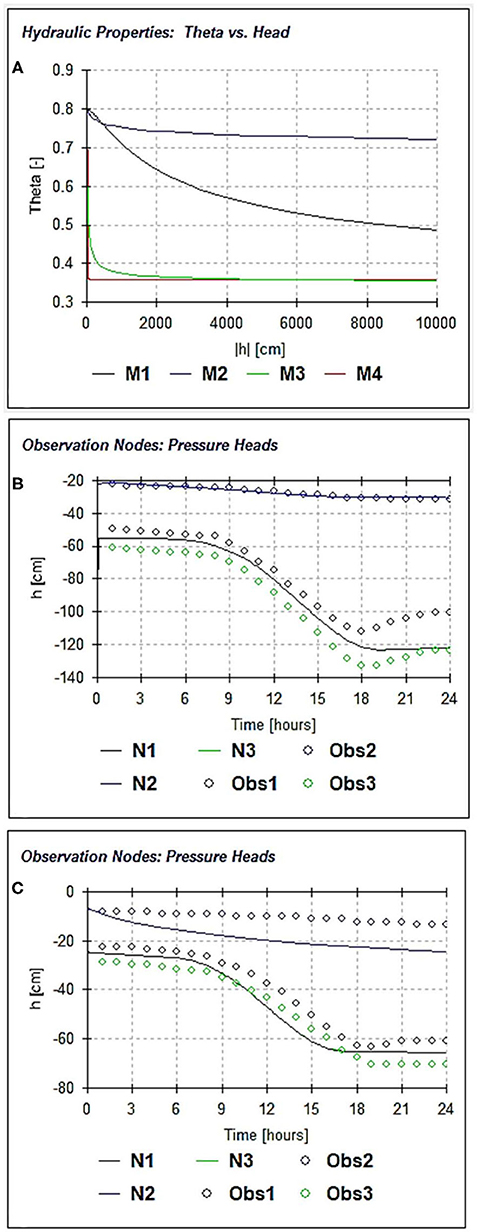
Figure 3. Model calibration and validation results in field S1: (A) Modeled retention curves for material in layer 1 (M1), layer 2 (M2), layer 3 (M3), and layer 4 (M4), (B) Model calibration, (C) Model validation for day D23 for which there is no rainfall. The variables N1, N2, and N3 are h values modeled corresponding to h values measured at Obs1, Obs2, and Obs3, respectively. N3 is hidden by N1. The matric potentials measured at the observation nodes Obs1 and Obs3 are at the same depth and are modeled with the same hydraulic parameters.
Field S1 validation results (Table 4) show high values of NSE (between 0.855 and 0.952) and low values of PBIAS (between −12.13 and −3.95%), MAE (between 0.018 and 0.041 cm) and RMSE (between 0.026 and 0.045 cm) which allowed us to conclude that the model fitted well to the general shape of h variations. On S2, validation results were an NSE of 0.806, a PBIAS of 9.49%. In summary, the statistics of the model calibration and validation confirm that the model is valid. The prediction errors may be due to lateral flows entering as well as leaving the flow domain since the flow domain was not hydraulically isolated during data collection. Another source of prediction errors may be the spatial and temporal variability of the soil hydraulic properties (Schwen et al., 2011; Jirku et al., 2013; Šípek et al., 2019). The pore space in cultivated histosols may be dynamic due to fine particles migration which is almost a continuous phenomenon in Montérégie.
Analysis of Δh
The results of Δh calculations made with HYDRUS-2D are shown in Figures 4A–E. Values of Δh above the compact layer differed from those below the compact layer. Considering all five Ksat measurement points, Δh was on average 58% greater below the compact layer than above it. The smallest differences observed were for Point 2 (16%) and the highest for Point 5 (118%). This implies that the water content above the compact layer does not vary much even if drainage is taking place below the compact layer. For example, for 7 m drain spacing, h values (Figure 5A) and the water flow velocity (Figure 5B) in the soil profile are shown in Figure 5. It allows a better understanding of the water dynamics in each layer. The equipotential lines observation (Figure 5A) shows a slowdown of the water flow inside the compact layer with flow velocities >0.01 cm/h (Figure 5B). The arrangement of the surface layer (high Ksat) and the compact layer (low Ksat) makes the latter a hydraulic barrier favoring water accumulation in the surface layer (Scott, 2000). Indeed, from the soil surface to depth, the infiltration rate decreases to that of the compact layer when the wetting front reaches the interface between the surface layer and the compact layer (Si et al., 2011). In addition, the compact layer inherently has its retention force exacerbated due to the compaction, so the water flow in the compact layer is therefore limited. Contrariwise, the water flow is much faster at depth, particularly in the third layer (Figure 5B) where the drain is located, and where the water accumulation is favored by the low Ksat of the fourth layer. This result confirms the negative impact of compaction on drainage and explains the presence of a perched water table in the fields following heavy rainfalls. For all points, the flow below the compact layer was typical of subsurface drainage with an increase in Δh values as the drain spacing gets smaller.
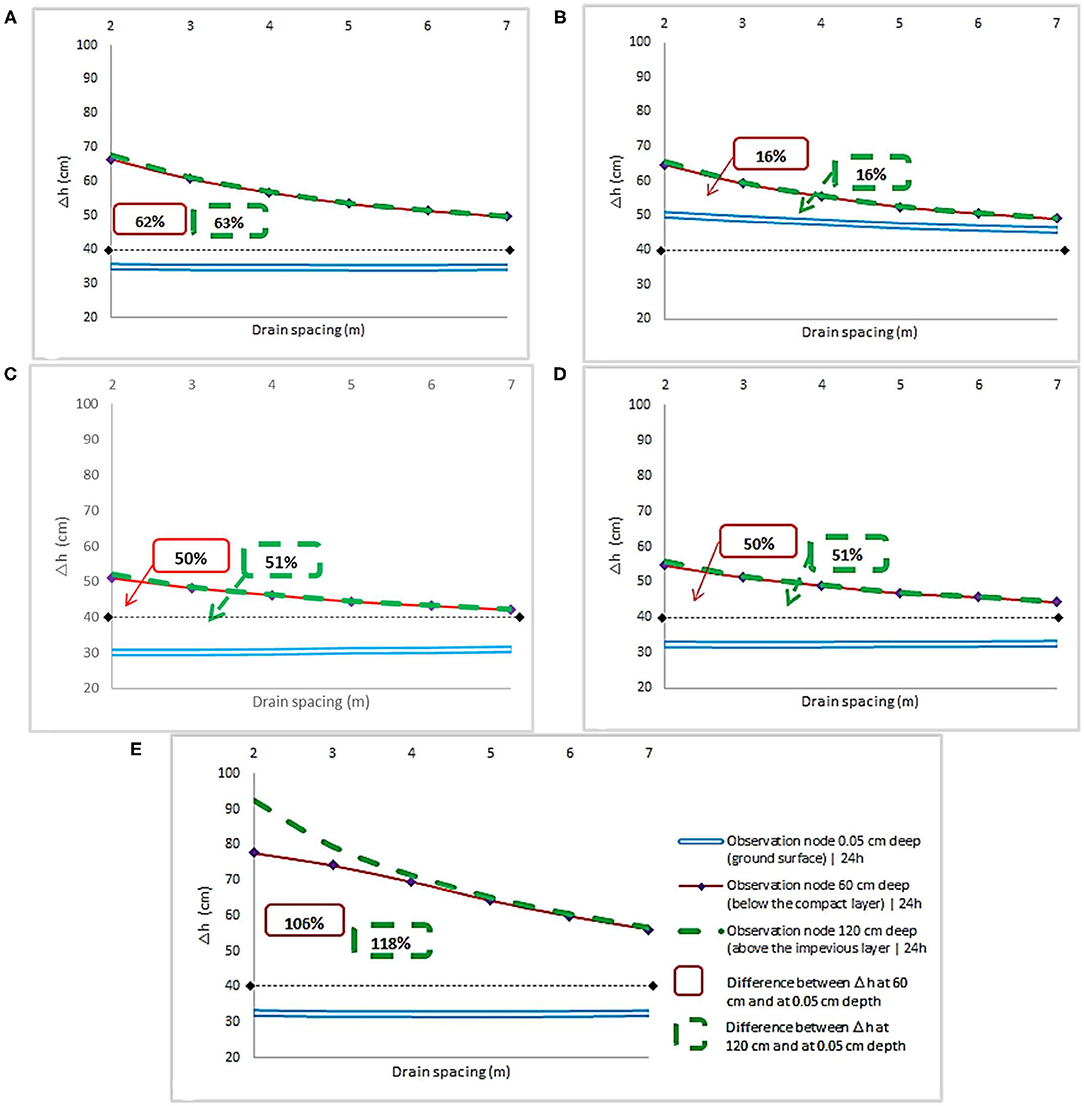
Figure 4. Matric potential variation (Δh) differences between above and below the compact layer for a soil initially saturated and then left in free drainage. The drains are at a depth of 1 m. The observation nodes are at the soil surface, below, and above the compact layer): (A) Point 1; (B) Point 2; (C) Point 3; (D) Point 4; (E) Point 5.
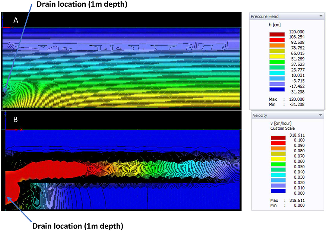
Figure 5. Details of the analysis of the compact layer impact on the subsurface drainage (drain spacing of 7 m and drain at 1 m depth): (A) Matric potential (h) in the flow domain, (B) Water flow velocity toward the drains.
At the soil surface, apart from Point 2 which showed the same trend both above and below the compact layer, the effect of compaction in the other areas is such that it is not relevant recommend a decrease in drain spacing. We can see it in Figures 4A,C–E, Δh does not vary depending on the drain spacing (Observation node at 0.05 cm). These results differ from those of Madani and Brenton (1994) who report an improvement in subsurface drainage and crop yields in a compacted Queen soil for drain spacings of 3 m compared to 12 m. The flow at Point 3 was characteristic of a relatively high compacted soil. Compared to the other Points (Figure 6A), Point 3 presented the lowest Δh at the soil surface corresponding to the worst quality of subsurface drainage in the studied field. Point 2 (the best quality of subsurface drainage) had the highest values of Δh which are 56% higher than those of Point 3. Values of Δh are 14 and 6% higher at Point 1 and at both Points 4 and 5, respectively. Similar results were obtained for drain depth at 1.2 m (Figures 6A,B). The error bars show that as much for a drain spacing of 7 m as of 2 m, the differences between Δh for a drain laid at 1 m deep and that laid at 1.2 m deep are not significantly different. These results showed that it is not relevant to recommend an increase in drain depth.
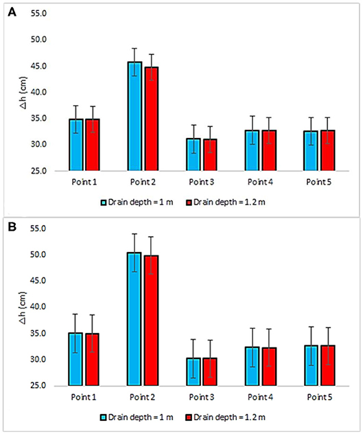
Figure 6. Drop in matric potential (Δh) after 24 h with the drains at a depth of 1 and 1.2 m (soil profile initially saturated and left in free drainage, zero rainfall, observation node located at the soil surface, i.e., 0.05 cm deep): (A) Drain spacing of 7 m; (B) Drain spacing of 2 m.
Optimal Thickness of the Compact Layer and of Saturated Hydraulic Conductivity for Adequate Drainage
Simulated Ksat values are presented in Table 5. Response surfaces of Δh (cm d−1) at the soil surface, as a function of the compact layer thickness and Ksat profiles of Table 5, are presented in Figures 7A,B. Figures 7C,D present the same information for the point below the compacted layer (60 cm deep). Differences in Δh below and just above the impervious layer were practically the same (see Figure 6).
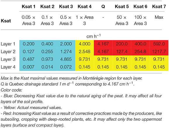
Table 5. Saturated hydraulic conductivity (Ksat) values used for the calculating the Δh response surfaces.
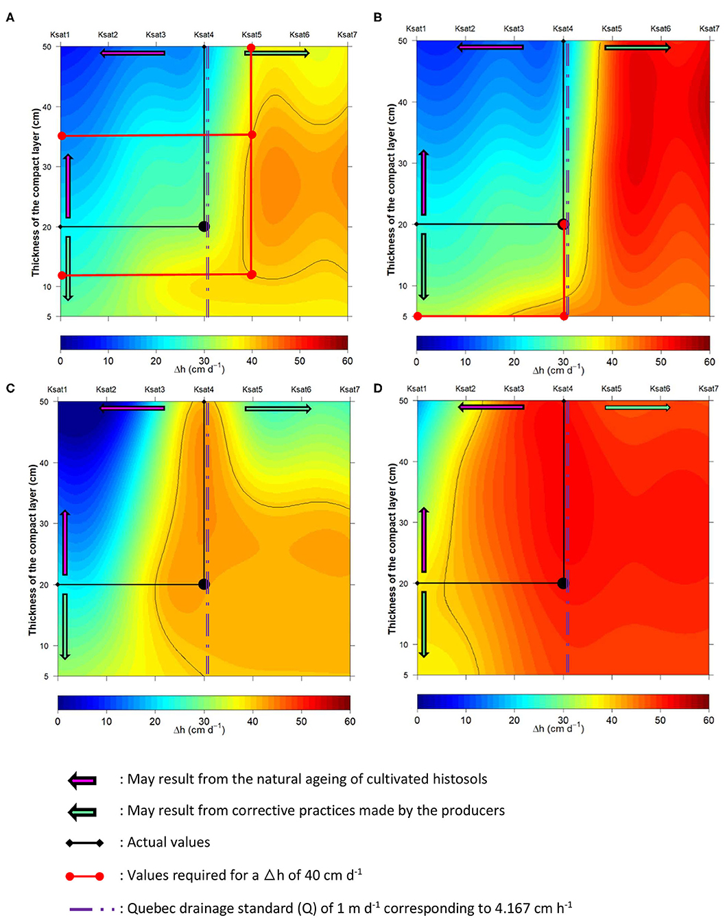
Figure 7. Response surfaces of Δh, in cm d−1, as a function of the compact layer thickness and the Ksat profiles of Table 5. Drain spacing is 7 m (A,C) or 2 m (B,D). Observation point is 0.05 cm (A,B) or 60 cm (C,D) below the soil surface.
The layer dominating the flow would vary depending on the compacted layer thickness and Ksat value of each layer. A Δh of 40 cm d−1 (Figure 7A) would require that the Ksat values in two uppermost layers be multiplied by 50 (Ksat 5 in Table 5) compared to their actual (Ksat 4), and that is valid for compact layer thicknesses between 12 and 35 cm. Outside this region, Δh at the surface is <40 cm and the water content variation within the root zone would be influenced by the difference observed in Δh values above and below the compact layer. The results presented in Figures 7A,C show that if the soil reaches a value of Ksat representing half (Ksat 3) of its actual value (Ksat 4) Δh is <40 cm both at the surface and below the compact layer (Figure 7C). Reducing the spacing to 2 m did not improve Δh at the surface unless the compact layer thickness was reduced to 5 cm (Figure 7B). It can be concluded that for values of Δh ≥40 cm d−1 at the soil surface, the best option should be an improvement of Ksat in the compact layer.
Histosols are known to have a low proportion of conductive pores (Carey et al., 2007). The placement of the surface layer (high Ksat) above the compact layer (low Ksat) makes the latter a hydraulic barrier causing the water accumulation within the surface layer (Scott, 2000). In addition, the compact layer inherently has its retention force exacerbated because of the compaction and of the peat decomposition. Consequently, water percolation through a compact layer is greatly reduced. These results are consistent with those of Smedema (1993), Madani and Brenton (1994) and Alaoui et al. (2011). Madani and Brenton (1994) reported a minimal drain discharge due a compact layer located at a depth varying between 17 and 23 cm deep which extends to bedrock. The recommended solutions relate to the improvement of Ksat in the soil profile and especially in the compact layer. In Montérégie, soil management methods such as subsoiling and cropping with deep-rooted plants are known viable solutions in the short term (Thériault et al., 2019).
Conclusion
Reclaiming peatlands without adequate soil management irreversibly leads to compaction, decomposition and finally to a loss of histosoils. The problem studied in this paper relates to the impacts of peat decomposition and compaction on subsurface drainage. We used HYDRUS-2D to model the drainage system of cultivated histosols in the Montérégie region of Québec, Canada. These soils exhibit a stratification that strongly influences the water flows to the drains. The matric potential variation (Δh) analysis according to different scenarios of subsurface drain spacing and depth showed a difference in Δh values between above and below the compact layer. The drainage was much faster below the compacted layer than above. This analysis also showed that it is not relevant to recommend a modification of drain spacing and depth. An analysis of the thickness of the compact layer and of the hydraulic conductivity required for adequate subsurface drainage showed that, for a Δh of 40 cm d−1, the actual values of hydraulic conductivity in the two uppermost layers should be multiplied by 50 with the thickness of the compact layer varying from 12 to 35 cm. These values can be used as a reference for evaluating the performance of soil management methods such as subsoil or deep-rooted crop to improve Ksat values in the compact layer. Another option is the use of drainage trenches. They could represent a good alternative depending on the material used for the textural continuum, its draining capacity, and its ability to resist clogging.
Data Availability Statement
The raw data supporting the conclusions of this article will be made available by the authors, without undue reservation.
Author Contributions
CG conceived and designed the analysis, collected the data, analysis tools, performed the analysis and wrote the paper. JC conceived and designed the analysis. JG wrote the paper. MB performed the analysis. JD-R collected the data. CL analyzed tools. All authors contributed to the article and approved the submitted version.
Funding
This work was supported by Natural Sciences and Engineering Research Council of Canada.
Conflict of Interest
The authors declare that the research was conducted in the absence of any commercial or financial relationships that could be construed as a potential conflict of interest.
The handling editor declared a past co-authorship with one of the authors (JG).
Acknowledgments
We acknowledge the financial support of the Natural Sciences and Engineering Research Council of Canada (NSERC), Montérégie producers for their practical assistance: Maraîchers J.P.L Guérin et Fils Inc., Vert Nature Inc., Les Fermes Hotte et Van Winden Inc., Productions Horticoles Van Winden Inc., and Delfland. We would like to thank also Dr Steeve Pépin, Dr Guillaume Létourneau, Dr Jonathan Lafond, Alexandre Mc Cutcheon, Sébastien St-Onge, Cyrille Taormina, Raphaël Deragon, Laura Thériault, Renel Lherisson, Diane Bulot, Nicolas Shooner, Josselin Bontemps, Boucar Ly, Abdelali Bouyahia, Camélia Marchand, Gabriel Breton, Joannie Beaupré, Vincent Grégoire, Karolane Bourdon, Mathieu Rémy, Christina Dion, Geneviève Montminy, and Carole Boily who provided extremely helpful assistance both in the field and in the laboratory.
Abbreviations
Δh, matric potential variation; ΔWTD, water table depth variation; D1, D2, …, D40, data collection days from June 27 to July 19 2017; ETc, actual evapotranspiration; ETo, reference evapotranspiration; h, matric potential; K, hydraulic conductivity; Kc, crop coefficient; Kh, horizontal saturated hydraulic conductivity; Ksat, saturated hydraulic conductivity; Kv, vertical saturated hydraulic conductivity; l, pore connectivity and tortuosity parameter; M1, soil first material (Ohp from 0 to 20 cm); M2, soil second material (Ohp compact from 20 to 40 cm); M3, soil third material (Oh from 40 to 80 cm); M4, soil fourth material (Ohp at 0–20 cm); MAE, mean absolut; N1, N2, and N3, h modeled corresponding to Obs1, Obs2, and Obs3, respectively; NSE, Nash-Sutcliffe efficiency coefficient; Obs1, Obs2, Obs3, and Obs4, h measurement points; PBIAS, percent bias; WTD, water table depth, σ, standard deviation; Θr, residual water content; Θs, saturated water content. a, inverse of the air-entry value; n, index parameter related to the pore-size distribution.
References
Alakukku, L. (1996). Persistence of soil compaction due to high axle load traffic. II. Long-term effects on the properties of fine-textured and organic soils. Soil Tillage Res. 37, 223–238. doi: 10.1016/0167-1987(96)01017-3
Alaoui, A., Lipiec, J., and Gerke, H. H. (2011). A review of the changes in the soil pore system due to soil deformation: a hydrodynamic perspective. Soil Tillage Res. 115–116, 1–15. doi: 10.1016/j.still.2011.06.002
Alfnes, E., Kinzelbach, W., and Aagaard, P. (2004). Investigation of hydrogeologic processes in a dipping layer structure: 1. The flow barrier effect. J. Contam. Hydrol. 69, 157–172. doi: 10.1016/j.jconhyd.2003.08.005
Allen, R. G. (2003). REF-ET Reference Evapotranspiration Calculation Software for FAO and ASCE Standardized Equations. University of Idaho, Moscow.
Allen, R. G., Pereira, L. S., Raes, D., and Smith, M. (eds.). (1998). Crop Evapotranspiration: Guidelines for Computing Crop Water Requirements, FAO irrigation and drainage paper. Rome: Food and Agriculture Organization of the United Nations.
Armstrong, A. C., and Castle, D. A. (1999). “Drainage of organic soils,” in Agricultural Drainage (Mansfield), 1083–1105. doi: 10.2134/agronmonogr38.c34
Baden, W., and Egglesmann, R. (1963). Zur durchlässigkeit der moorb∧den. Z. Kultur. Flurber 4, 226–254.
Beckwith, C. W., Baird, A. J., and Heathwaite, A. L. (2003). Anisotropy and depth-related heterogeneity of hydraulic conductivity in a bog peat. I: laboratory measurements. Hydrol. Processes 17, 89–101. doi: 10.1002/hyp.1116
Boelter, D. H. (1965). Hydraulic conductivity of peats. Soil Sci. 100:227. doi: 10.1097/00010694-196510000-00001
Boelter, D. H. (1969). Physical properties of peats as related to degree of decomposition. Soil Sci. Soc. Am. J. 33, 606–609. doi: 10.2136/sssaj1969.03615995003300040033x
Boylan, N., Long, M., and Mathijssen, F. A. J. M. (2011). In situ strength characterisation of peat and organic soil using full-flow penetrometers. Can. Geotech. J. 48, 1085–1099. doi: 10.1139/t11-023
Brandyk, T., Szatylowicz, J., Oleszczuk, R., and Gnatowsk, T. (eds.). (2002). Water-Related Physical Attributes of Organique Soil. Organic Soils and Peat Materials for Sustainable Agriculture. Boca Raton, FL: CRC Press. doi: 10.1201/9781420040098-3
Carey, S. K., Quinton, W. L., and Goeller, N. T. (2007). Field and laboratory estimates of pore size properties and hydraulic characteristics for subarctic organic soils. Hydrol. Processes 21, 2560–2571. doi: 10.1002/hyp.6795
Caron, J., Price, J. S., and Rochefort, L. (2015). Physical properties of organic soil: adapting mineral soil concepts to horticultural growing media and histosol characterization. VZJ 14, 1–14. doi: 10.2136/vzj2014.10.0146
Chapuis, R. P., and Dénes, A. (2008). Écoulement saturé et non saturé de l'eau souterraine vers des drains en aquifère à nappe libre. Can. Geotech. J. 45, 1210–1223. doi: 10.1139/T.07-094
CNRC-NRC (2002). Le système canadien de classification des sols. Ottawa: Agriculture et Agroalimentaire Canada.
Dessureault-Rompré, J., Thériault, L., Guedessou, C.-V., and Caron, J. (2018). Strength and permeability of cultivated histosols characterized by differing degrees of decomposition. Vadose Zone J. 17. doi: 10.2136/vzj2017.08.0156
Duchon, J. (1977). “Splines minimizing rotation-invariant semi-norms in Sobolev spaces,” in Constructive Theory of Functions of Several Variables, Lecture Notes in Mathematics, eds W. Schempp, and K. Zeller (Berlin, Heidelberg: Springer), 85–100. doi: 10.1007/BFb0086566
Eggelsmann, R. (1978). “Subsurface drainage instructions,” International Commission on Irrigation and Drainage, Bulletin. Vol. 6, Deutsches Nationales Komitee; P. Parey.
FAO, (ed.). (1974). Soil Map of The World: Carte mondiale des sols, Vol. 1 [Erl.]: Legend […]. Paris: UNESCO.
FAO (1984). La Conception des réseaux de drainage: 28 questions et réponses : d'après les conclusions de la Consultation d'experts chargée d'examiner les éléments de conception des installations de drainage : Rome, 22–29 octobre 1979. Rome: FAO.
Gallichand, J., Broughton, R. S., Boisvert, J., and Rochette, P. (1991). Simulation of irrigation requirements for major crops in South Western Quebec Can. Agric. Eng. 33, 1–9.
Gupta, H. V., Sorooshian, S., and Yapo, P. O. (1999). Status of automatic calibration for hydrologic models: comparison with multilevel expert calibration. J. Hydrol. Eng. 4, 135–143. doi: 10.1061/(ASCE)1084-0699(1999)4:2(135)
Hallema, D. W., Périard, Y., Lafond, J. A., Gumiere, S. J., and Caron, J. (2015). Characterization of water retention curves for a series of cultivated histosols. Vadose Zone J. 14:vzj2014.10.0148. doi: 10.2136/vzj2014.10.0148
Hopmans, J. W., Šimunek, J., Romano, N., and Durner, W. (2018). “3.6.2. inverse methods,” in Methods of Soil Analysis: Part 4 Physical Methods, 5.4, eds J. H. Dane, and G. Clarke Topp (Chichester: John Wiley and Sons Ltd.), 963–1008. doi: 10.2136/sssabookser5.4.c40
Ilnicki, P., and Zeitz, J. (2003). “Irreversible loss of organic soil functions after reclamation,” in Organic Soils and Peat Materials for Sustainable Agriculture, eds L. E. Parent, and P. Ilnicki (Boca Raton, FL: Taylor & Francis Group). doi: 10.1201/9781420040098.ch2
Jensen, M. E. (1968). “Water consumption by agricultural plants,” in Plant Water Consumption and Response. Water Deficits and Plant Growth, Vol. II, ed Kozlowski, T. T. (New York, NY: Academic Press), 1–22.
Jirku, V., Kodešová, R., Nikodem, A., Mühlhanselová, M., and Žigová, A. (2013). Temporal variability of structure and hydraulic properties of topsoil of three soil types. Geoderma 204–205, 43–58. doi: 10.1016/j.geoderma.2013.03.024
Kechavarzi, C., Dawson, Q., and Leeds-Harrison, P. B. (2010). Physical properties of low-lying agricultural peat soils in England. Geoderma 154, 196–202. doi: 10.1016/j.geoderma.2009.08.018
Lafond, J. A., Bergeron Piette, É., Caron, J., and Théroux Rancourt, G. (2014). Evaluating fluxes in Histosols for water management in lettuce: a comparison of mass balance, evapotranspiration and lysimeter methods. Agric. Water Manag. 135, 73–83. doi: 10.1016/j.agwat.2013.12.016
Lipiec, J., and Hatano, R. (2003). Quantification of compaction effects on soil physical properties and crop growth, Quantifying Agricultural Management Effects on Soil Properties and Processes. Geoderma 116, 107–136. doi: 10.1016/S0016-7061(03)00097-1
Long, M. (2005). Review of peat strength, peat characterisation and constitutive modelling of peat with reference to landslides. Stud. Geotech. Mechanica, Civil Eng. Res. Coll. 27, 67–90.
Lucas, R. E. (1982). Organic Soils (Histosols): Formation, Distribution, Physical and Chemical Properties and Management for Crop Production. East Lansing, MI: Michigan State University, Agricultural Experiment Station.
Madani, A., and Brenton, P. (1994). Effect of drain spacing on subsurface drainage performance in a shallow, slowly permeable soil Can. Agric. Eng. 37, 9–12.
Marquardt, D. W. (1963). An algorithm for least-squares estimation of nonlinear parameters. J. Soc. Ind. Appl. Math. 11, 431–441. doi: 10.1137/0111030
Mathur, S. P., and Levesque, M. (1985). Negative effect of depth on saturated hydraulic conductivity of histosols. Soil Sci. 140, 462–466. doi: 10.1097/00010694-198512000-00010
Millette, J. A., and Vigier, B. (1982). An evaluation of the drainage and subsidence of somme organic soils in Quebec. Can. Agric. Eng. 24, 5–10.
Mualem, Y. (1976). A new model for predicting the hydraulic conductivity of unsaturated porous media. Water Res. Res. 12, 513–522 doi: 10.1029/WR012i003p00513
Nash, J. E., and Sutcliffe, J. V. (1970). River flow forecasting through conceptual models part I—a discussion of principles. J. Hydrol. 10, 282–290. doi: 10.1016/0022-1694(70)90255-6
Okruszko, H., and Ilnicki, P. (eds.). (2003). “The Moorsh horison as quality indicators of reclaimed organic soils,” in Organic Soils and Peat Materials for Sustainable Agriculture (Boca Raton, FL: CRC Press), 1–14 doi: 10.1201/9781420040098-1
Pachepsky, Y., and Rawls, W. J., (eds.). (2004). Development of Pedotransfer Functions in Soil Hydrology, 1st Edn, Vol. 30. Developments in Soil Science Amsterdam, Boston: Elsevier.
Parent (2001). Classification, pédogenèse et dégradation des sols organiques, in: Écologie Des Tourbières Du Québec-Labrador.
Périard, Y., Caron, J., Lafond, J. A., and Jutras, S. (2015). Root water uptake by Romaine Lettuce in a muck soil: linking tip burn to hydric deficit. Vadose Zone J. 14, 1–13. doi: 10.2136/vzj2014.10.0139
Plamondon-Duchesneau, L. (2011). Gestion de l'irrigation des laitues romaines (Lactuca sativa L.) cultivées en sol organique (Mémoire (M.Sc.)). Université Laval, Québec, Canada.
Reynolds, W. D. (2008). “Saturated hydraulic properties: laboratory methods,” in Soil Sampling and Methods of Analysis (Boca Raton, FL: CRC Press), 1013–1024. doi: 10.1201/9781420005271.ch75
Reynolds, W. D., Brown, D. A., Mathur, S. P., and Overend, R. P. (1992). Effect of in-situ gas accumulation on the hydraulic conductivity of peat. Soil Sci. 153, 397–408. doi: 10.1097/00010694-199205000-00007
Richards, L. A. (1931). Capillary conduction of liquids through porous mediums. Physics 1, 318–333. doi: 10.1063/1.1745010
Rycroft, D. W., Williams, D. J. A., and Ingram, H. A. P. (1975). The transmission of water through Peat: I. Review. J. Ecol. 63, 535–556. doi: 10.2307/2258734
Schwen, A., Bodner, G., and Loiskandl, W. (2011). Time-variable soil hydraulic properties in near-surface soil water simulations for different tillage methods. Agric. Water Manag. 99, 42–50. doi: 10.1016/j.agwat.2011.07.020
Scott, H. D. (2000). Soil Physics: Agricultural and Environmental Applications, 1st Edn. Ames: Iowa State University Press.
Si, B., Dyck, M., and Parkin, G. (2011). Flow and transport in layered soils: PREFACE. Can. J. Soil Sci. 91, 127–132. doi: 10.4141/cjss11501
Šimunek, J., Angulo-Jaramillo, R., Schaap, M. G., Vandervaere, J.-P., and van Genuchten, M., Th. (1998). Using an inverse method to estimate the hydraulic properties of crusted soils from tension-disc infiltrometer data. Geoderma 86, 61–81. doi: 10.1016/S0016-7061(98)00035-4
Šimunek, J., and Hopmans, J. W. (2002). “1.7 Parameter optimization and nonlinear fitting,” in Methods of Soil Analysis: Part 4 Physical Methods, 139–157. doi: 10.2136/sssabookser5.4.c7
Šimunek, J., Van Genuchten, M. T., and Sejna, M. (2011). The HYDRUS Software Package for Simulating the Two- and Three-Dimensions Movement of Water, Heat, and Multiple Solutes in Variably-Saturated Media. Springer Reference. Berlin/Heidelberg: Springer-Verlag.
Šípek, V., Jačka, L., Seyedsadr, S., and Trakal, L. (2019). Manifestation of spatial and temporal variability of soil hydraulic properties in the uncultivated Fluvisol and performance of hydrological model. CATENA 182:104119. doi: 10.1016/j.catena.2019.104119
Smedema, L. K. (1993). Drainage performance and soil management. Soil Technol. 6, 183–189. doi: 10.1016/0933-3630(93)90007-2
Smith, C. W., Johnston, M. A., and Lorentz, S. A. (2001). The effect of soil compaction on the water retention characteristics of soils in forest plantations. South Afr. J. Plant Soil 18, 87–97. doi: 10.1080/02571862.2001.10634410
Soil Survey Staff (2015). Illustrated Guide to Soil Taxonomy, Version 2. Washington D. C: United States Department of Agriculture.
Sturges, D. L. (1968). Hydrologic properties of peat from a Wyoming Mountain Bog. Soil Sci. 106, 262–264. doi: 10.1097/00010694-196810000-00003
Thériault, L., Dessureault-Rompré, J., and Caron, J. (2019). Short-term improvement in soil physical properties of cultivated histosols through deep-rooted crop rotation and subsoiling. Agron. J. 111, 2084–2096. doi: 10.2134/agronj2018.04.0281
van Genuchten, M. Th. (1980). A closed-form equation for predicting the hydraulic conductivity of unsaturated soils. Soil Sci. Soc. Am. J. 44:892. doi: 10.2136/sssaj1980.03615995004400050002x
Vereecken, H., Weynants, M., Javaux, M., Pachepsky, Y., Schaap, M. G., and van Genuchten, M. T. (2010). Using pedotransfer functions to estimate the van Genuchten–Mualem soil hydraulic properties: a review. Vadose Zone J. 9, 795–820. doi: 10.2136/vzj2010.0045
Keywords: Peat decomposition, compaction, subsurface drainage, matric potential, HYDRUS-2D
Citation: Guedessou CV, Caron J, Gallichand J, Béliveau M, Dessureault-Rompré J and Libbrecht C (2021) Modeling Subsurface Drainage in Compacted Cultivated Histosols. Front. Water 2:608910. doi: 10.3389/frwa.2020.608910
Received: 22 September 2020; Accepted: 04 December 2020;
Published: 11 January 2021.
Edited by:
Matteo Camporese, University of Padua, ItalyReviewed by:
Wei Shao, Nanjing University of Information Science and Technology, ChinaAndreas Panagopoulos, Institute of Soil and Water Resources (ISWR), Greece
Stefano Ferraris, University of Turin, Italy
Copyright © 2021 Guedessou, Caron, Gallichand, Béliveau, Dessureault-Rompré and Libbrecht. This is an open-access article distributed under the terms of the Creative Commons Attribution License (CC BY). The use, distribution or reproduction in other forums is permitted, provided the original author(s) and the copyright owner(s) are credited and that the original publication in this journal is cited, in accordance with accepted academic practice. No use, distribution or reproduction is permitted which does not comply with these terms.
*Correspondence: Cedrick Victoir Guedessou, Y2Vkcmljay12aWN0b2lyLmd1ZWRlc3NvdS4xQHVsYXZhbC5jYQ==