 Ryan E. Harmon
 Holly R. Barnard
 Frederick D. Day-Lewis
 Deqiang Mao4
 Kamini Singha
- 1Hydrologic Science and Engineering, Colorado School of Mines, Golden, CO, United States
- 2Department of Geography, Institute of Arctic and Alpine Research, University of Colorado, Boulder, CO, United States
- 3Hydrogeophysics Branch, Earth System Processes Division, U.S. Geological Survey, Storrs, CT, United States
- 4School of Civil Engineering, Shandong University, Jinan, China
Internal water storage within trees can be a critical reservoir that helps trees overcome both short- and long-duration environmental stresses. We monitored changes in internal tree water storage in a ponderosa pine on daily and seasonal scales using moisture probes, a dendrometer, and time-lapse electrical resistivity imaging (ERI). These data were used to investigate how patterns of in-tree water storage are affected by changes in sapflow rates, soil moisture, and meteorologic factors such as vapor pressure deficit. Measurements of xylem fluid electrical conductivity were constant in the early growing season while inverted sapwood electrical conductivity steadily increased, suggesting that increases in sapwood electrical conductivity did not result from an increase in xylem fluid electrical conductivity. Seasonal increases in stem electrical conductivity corresponded with seasonal increases in trunk diameter, suggesting that increased electrical conductivity may result from new growth. On the daily scale, changes in inverted sapwood electrical conductivity correspond to changes in sapwood moisture. Wavelet analyses indicated that lag times between inverted electrical conductivity and sapflow increased after storm events, suggesting that as soils wetted, reliance on internal water storage decreased, as did the time required to refill daily deficits in internal water storage. We found short time lags between sapflow and inverted electrical conductivity with dry conditions, when ponderosa pine are known to reduce stomatal conductance to avoid xylem cavitation. A decrease in diel amplitudes of inverted sapwood electrical conductivity during dry periods suggest that the ponderosa pine relied on internal water storage to supplement transpiration demands, but as drought conditions progressed, tree water storage contributions to transpiration decreased. Time-lapse ERI- and wavelet-analysis results highlight the important role internal tree water storage plays in supporting transpiration throughout a day and during periods of declining subsurface moisture.
Introduction
Water potential gradients between the subsurface and the atmosphere control transpiration rates; however, there are physiological mechanisms, such as the use of internal water storage, which trees can use to modify water potential gradients. Water stored internally within a tree is a critical reservoir to avoid consequences of dehydration (Lo Gullo and Salleo, 1992; Cermák et al., 2007; Matheny et al., 2015; Wang et al., 2019), buffer against hydraulic conductivity loss in the xylem and prevent cavitation, and maximize photosynthesis when transpiration exceeds soil water uptake (Zweifel et al., 2005; Verbeeck et al., 2007b). Water can be stored intracellularly within tree tissues or extracellularly under capillary forces in the void spaces between sapwood tissues (Holbrook, 1995). While the contribution of intracellular tree stores to daily water use may be small (<1%) (Cermák et al., 2007), extracellular stores can represent a substantial fraction of daily water use (Tyree and Yang, 1990; Meinzer et al., 2006). The contribution of tree water storage to daily transpiration varies widely across different tree species and ecosystems, ranging from 10 to 50% (Phillips et al., 2003; Cermák et al., 2007), and is not constant from day to day (e.g., Loustau et al., 1996; Zweifel et al., 2005; Verbeeck et al., 2007c). The volume of stored water and reliance on these stores is known to vary with tree size and physiological properties, such as wood density, drought tolerance, and stomatal hydraulic strategy (e.g., isohydric or anisohydric) (Köcher et al., 2013; Matheny et al., 2015). Multiple environmental controls influence tree water storage at any given time—e.g., soil moisture, groundwater elevation, temperature, vapor pressure deficit (VPD), solar radiation— but, which controls have the largest influence has been challenging to isolate. Consequently, given the number of physiologic and environmental factors that can influence the degree to which a tree relies on stored water, it is not surprising that the temporal variability in transpiration and the role tree storage plays in buffering variability in evaporative demand is a current topic of interest (Hartzell et al., 2017; Kaner et al., 2020). Given the inclusion of increasingly complex hydrodynamic processes in tree-level models (e.g., Bohrer et al., 2005; Mirfenderesgi et al., 2016; Huang et al., 2017) there is increased demand for field techniques that can measure (at high spatial and temporal resolutions) the pathways and mechanism driving tree water uptake and transport. Transpiration estimates in many hydrologic models are often guided by empirical relations (e.g., Jarvis et al., 1976; Feddes et al., 2001) that link stomatal conductance directly and instantaneously to measurements of shallow subsurface moisture and VPD, ignoring the role of other variables such as tree water storage (Mirfenderesgi et al., 2016). This model simplification can misrepresent transpiration dynamics at sub-daily time scales because internal water storage can buffer variability in transpiration induced by decreasing subsurface water availability and/or increasing evaporative demand (Matheny et al., 2014; Mirfenderesgi et al., 2016).
The relation between evaporative demand and stomatal conductance has been described by several researchers (e.g., Jarvis and Mcnaughton, 1986; Meinzer, 1993; Ewers et al., 2005; Bunce, 2006); however, the importance of sapwood hydraulic capacity and its potential influence on water potential gradients, which drive changes in stomatal conductance, have received relatively little attention. Several studies have observed a time lag between sapflow measured at the base of a tree and transpiration in the canopy (Landsberg et al., 1976; Goldstein et al., 1998; Phillips et al., 1999; O'Brien et al., 2004); because of internal water storage, transpiration in the canopy can start several minutes to hours before water starts to flow at the base of the stem (Schulze et al., 1985; Steppe and Lemeur, 2004). Longer time lags have been observed in larger trees with greater storage capacity (e.g., Goldstein et al., 1998), but as capacitance in stems decreases, lag times decrease as steepening water potential gradients between the canopy and base of the stem are not abated by water released from storage (McCulloh et al., 2019).
Tree water storage remains a challenging variable to estimate in the field (Burgess and Dawson, 2008; Phillips et al., 2009; McCulloh et al., 2019). It seems likely that some of the observed variability in volume of water contributed from internal storage to transpiration may result from the different field techniques that have been employed to measure changes in tree water storage. Internal tree water storage has been measured by tree coring (Borchert, 1994; Scholz et al., 2007), digital dendrometers (Köcher et al., 2013; Cocozza et al., 2015), networks of sapflux sensors (Goldstein et al., 1998; Phillips et al., 2009), and time-domain and frequency-domain reflectometry (TDR and FDR) (Wullschleger et al., 1996; Matheny et al., 2015). Each method has unique measurement sensitivities and support volumes, as well as advantages and disadvantages; however, a common weakness that applies to each of these methods, with the exception of the dendrometer, is that measurements are made at a point within the tree. Consequently, there has been increasing interest in electrical resistivity imaging (ERI) to explore the internal properties of trees (Al Hagrey, 2007; Bieker and Rust, 2010; Lin et al., 2012; Guyot et al., 2013; Wang et al., 2016; Benson et al., 2019). ERI is a non-destructive measurement technique that images spatial and temporal variations in bulk electrical conductivity (the reciprocal of bulk electrical resistivity)—a property that can be linked to water moisture inside a tree (e.g., Ganthaler et al., 2019; Carrière et al., 2020). Electrical impedance tomography has also been used successfully to explore the internal properties of trees (e.g., Martin, 2012; Martin et al., 2015; Kessouri et al., 2019). Mares et al. (2016) used ERI to map diel cycles in bulk electrical conductivity in a tree trunk, potentially caused by the emptying and refilling of stored water within the tree; Luo et al. (2020) expanded on this work by developing an empirical electrical conductivity-based method to estimate stem water content. However, quantitatively estimating tree moisture content with ERI is challenging because the relation between electrical conductivity and moisture content is influenced by variables such as temperature, solute concentration, and material properties (e.g., Day-Lewis et al., 2005; Garré et al., 2013; Luo et al., 2019). In a tree, the measured electrical conductivity may also be sensitive to cell structure, which varies among tree species and is distinctly different in hard vs. soft woods (Repo, 1988; Al Hagrey, 2007; Luo et al., 2019). While trunk electrical conductivity is likely most sensitive to changes in moisture and temperature (e.g., Ganthaler et al., 2019; Luo et al., 2019), the influence of changes in ionic concentrations in the trunk is unknown because measurements of sapwood concentration are difficult to collect in most species due to the tension under which xylem water is held.
In this work, we look to quantify and isolate environmental and physiological controls of internal tree moisture with ERI by collecting these data with multiple corroboratory in-tree measurements, including moisture via FDR, sapflow, a dendrometer, and xylem fluid electrical conductivity, as well as properties of the soil and micrometeorology. We explore time lags among these datasets to infer processes; time lags have previously been used to determine which meteorological variable (e.g., solar radiation, temperature, or VPD) has the strongest influence on sapflow at sub-daily to seasonal timescales (Phillips et al., 1999; Sevanto et al., 2002; Oguntunde, 2005; Hong et al., 2019; Zhang et al., 2019). These studies used cross-correlation to determine the time lag between sapflow and a meteorologic variable. Cross-correlation analyses can be limited because they require stationarity and the frequency of interest (i.e., daily frequencies) is not isolated, thus lags calculated at the frequency of interest can be influenced by other frequency components. More often than not, hydrologic and ecologic data are not stationary due to the influence of episodic events and seasonal trends. Here, we use wavelet analysis—a tool used to characterize the frequency content of a signal as a function of time—which offers three main advantages over cross-correlation analyses: (1) episodic data and seasonal trends can be included because stationarity is not a requirement, (2) correlations can be isolated to specific frequencies associated with controlling processes, and (3) correlations can be confined to certain temporal windows, when the controlling processes are in effect. Because of these advantages relative to conventional spectral analysis and cross correlation, wavelet techniques have been applied to a number of questions in hydrology (Henderson et al., 2009; Pidlisecky and Knight, 2011; Yu and Lin, 2015; Arora et al., 2016; Wallace et al., 2019). To the best of our knowledge, wavelet analysis has not been utilized to explore temporal relations between transpiration and subsurface and tree water stores. Ultimately, we look to show that ERI measurements of internal tree moisture, in conjunction with corroboratory measurements and time-series data exploration techniques, can link tree water-storage patterns with environmental and physiological drivers.
Field Site
Data were collected on and in the proximity of a ponderosa pine (Pinus ponderosa) tree located on south-facing aspect (40°0′45.259″N, 105°27′41.914″W) of the Gordon Gulch watershed within the Boulder Creek Critical Zone Observatory (BCCZO), which lies within the Arapahoe National Forest in the Colorado Front Range, Colorado, USA (Figure 1A). Ponderosa pine are known to have deep sapwood, which increases bole storage capacities (Domec et al., 2005). The Gordon Gulch watershed is 2.6 km2, ranges in elevation from 2,435 to 2,732 m, and lies within a montane climatic zone. Average annual precipitation is ~530 mm with ~40% falling as snow, 40% as rain, and the remaining 20% as a mix of the two (Cowie et al., 2017). The south-facing slopes of Gordon Gulch are dominated by ponderosa pines, while north-facing slopes are densely vegetated with lodgepole pine (Pinus contorta) (Figure 1A). In the lower reach of Gordon Gulch, the average stand density of ponderosa pine forest is ~600 trees/ha, which is equivalent to one tree within every 4 m2 (Mares et al., 2016). Soil depth was determined during our excavation of three soil pits surrounding the ponderosa pine and ranged from 30 to 40-cm (Figure 1B). The soils are characterized as typic haplustolls and vary in composition with depth (Mares et al., 2016). Soils are underlain by highly weathered rock that ranges from 5 to 7 m in depth (Befus et al., 2011). Depth to groundwater was not available near our study tree; however, three deep wells in the upper reach of Gordon Gulch have groundwater depths that range from 5 to 11 m below the ground surface, depending on the time of year and position along the hillslope.
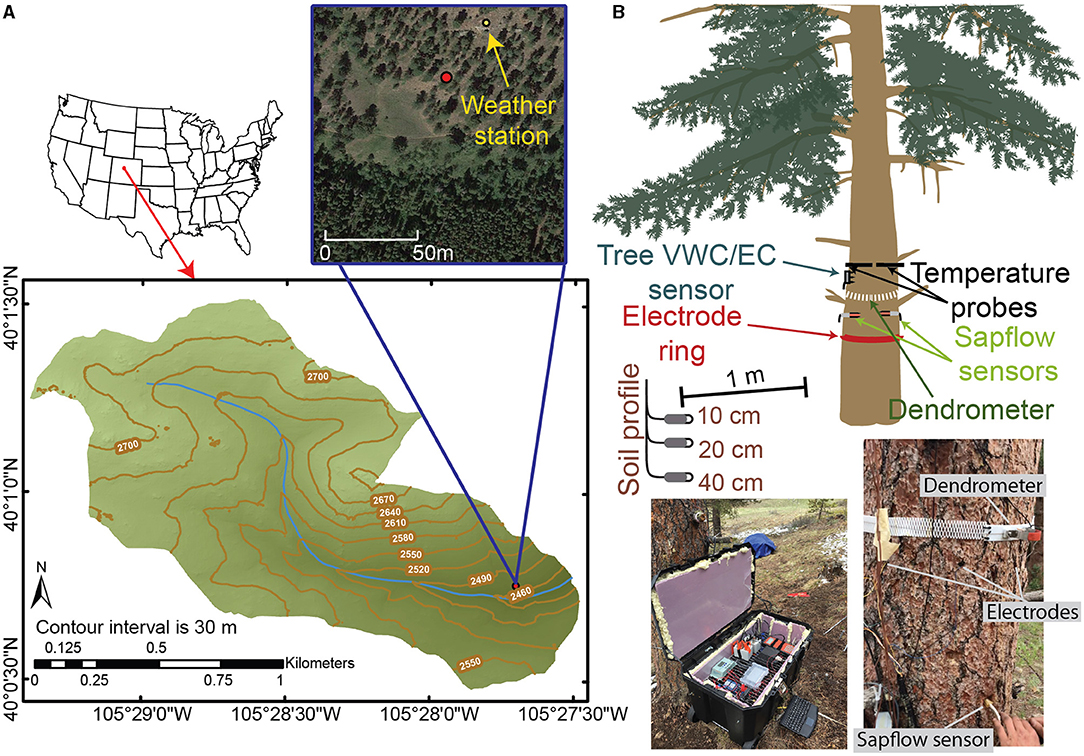
Figure 1. (A) Map of the Gordon Gulch watershed with an aerial image of the location of our study tree (red dot). (B) A schematic of the study tree and the locations of the various instruments installed and pictures showing some of the instrumentation.
Methods
To assess the relations between tree water storage and environmental factors, we collected a variety of data through time during the 2018 growing season, from June 1 to November 1. Soil moisture and meteorological data were measured to describe how environmental changes affected the hydraulic status of the ponderosa pine as inferred by a variety of in-tree measurements (Figure 1B). Dendrometer and ERI measurements were collected to estimate radial changes in tree moisture. To account for the effects of temperature on ERI measurements, temperature data were collected within a cross-section of the tree trunk. Two pine dowels with embedded thermistors were inserted into the north and south faces of the tree trunk 1 m above the ground surface (Figure 1B) such that a temperature profile through the trunk of the tree could be measured. Temperature measurements were made at 2, 10, 22, 26.5, 34, 38, 42, and 46 cm across the north to south profile (tree diameter = 47.5 cm at time of installation). Additionally, to account for the potential effects that changes in electrical fluid conductivity could have on ERI, we sampled the fluid electrical conductivity of water within sapwood cores of neighboring ponderosa pines through the growing season. A 3-D terrestrial laser scan of the ponderosa pine tree was conducted using Leica ScanStation C10 (https://w3.leica-geosystems.com/) to determine tree height (~13 m), maximum crown diameter (~6 m), and to precisely locate the positions where ERI electrodes were emplaced into the tree. The closest neighboring tree is 5 m southeast of the study tree.
Meteorological Data
Meteorological conditions have been continuously monitored since 2012 at two stations in Gordon Gulch (https://www.hydroshare.org/group/140). Relative humidity, air temperature, incoming shortwave radiation, and precipitation data, measured at 5-min intervals, were acquired from the south-facing meteorological station (Figure 1A). Meteorological conditions were also measured using a Decagon Microclimate Monitoring System (relative humidity, temperature, wind speed, precipitation, and incoming solar radiation) during the 2018 growing season in an open meadow ~70-m upslope of the study tree at 30-min frequency. Temperature and relative humidity were used to calculate VPD at both stations; however, the relative humidity sensor at the station immediately upslope of the study tree did not function correctly. Thus, VPD from the south-facing meteorological station was used in our analyses. Days with a daily mean VPD within the lowest 33% percentile of the VPD recorded over the study period were considered “low VPD” days, while days within the highest 33% percentile were considered “high VPD,” and days within the inner quantile were considered to have “intermediate VPD” conditions (Matheny et al., 2014); this partitioning of VPD days is used to parse periods of high evaporative demand from periods with little demand.
Soil Moisture Data
Soil volumetric water content (VWC) was measured at three locations around the study tree with METER ECH2O EC-5 sensors (https://www.metergroup.com/environment/products/ec-5-soil-moisture-sensor/). In soil moisture profiles one and three, sensors were installed at 10 and 30-cm depth. Profile one was located 3-m northwest of the study tree, while profile three was located 3-m to the southwest of the study tree. In profile two, which was located 1-m to the west of the study two sensors were installed at 20 and 40-cm depth. All sensors were installed in January 2018 and recorded data every 30 min until November 1. Soil sensors were not calibrated to the site-specific soil type because we were interested only in relative changes through time. The multiple linear regression technique developed by Cobos and Campbell (2007) was used to temperature correct soil VWC measurements.
Tree Electrical Conductivity Data
Dipole-dipole ERI surveys with a maximum spacing between current and potential electrodes using four electrodes were continuously recorded every 3 h from June 1 to November 1 using a Lippmann 4-point light 10 W resistivity meter (https://www.l-gm.de/en/en_resistivity.html). We attempted to collect data for an entire year during this study, but did run into power supply issues and increased contact resistances resulting from the tree trunk freezing during the wintertime. Stainless-steel wood screws (5 mm in diameter and 2.5 cm in length) were used as electrodes. Screws were driven 2 cm into the xylem of the study tree in June 2017, 1 year prior to our study period, to reduce the potential effects of the tree-healing response on electrical conductivity measurements. A total of 224 quadrupoles were measured in each ERI survey, which took ~0.5 h to collect. Sixteen electrodes were evenly spaced 7-cm apart and formed a level ring that encircled the trunk. Contact resistances between the screws and the tree were generally around 40 kΩ. Stacking errors, which is a measure the repeatability of an individual measurement, were <5% in 90% of the data collected. Twenty quadrupoles had large stacking errors (20%) throughout the study period and were consequently removed from the time-lapse ERI inversion analysis. Reciprocal errors are used to compare differences associated with the directionality of the measurement and are measured by switching the current and potential electrode pairs (Parsekian et al., 2017). By the principle of reciprocity, the measurements should be equal, thus any difference is considered to indicate a measurement error (Habberjam, 1967). Reciprocal measurements were acquired immediately after each ERI survey. The median reciprocal error for all surveys was 1.4% with a standard deviation of 15%. Reciprocal and stacking errors remained mostly constant through time, with the exception of: (1) a couple of days that corresponded to large storm events, which likely saturated the bark and changed the contact resistances, and (2) data collected after mid-September when noise levels in the ERI data increased drastically.
Resistances measured in each ERI survey were inverted using a code developed in COMSOL Multiphysics (Mares et al., 2016). The inversion is based on a regularized objective function combined with weighted least squares:
The 2.5D inversion simulates current in 3D, but calculates 2D log10 resistivity distributions on a domain that is assumed to extend uniformly into the third dimension (e.g., Dey and Morrison, 1979). The m is the model vector of resistivities (inverse of electrical conductivities); d is the measured resistance data; Wd is the data-weighting matrix based on reciprocals of the measurement errors, where all values were considered equal in this case (e.g., all values in the data-weighting matrix were set to one); f(m) is the forward solution of the modeled resistances; Wm is the model-weighting matrix based on a second-derivative filter that acts as a smoother during minimization of the objective function; β is a tradeoff parameter that is modified upon each iteration during the optimization to balance the data misfit (first term on right-hand side of equation) and model smoothing (second term on the right-hand side of the equation); and mref is the starting model, which is homogenous (set at 500 Ωm—the average apparent resistivity of the surveys during the study period) in the temperature-correction inversions described in the following paragraph and inhomogeneous in time-lapse inversions. The inversion mesh was made of 518 triangular elements, which were further divided into four smaller triangular elements in the forward mesh for finer discretization of the forward problem. A model resolution matrix R was used to assess areas of the model that were well-constrained by the data, and was calculated after each inversion:
where J is the Jacobian matrix which contains the sensitivities of the measurements with respect to the model parameters.
ERI data were corrected for temperature prior to the time-lapse inversions following Hayley et al. (2010) method, which suggests that before time-lapse inversion, each ERI survey should be inverted independently and the resulting electrical conductivity model corrected for temperature using an established relation between temperature and electrical conductivity. The forward solution of the temperature-corrected conductivity models can then be calculated, yielding the bulk apparent conductivity at the standard reference temperature (i.e., the temperature-corrected ERI data). Luo et al. (2019) investigated the relation between temperature changes in tree trunks and electrical conductivity and found that the relation can be accounted for using an exponential temperature correction model:
where σm is the inverted pixel conductivity at the measurement temperature (T), σref is the conductivity at a standard reference temperature (Tref), which was set to 25°C in this study, and α is a fitting parameter. A cross-sectional temperature profile of the tree trunk was estimated by linearly interpolating across the eight-temperature measurements. All pixel temperatures were extrapolated from the cross-sectional temperature profile. For the temperature-correction model, we assumed alpha was −0.034°C−1 as suggested by Luo et al. (2019) for sapwood in a living tree. The time-lapse inversions (e.g., the difference between mref and the inversion result at a later time) were then performed using the temperature-corrected data and the COMSOL Multiphysics code, and the mref was set to the temperature-corrected inversion result for June 1 at 0130 h, which was considered time zero.
To examine temporal trends in trunk bulk electrical conductivity, the median bulk electrical conductivity of each temperature-corrected inverse model was calculated; however, because the heartwood plays a minor role in diel and seasonal tree hydraulics relative to the sapwood (e.g., Cermák et al., 2007), we removed the estimated heartwood region from the median calculation. Six tree cores were extracted at the end of the field study to determine the location of the heartwood/sapwood boundary. An ellipse was fit to the six points to approximate the spatial extent of the heartwood for this purpose. Regions of the inverse models where the resolution was poor (i.e., within the lowest 25 percentile) were also removed from the median calculation; these regions largely overlapped with the heartwood. After removal of these regions, the median inverted electrical conductivity was interpolated to 30-min time steps using a spline function in Matlab so that all time-series data could be analyzed using a uniform timestep, which is required by the cross-wavelet code. In the following discussion, we refer to the interpolated median of the inverted sapwood electrical conductivity as the inverted sapwood electrical conductivity.
Other In-tree Measurements
A number of corroboratory measurements were made to interpret the inverted sapwood electrical conductivity. A METER TEROS 12 frequency-domain reflectometry sensor (https://www.metergroup.com/environment/products/teros-12/) was inserted into the xylem 2 m above the ground surface, which provided an indirect measure of VWC and measured temperature every 30 min. Few studies have employed FDR sensors for the purpose of measuring in-situ stem-water content. Existing examples include a few subtropical species (Holbrook et al., 1992; Oliva Carrasco et al., 2015) and deciduous trees with relatively high wood densities when compared to pine, e.g., a red maple (Matheny et al., 2015) and birch (Hao et al., 2013). To our knowledge, the only pine species that has been monitored with a FDR sensor is a white pine instrumented by Matheny et al. (2017); however, because the purpose of their study was to introduce a tree-specific protocol for calibrating and installing FDR sensors, detailed analysis of their field measurements were not presented. The TEROS 12 FDR sensor was not calibrated because we were interested in relative changes through time; VWC estimates using the default soils calibration are unlikely to be representative of the true VWC of the ponderosa pine's xylem. Given that lower-density trees like pines generally have a larger hydraulic capacitance (Oliva Carrasco et al., 2015) and isohydric species have been shown to be more reliant on stored water (Matheny et al., 2015), we expected to measure large, clear diel fluctuations in sapwood moisture in the ponderosa pine tree.
Heat-pulse ratio sapflow sensors (Burgess et al., 2001) were installed at 1.5 m above ground surface on the east and west sides of the study tree (Figure 1B), and data were recorded every 30 min. A METER digital dendrometer (https://www.metergroup.com/environment/#d6), which measures changes in the circumference of a trunk, was attached 50-cm above the electrode ring and collected data every 30 min. Variations in stem diameter result from: (1) irreversible radial stem growth and (2) reversible stem shrinking and swelling caused by dynamics in water storage (Zweifel et al., 2001; Oberhuber et al., 2020).
To determine if changes in ionic concentrations contribute to seasonal and diel changes in measured bulk electrical conductivities, xylem water was sampled by coring into the xylem of nearby ponderosa pines. Because coring is invasive, we avoided coring the study tree during the study period. To extract water from tree cores, the phloem and bark were removed from the cores and then water was squeezed out of the remaining cores using a 12-ton shop press. Squeezing may mobilize constituents that are not freely flowing within the xylem; however, squeezing provided the best practical proxy for changes in xylem osmolytes. Fluid electrical conductivity was subsequently measured from the extracted fluids using a Mettler Toledo benchtop electrical conductivity meter.
Wavelet Analysis
We used the continuous wavelet transform (CWT), the cross wavelet transform (XWT), and wavelet coherence (WTC) to transform pairs of time series (tree water storage vs. solar radiation, VPD, sapflow, and soil moisture (e.g., Figure 2A) into the time-frequency domain so that correlations between pairs can be (1) isolated to specific frequencies associated with controlling processes, and (2) confined to certain temporal windows, such as stormy periods (for more detail on cross wavelet transforms see Kumar and Foufoula-Georgiou, 1997; Torrence and Compo, 1998; Grinsted et al., 2004). In the CWT, a wavelet—a unit-energy signal localized in time and frequency—is scaled and dilated to identify frequency components of a dataset at a specific point in time (Figure 2B). This process identifies frequencies in the data that are driven by a reoccurring process. The CWT cannot simultaneously accomplish high resolution in both time and frequency because low-frequency components are resolved by stretching and downscaling wavelets, which leads to lower temporal resolution; conversely high-frequency components are identified by shrinking and scaling wavelets and thus are resolved well in time, but not in frequency (Torrence and Compo, 1998). At moderate frequencies (i.e., frequencies that are not near the frequency limits of the data set based on the measurement time step and length of the data collection period), the CWT can successfully localize time–frequency representations of time-series data, and thus can isolate non-stationary frequency patterns within time series. The frequencies of interest in this study (e.g., daily) fall within the moderate frequency range. The CWT of a time series is:
where is the transformed times series for scale s (e.g., 1.5 h to 32 days in this study), t is the uniform time step of the time-series data, n is an integer value used to shift the wavelet used (n = 1,. . .,N; where N the number of time steps), n′ is a reversed time shift (N,. . ., n = 1), and is the original time-series data. In this study, the XWT and CWT deconstructed time series data into frequencies that ranged from 1.5 h to 32 days; however, we focus on the 1-day frequency to determine how tree water storage affects the diurnal pattern of water use. There are a number of wavelet functions (ψ0) that can be used in the CWT, each with advantages and disadvantages; for our purpose, the commonly applied Morlet wave was selected because the properties of the wavelet enable the separation of phase and amplitude components associated with a signal (Addison, 2018). The Morlet wavelet function is defined by:
where ω0 is dimensionless frequency and η is dimensionless time, which depend on the measurement time step and data collection period, respectively. Phase information can be extracted using the Morlet CWT and the XWT, which is used to infer power between the two time series (here called X and Y) by multiplying the real portion of the CWT of X and the complex conjugate of the CWT of Y (e.g., Figure 2C):
where WX is the real portion of the CWT of X and WY* is the complex conjugate of the CWT of Y and wavelet power is calculated by |WXY|2 (Figures 2B,C). This cross-wavelet power spectrum is important because it shows the temporal relations (e.g., phase offset) between two time series across different timescales.
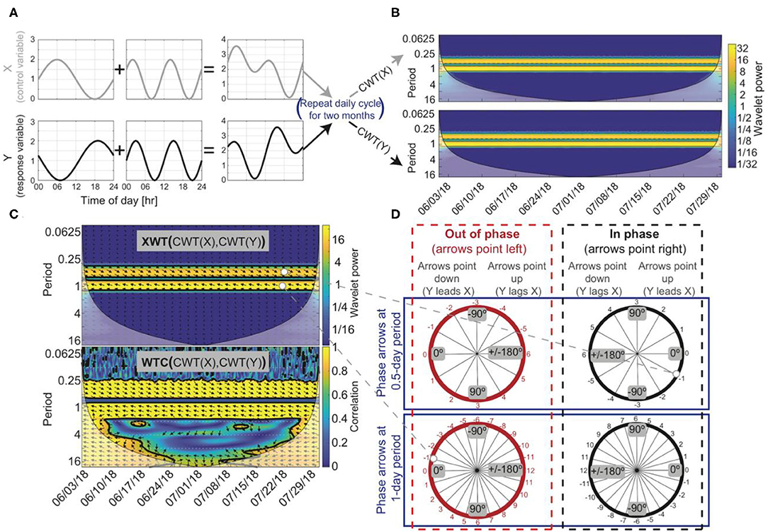
Figure 2. An example of how to test for temporal relations using wavelet analysis, assuming two hypothetical time series, X and Y, that span June 1–July 31, 2018, where changes in X drive changes in Y. (A) X is the summation of a sine wave with a 1-day period and a sine wave with a 0.5-day period. Y is the summation of a cosine wave with a 1-day period and a sine wave with a 0.5-day period. The cosine wave and sine wave that make up Y were both shifted forward by 1 h so that Y lagged X at the 0.5 and 1-day periods. (B) The continuous wavelet transforms (CWT) of X and Y indicates that both are composed of reoccurring cycles with a 0.5 and 1-day periods. (C) The cross-wavelet transform (XWT) also identifies the high power at the 0.5 and 1-day periods, and the wavelet coherence method (WTC) indicates X and Y are highly correlated around the 0.5 and 1-day periods. Arrows at the 0.5 and 1-day period are phase locked, meaning X's influence on Y is constant through time, suggesting a causal relationship between X and Y is likely. (D) Arrows indicate a phase angle of −30° at the 0.5-day period with Y lagging X by 1 h and a phase angle of 15° at the 1-day period with Y lagging X by 1 h. Arrows that point to the left suggest that X and Y are out of phase (red circles) and phase arrows that point to the right suggest X and Y are in phase (black circles). However, visual inspection or some physical process knowledge about X and Y is needed to confirm the phase relation between X and Y because phase can be misinterpreted at longer lag/lead times (i.e., phase arrows at a 1-day period may indicate that X and Y are out of phase with Y lagging X by 1 h or that X and Y are in phase with Y leading X by 1 h). In this hypothetical example, X and Y are out of phase at the 1-day period with Y lagging X by 1 h, suggesting a negative correlation and that a change in X causes a change in Y 1 h later. At a 0.5-day period, X and Y are in phase with Y lagging X by 1 h, suggesting a positive correlation with a 1-h delay.
The XWT identifies regions within the CWTs where there is high power between two time series (Figure 2C). When there is high power there may be a causal relationship between the two time-series datasets. However, misleading results in the XWT can appear when high power is calculated in one of the CWT transforms but not the other because the power calculated in the CWTs are not normalized prior to the calculation of the XWT (Maraun and Kurths, 2004; Yu and Lin, 2015). This limitation of the XWT can be overcome with the WTC, in which the cross-wavelet power |WXY|2 is normalized by the product of the individual CWTs (Yu and Lin, 2015; Figure 2C). For the WTC equation, see Torrence and Webster (1998). The WTC can be thought of as the correlation between the two time series in frequency space (Grinsted et al., 2004); thus, high-power phase relations in the XWT that coincide with regions of high correlation in WTC can be considered statistically significant. Note that the disadvantage of the WTC method is that it is less localized in time-frequency space (Figure 2C); thus, to assess relations among X and Y the XWT and WTC method should be used together. If phase arrows are constant or vary slightly through time in the WTC at a specific period, then a causal relation between X and Y is likely. In short, the CWT transforms a time series into the time-frequency domain, the XWT computes phase relations between two CWTs, and the WTC identifies areas in time-frequency space where there is significant correlation between two CWTs.
The CWT is calculated to transform data into time-frequency space. The XWT and WTC are used to determine causal relations between the assumed driving variables X (i.e., sapflow, soil moisture, VPD, net radiation) and the response variable Y (e.g., inverted sapwood electrical conductivity measured in the ponderosa pine) (illustrated using black arrows in Figure 2C). Phase angles between X and Y were used to calculate lag times (Grinsted et al., 2004):
where Δt is the lag time, Δϕ is the phase angle in radians, and T is the period under consideration (e.g., if diel fluctuations are the focus, a 1-day period would be used) (Figure 2D). If we calculated a positive lag time, indicating that a change in Y (e.g., inverted sapwood electrical conductivity) leads a change in X, we concluded that there is no causal relation because X drives changes in sapwood conductivity, not the opposite.
Field Results and Discussion
Soil Moisture
Soil moisture generally declined from the June 1 to late August (Figure 3A). Large rain events led to increases in soil moisture sensors at 10-cm depth, but did not always lead to large increases in the deeper sensors. It is not clear why the storm events in July only caused a muted response in the 20 and 30-cm sensors in profile two, while the storm event in early September led to a substantial increase in moisture at depth. A similar behavior was noted in soil profile one, the large storm event in the latter part of July led to a substantial increase in soil moisture at 30-cm depth, but the early September did not lead to an increase in moisture. Diel fluctuations in soil moisture at 20 and 40 cm were apparent in soil profile two during dry periods following rain events (Figure 3A). After temperature correction, diel fluctuations in soil moisture were above the absolute error (±0.03 m3/m3) reported by METER, and the magnitude of the fluctuations was greater than the measurement resolution of these sensors (0.001 m3/m3); however, the time of daily maxima and minima in soil moisture could not be well-constrained because gradual changes occurring within the 30-min timestep were often smaller than the measurement resolution of the sensor. Diel fluctuations measured in 10-cm sensors in profiles one and three were strongly influenced by temperature, consequently, an evaporation/transpiration signal could not be parsed from these data.
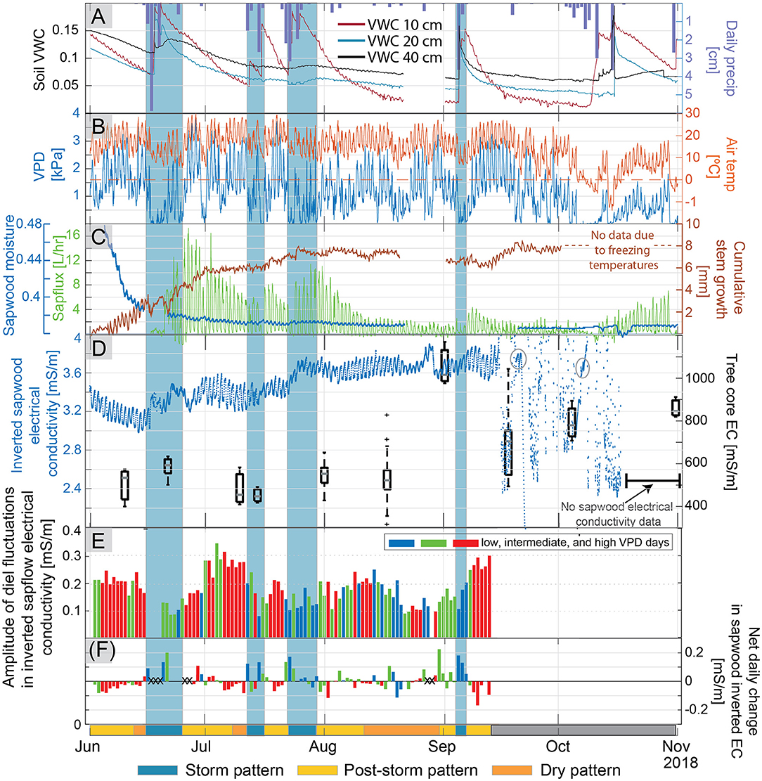
Figure 3. Trends through the growing season in (A) precipitation and soil volumetric water content at 20 and 40-cm depth in soil profile 2, (B) vapor pressure deficit (VPD) and air temperature measured 2 m above the ground surface, (C) sapwood moisture measured with the FDR sensor, sapflux, and cumulative stem growth measured via trunk diameter, and (D) temperature-corrected average inverted electrical conductivity (EC) in the tree with box plots of fluid EC measured in tree cores extracted from neighboring trees on the right axis. The variance in fluid EC increased later in the season relative to earlier season measurements. The two warm multi-day periods where an EC signal is again apparent and outlined with gray circles. (E) Amplitudes of diel fluctuations in inverted sapwood electrical conductivity. Colors signify the three bins used to distinguish between “low VPD” days (blue), “intermediate VPD” (green), and “high VPD” (red) days. Amplitudes in inverted sapwood electrical conductivity could not be determined past September 15 due to noise. (F) Net daily change in sapwood electrical conductivity (e.g., the difference between inverted sapwood electrical conductivity at sunrise between 2 consecutive days), colored by our low, intermediate, and high VPD classification. Large anomalous net daily changes are marked with Xs, these changes often corresponded with storm events and may result from changes in bark moisture. On the bottom x-axis, a single bar denotes three distinct patterns (storm, post-storm, and dry pattern) observed in the diel fluctuations of inverted sapwood electrical conductivity, described in detail in section Temporal Patterns in Inverted Sapwood Electrical Conductivity. Shaded blue regions across all subpanels correspond to storm.
Sapflux
Sapflux generally decreased from late June through mid-August, when it leveled off due to dry conditions (Figure 3C); however, following large storm events there were day-to-multi-day periods when sapflow increased. Diurnal fluctuations in sapflux were continuous over the course of the study period except during a stormy 4-day period starting on June 16 and a 6-day period starting on October 11 when VPD was ~0 and snow flurried (Figures 3B,C).
Sapwood Moisture and Diel Changes in Trunk Diameter
Sapwood moisture measured with the FDR sensor followed the same trend as soil moisture, suggesting that the observed seasonal depletion of sapwood moisture may have resulted from decreases in subsurface moisture availability (Figure 3C). Sapwood moisture decreased rapidly from early to late June, as high transpiration rates depleted soil moisture (Figures 3A,C). In late June, sapwood moisture stabilized, and then decreased slightly over the remainder of the study period; however, due to power loss, sapwood moisture was not monitored between August 21 and September 1.
Diel fluctuations in sapwood moisture were consistently observed between June and August 21 and followed the inverse pattern of transpiration. As noted earlier, peaks and troughs of diel fluctuations in sapwood moisture could not be determined exactly because small changes in moisture content that occurred within the 30-min measurement intervals were often below the measurement resolution (0.001 m3/m3) of the TEROS 12 soil moisture sensor (Supplementary Figure 1). When power was restored to the sensor on September 1, diel patterns were “box-shaped” and the only conclusion that could be drawn is that nighttime and morning moisture content is greater than afternoon and evening moisture content and that moisture levels continue to decrease until the September 5 storm event, which saturated soils. In contrast to our results, previous studies using FDR sensors in trees showed clear diel patterns in stem moisture (Holbrook et al., 1992; Hao et al., 2013; Matheny et al., 2017) where the timing of peaks and troughs could be easily distinguished. This may be due to the fact that these studies collected data at shorter time intervals (5–10 min vs. 30-min in our study) and/or because the magnitude of changes in moisture were greater, and incremental changes throughout the day were not as close to the resolution limits of the sensor.
Trunk growth increased substantially in June and gradually through July, and would often occur more rapidly following precipitation events (Figure 3C). When dendrometer measurements are made over the bark (as was done in this study), the measured change in stem diameter may be affected by absorption and evaporation of water from dead bark tissue (Mencuccini et al., 2017; Oberhuber et al., 2020). Rapid increases in stem diameter associated with storm events followed by a decline in stem diameter (e.g., July 15 and 25) likely result from bark water absorption and do not suggest growth occurred (Figure 3C). Consequently, diurnal patterns in stem water storage could not be thoroughly investigated with the dendrometer measurements; however, seasonal patterns dominated by irreversible radial stem growth could be distinguished. Tree diameter increased 7.6 mm between June 1 and October 1 according to the dendrometer; an 8.5 mm increase in tree diameter at breast height was measured manually with a DBH tape between May 27 and October 4, confirming that seasonal changes (i.e., irreversible radial stem growth) monitored with the dendrometer were reasonable.
Trunk Electrical Conductivity
Radial Patterns in Inverted Sapwood Electrical Conductivity
In the electrical conductivity images, there was a clear transition from high to low electrical conductivity at ~15-cm from the center of the tree, which matches the transition from sapwood to heartwood identified in the six tree cores at ~14-cm from the center of the tree (Figure 4A). Core measurements indicated that the sapwood/heartwood boundary was shallower on the north-facing, upslope side of the tree (at ~8.5 cm from the bark), and better match the potential heartwood/sapwood boundary apparent in the ERI images on this side (Figure 4A). ERI inversions from the tree trunk cross-section also revealed that the south-facing side of the trunk between electrodes 4 and 8 was generally more conductive than the north-facing side (Figure 4A), supporting the idea of thicker sapwood (and/or a more active xylem) on the south side. Al Hagrey (2006) observed that there is typically more sapflow activity on the sunlit side of the tree, so the higher electrical conductivity on the south-facing side of the ponderosa pine stem may suggest that more moisture is stored in this region to supply the increased sapflow activity.
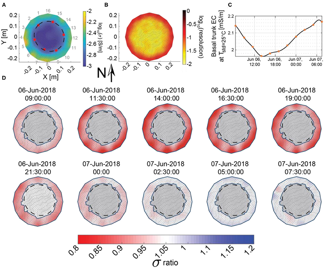
Figure 4. (A) Electrical conductivity distribution on June 6 (a clear warm day used as time zero for the ERI differencing) at 06:30 h, with electrode locations (1–16) around the outside and the location of heartwood/sapwood transition from tree cores (red squares) interpolated by a best-fit ellipse (black dashes). (B) Average diagonal of the resolution matrix for all 11 surveys between June 6 at 06:30 h and June 7 at 07:30 h, (C) spline interpolation (black line) of the median bulk apparent conductivity of the sapwood (orange squares) over a 25-h period, and (D) differences in inverted sapwood electrical conductivity with respect to the June 6 at 06:30 electrical conductivity model shown in (A). Gray regions were removed from our analysis because these areas corresponded to the heartwood, which is not expected to significantly contribute to daily water use and because the ERI resolution was poor.
The average resolution for ERI surveys was highest in the outermost 4.3 cm of the tree trunk and decreased toward the center of the trunk (Figure 4B) as would be expected (e.g., Oldenburg and Li, 1999). Daily changes in inverted electrical conductivity were also greatest in the outermost portions of sapwood (Figure 4D). While ERI has better resolution of changes in this area, this result is also consistent with the observations by Domec et al. (2005) in an old growth ponderosa pine, which indicated that outer sapwood contributed more than 57% to the total trunk water depletion, compared with 31 and 12% for the middle and inner sapwood.
Temporal Patterns in Inverted Sapwood Electrical Conductivity
The diel variations in inverted sapwood electrical conductivity (Figure 4) followed tree water storage patterns observed in other pine species using sapflow, FDR sensor, or dendrometer methods (e.g., Zweifel et al., 2001; Cermák et al., 2007; Verbeeck et al., 2007a; Matheny et al., 2015), where tree water storage decreased from sunrise to the early afternoon and increased in the afternoon and into the night (Figure 3D). Diel fluctuations in inverted sapwood electrical conductivity are evident throughout the summer, with the exception of the storm event in mid-June and after September 15 when there is considerable noise in the measurements (Figure 3D).
Variable meteorological and soil moisture conditions led to three distinct diel patterns in inverted sapwood electrical conductivity during the growing season (Figure 3):
• Storm pattern: During stormy periods (e.g., periods of low evaporative demand and high soil water content such as June 22–25; Figures 3A,C), inverted sapwood electrical conductivities mostly increased from one morning to the next (Figure 3F), with little to no decrease in inverted sapwood electrical conductivity during the daytime hours. Diel fluctuations were often not apparent or had a small amplitudes (Figures 3D,E).
• Post-storm pattern: After storm events, soils were relatively moist, evaporative demand was high, sapflow increased, and amplitudes of diel fluctuations in inverted sapwood electrical conductivity generally increased (e.g., June 28–July 10 and July 28–August 11; Figure 3). The largest amplitude diel fluctuations in inverted sapwood electrical conductivity were not observed on days with the greatest sapflow rates, which occurred ~3–4 days after the storm event when soils were moist (Figures 3C,E). Rather, amplitudes of diel fluctuations in inverted sapwood electrical conductivity were greatest when soil moisture neared pre-storm event levels, indicating a transition to a dry period. Appreciable decreases in inverted sapwood electrical conductivity from one morning to the next corresponded with large amplitude diel fluctuations in that dataset (Figures 3E,F).
• Dry pattern: During dry periods, soil moisture was low, evaporative demand was high, and amplitudes of diel fluctuations in inverted sapwood electrical conductivity decreased (e.g., August 14–September 29; Figure 3). There was generally a small decrease in inverted sapwood electrical conductivity from one morning to the next (Figure 3F), and no irreversible growth occurred under these conditions.
Starting in mid-September, diel fluctuations in inverted sapwood electrical conductivity could not be identified because noise increased drastically; at this time, average daily temperatures decreased, nighttime temperatures were close to freezing, soils were dry, daily transpiration was near a summertime low, and the dendrometer recorded a decrease in trunk diameter (Figure 3). The source(s) of noise are not clear; however, the changes in environmental conditions may have affected the coupling of electrodes used for the electrical conductivity measurements. The noise was nearly constant throughout the rest of the study period, except during two warm multi-day periods following the storm events on September 19 and the early-October snowstorm where a signal is once again apparent (Figure 3D).
We expected that as conditions became progressively drier through the growing season that we would see a reduction in inverted sapwood electrical conductivities because there would be less sapwood moisture. However, inverted sapwood electrical conductivity of the tree trunk generally increased from June 1 to September 15, with the largest increases in June and July (Figure 3D). This result was also observed and went largely unexplained in Mares et al. (2016). Fluid electrical conductivity extracted from nearby ponderosa pine trees over the course of the season was relatively constant from June through August (Figure 3D), so it seems unlikely that a change in fluid electrical conductivity is responsible for the seasonal increase in inverted sapwood electrical conductivity. The increased inverted sapwood electrical conductivity from June 1 to August 1 may be due to new growth. If we approximate the sapwood area as a ring with a radius of 10 cm (e.g., the average sapwood thickness, determined by the difference between measured inner and outer sapwood in the six cores), and assume that the additional 8 mm of growth was mostly sapwood, then between June 1 and September 15 the amount of sapwood increased by ~5%, which would increase the water storage capacity and subsequently the measured electrical conductivity. It is unclear if a 5% increase in outer portion of sapwood is substantial enough to significantly increase the hydraulic capacity of sapwood over the season, and this 5% would be even smaller if the conversion of sapwood to heartwood was considered. However, Domec et al. (2005) found that the outer sapwood of a ponderosa pine accounted for ~60% of the water stored in the sapwood, suggesting that new stem growth may hold considerably more water between its tissues.
Another factor considered was the influence of the fixed inversion grid used throughout the study period, which did not account for stem growth. According to Pouillet's law, , where ρ is electrical resistivity, l is the path length, R is resistance, and A is the cross-sectional area, increasing the cross-sectional area would lead to a decrease in the apparent resistivity, and thus reduce the resistance, ultimately increasing the electrical conductivity. To test the influence of an increase in cross-sectional area we inverted surveyed data from August 6 at 06:00 (when the dendrometer data suggest that seasonal growth had mostly stabilized) with a grid that was expanded radially by 8 mm. Results from the expanded grid could not be directly compared on an element-by-element basis because the fixed grid included an additional 116 triangular elements to account for the increased cross-sectional area. However, the expanded grid led to no visible change in the spatial distribution of electrical conductivity and the difference in the median electrical conductivity of the expanded grid was slightly greater (<1%) than the median electrical conductivity of the fixed grid, suggesting that the error introduced by the fixed grid does not account for the observed seasonal increase in sapwood electrical conductivity.
Diel Relations Between Data Sets
Between Sapflow and Trunk Electrical Conductivity
In an isohydric species such as ponderosa pine, we expect that when sapwood and soil moisture stores are limited, the likely physiological response to an increase in evaporative demand would be to limit sapflow by reducing stomatal conductance. This was supported in our data by: (1) trends in amplitudes of diurnal fluctuations in sapflow (detailed in section Temporal Patterns in Inverted Sapwood Electrical Conductivity), which progressively decreased as soil moisture and sapwood moisture decreased (Figures 3A,C); and (2) trend in peak times of diurnal fluctuations in sapflow, which peaked earlier in the day as conditions dried (Figure 5). In the latter part of post-storm patterns (e.g., ~4–5 days after the storm event), soil moisture neared pre-storm event levels and the magnitude of diurnal amplitudes in sapflow fluctuations decreased, but amplitudes in inverted sapwood electrical conductivity fluctuations increased (e.g., Figure 3E), suggesting the tree became increasingly reliant on sapwood moisture stores as soil moisture decreased. The relative importance of sapwood moisture at the transition period was also apparent in the XWT and WTC between sapflow and inverted electrical conductivity (Figures 6C,D). Lag times increased as soils dried and the longest lag times were observed in the latter part of post-storm patterns when soil neared pre-storm event levels, but sapwood moisture remained high (Figure 6E). The effects of high sapwood moisture were apparent when comparing days within the latter part of post-storm patterns to days in the dry period (Figure 7A). On days within the post-storm patterns (e.g., July 10, Figure 7A), inverted electrical conductivities decrease rapidly in the morning hours as sapwood moisture is used to sustain high rates of sapflow and in the late-morning/early-afternoon sapwood moisture is used as at a slower rate to help maintain sapflow rates. This extended period and high rate of sapwood moisture use subsequently increases the time it takes to replenish sapwood moisture stores in the late afternoon and evening hours, and ultimately increases lag times between sapflow and inverted sapwood electrical conductivity. On days within the dry period (e.g., August 23, Figure 7A), smaller amplitude diel fluctuations in inverted electrical conductivity suggest that only small amounts of internal water storage water were released to supply transpiration in the early morning before sapflow rapidly decreased in response to increased evaporative demand. This had the effect of reducing time lags between sapflow and sapwood inverted electrical conductivities (Figure 6E). These observations are in agreement with other studies, which found that tree species with high sapwood water-storage capacity (i.e., ponderosa pines) have a longer period to react physiologically to an increase in evaporative demand (Martins et al., 2016); however, as shown in the hysteresis method employed by Matheny et al. (2014), this response window is shortened as sapwood moisture is depleted during prolonged drought.
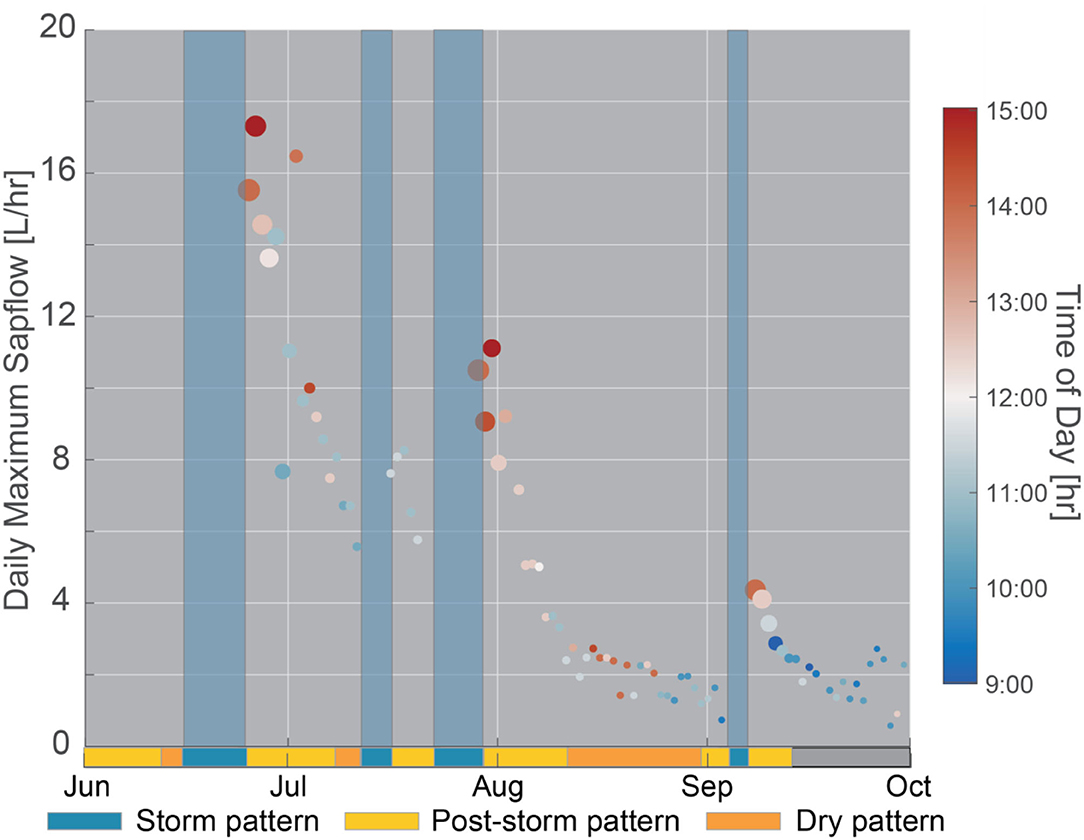
Figure 5. Daily maximum sapflow through time. Points within storm events were removed because the time of maximum sapflow was controlled by the timing of the storm event. Dot size indicates soil moisture and dot color denotes the time of peak sapflow. Shaded blue regions across all subpanels correspond to storm patterns. On the bottom x-axis, a single bar denotes three distinct patterns (storm, post-storm, and dry pattern) observed in the diel fluctuations of inverted sapwood electrical conductivity, described in detail in section Temporal Patterns in Inverted Sapwood Electrical Conductivity. The gray bar corresponds with the period when patterns could not be distinguished due to noise in inverted sapwood electrical conductivity data.
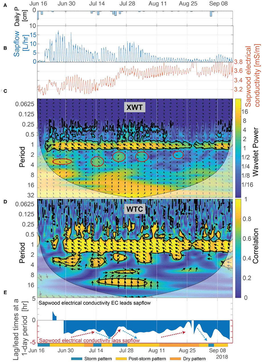
Figure 6. (A) Daily precipitation, (B) sapflow and inverted sapwood electrical conductivity, (C) the XWT of sapflow and inverted sapwood electrical conductivity, (D) the WTC of sapflow and inverted sapwood electrical conductivity, and (E) the lead/lag calculated using Equation (7) and the phase angle of arrows at a 1-day period between sapflow and inverted sapwood electrical conductivity. Regions in time-frequency space in the XWT that had moderately high wavelet power, periods >1-day, and where the WTC identified high correlation are outlined with red circles. The regions outlined in red coincide with the storm events. Red arrows highlight periods when we hypothesize that progressively drier conditions increased stomatal regulation, and subsequently decreased lag times. Blue arrows highlight periods when we hypothesize that increased moisture, due to precipitation, decreased stomatal regulation, subsequently increasing lag times.
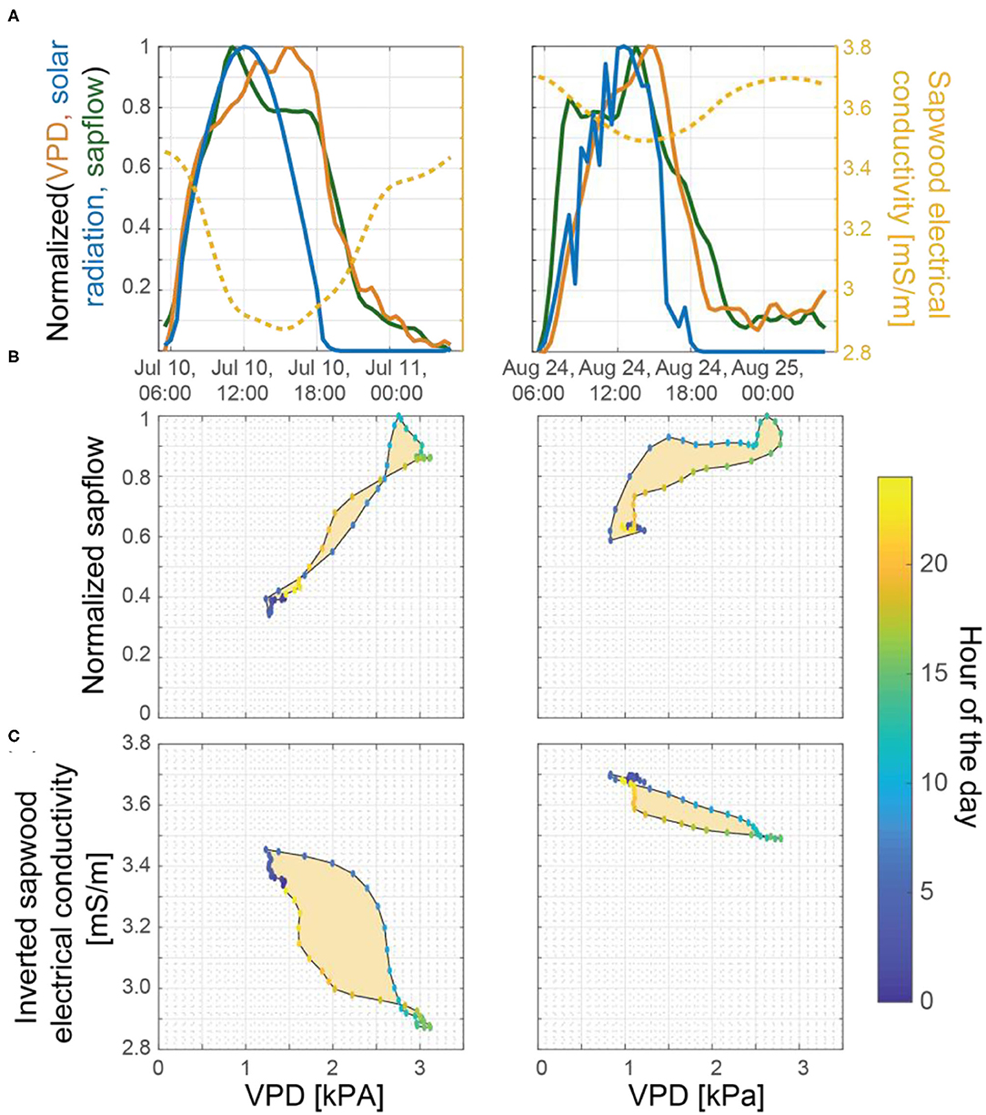
Figure 7. (A) Normalized VPD (orange line), solar radiation (blue line), and sapflow (green) with inverted sapwood electrical conductivity (yellow line) on July 10 and August 24, 2018. These 2 days were selected for comparison because both days were considered to be mostly sunny, high VPD days, that occurred at the tail end of multi-day dry periods, but also because soil moisture availability was limited by August 24 and not on July 10 (Figure 3A), providing a contrast. Hysteresis between VPD and (B) sapflow and (C) inverted sapwood electrical conductivity.
To further evaluate the relations among sapflow, inverted sapwood electrical conductivity, and evaporative demand established in the wavelet analysis, we also employed hysteresis method. The degree of hysteresis between VPD and inverted sapwood electrical conductivity, which is created by the time lag between them, generally decreased with increasing drought severity (e.g., July 10 vs. August 24; Figure 7). This finding supported our interpretation that lower sapwood moisture and soil moisture led to a more rapid stomatal response. Diel tree water storage patterns are likely more evident in the degree of hysteresis between VPD and inverted sapwood electrical conductivity than with sapflow because inverted sapwood electrical conductivity is sensitive to changes in sapwood moisture, while sapflow cannot be directly tied to changes in sapwood moisture (i.e., Figure 7B vs. Figure 7C). However, there were many days throughout the growing season when the relation between VPD and sapflow or inverted sapwood electrical conductivity did not form a simple hysteretic loop, and thus the role of tree water storage could not be evaluated. These results highlight the strength of the wavelet analysis method, which can continuously quantify diel relations between transpiration and inverted sapwood electrical conductivity through time.
Meteorological Controls on Diel Changes in Sapwood Moisture
Results from our wavelet analysis suggest that the influence of solar radiation on inverted sapwood electrical conductivity is mostly constant throughout the summer, with the exception of stormy periods (Figures 8C,D). Statistically significant wavelet power is observed at a 1-day period in the XWT transform from June 1 to September 15, with the exception of periods that overlap with large storm events (Figure 8C). Nearly-constant phase arrows and high correlation observed in the WTC over the same time period indicate that solar radiation and inverted sapwood electrical conductivity are out of phase and that there likely is a causal relation between them, with inverted sapwood electrical conductivity lagging solar radiation by an average of ~4.3 h (Figures 8D,E). During storm events, phase arrows at a 1-day period increased to ~5 h lag in the XWT, correlation decreased in the CWT, and wavelet power decreased in the XWT, indicating a weak or non-existent relation between incoming solar radiation and inverted sapwood electrical conductivity due to cloud cover and limited transpiration (Figures 3B,D; Figures 8A,C). The influence of solar radiation alone cannot fully explain the variability that drives the three patterns outlined in section Temporal Patterns in Inverted Sapwood Electrical Conductivity due to minimal variability in lag times between solar radiation and inverted sapwood electrical conductivity over the summer.
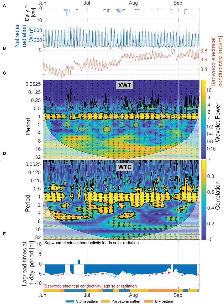
Figure 8. (A) Daily precipitation, (B) net solar radiation and inverted sapwood electrical conductivity, (C) the XWT of solar radiation and inverted sapwood electrical conductivity, (D) the WTC of solar radiation and inverted sapwood electrical conductivity, and (E) the lead/lag time at a 1-day period between solar radiation and inverted sapwood electrical conductivity. Regions in time-frequency space in the XWT that had moderately high wavelet power, periods >1-day, and where the WTC identified high correlation are outlined with red circles in (C). The regions outlined in red coincide with the storm events. Red arrows in (E) highlight dry conditions that increased stomatal regulation, and subsequently decreased lag times. Blue arrows in (E) highlight periods of increased moisture, due to precipitation, which decreased stomatal regulation, subsequently increasing lag times.
Patterns identified in the wavelet analysis between VPD and inverted sapwood electrical conductivity correspond to the three patterns noted earlier in the inverted sapwood electrical conductivity. From June 1 to September 15, there was considerably more variability in the XWT and WTC of VPD and inverted sapwood electrical conductivity at the 1-day period when compared to the XWT and WTC of solar radiation and inverted sapwood electrical conductivity (Figures 8C,D vs. Figures 9C,D); this result suggests that changes in VPD drive most of the observed variability in daily reductions of sapwood moisture. A relation between VPD and inverted sapwood electrical conductivity is not present during the storm pattern (e.g., June 15–28) or is weakened during smaller storm events (e.g., storm events in mid-July; Figure 9D). As conditions dry post-storm, lags between inverted sapwood electrical conductivity and VPD decreased while correlation between the two increased, suggesting increased evaporative demand led to stronger coupling between VPD and sapwood moisture use (Figures 9D,E). The exception to this trend was the post-storm period from July 30 to August 19, where lag times between inverted sapwood electrical conductivity and VPD were mostly constant and correlations were high, suggesting that the ponderosa pine may have employed an increasingly conservative water strategy as moisture availability decreased and evaporative demand increased. In the dry pattern (e.g., August 19–27), lag times between VPD and inverted sapwood electrical conductivity decrease to nearly a zero lag (Figure 9E). The relatively rapid decrease in lag times during this period corresponds with decreasing amplitudes in inverted sapwood electrical conductivity and the lowest observed sapflow rates outside of stormy periods when VPD was zero. These observations suggest that sapwood hydraulic capacity and soil moisture stores could only sustain small amounts of transpiration after extended drought (July 28–Septmebr 29) without a large storm event. Ultimately, both solar radiation and VPD are important controls on diel changes in inverted sapwood electrical conductivity; however, variability in daily reductions of sapwood moisture could not be fully explained without the effects of VPD.
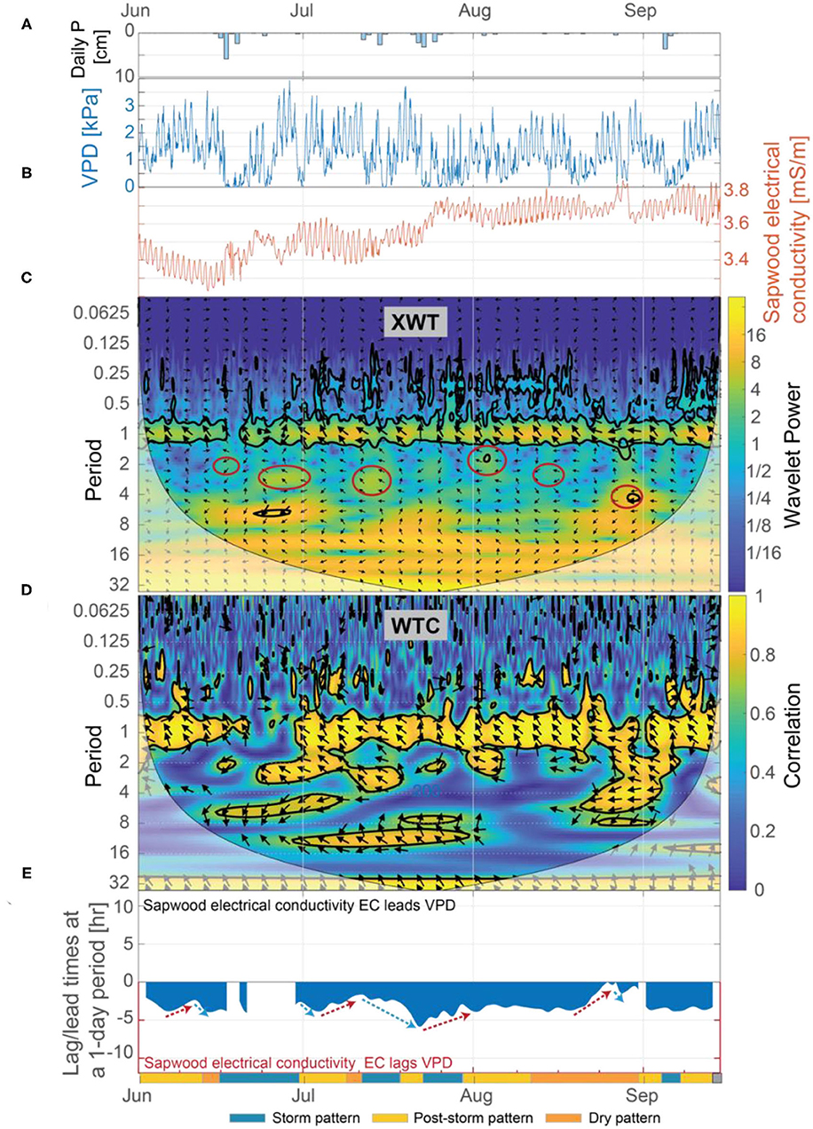
Figure 9. (A) Daily precipitation, (B) vapor pressure deficit (VPD) and inverted sapwood conductivity, (C) the XWT of VPD and inverted sapwood electrical conductivity, (D) the WTC of VPD and inverted sapwood electrical conductivity, and (E) the lag time between VPD and inverted sapwood electrical conductivity. Regions in time-frequency space in the XWT that had moderately high wavelet power, had periods >1-day, and where the WTC identified high correlation are outlined with red circles. The regions outlined with red circles coincide with the storm events. Red arrows in (E) highlight periods when we hypothesize that progressively dryer conditions increased stomatal regulation, and subsequently decreased lag times. Blue arrows in (E) highlight periods when we hypothesize that increased moisture, due to precipitation, decreased stomatal regulation, and subsequently increasing lag times.
Between Soil Moisture and Trunk Electrical Conductivity
The inverse relation between inverted sapwood electrical conductivity and soil moisture is strong only when soils are dry. The XWT and WTC indicate that during dry periods there is an inverse relation between soil moisture and inverted sapwood electrical conductivity; phase arrows suggest that soil moisture at 20-cm depth and inverted sapwood electrical conductivity were in phase, with inverted sapwood electrical conductivity lagging soil moisture at a 1-day period (Figures 10C,D). Lag times between soil moisture and inverted sapwood electrical conductivity increased from a nearly zero lag in early July to a 5-h lag by mid-July (Figure 10E). In subsequent dry periods, lag times remain relatively constant at ~5 h. The longer lag times may be caused by limits of root water uptake in drying soils. Correlation between inverted sapwood electrical conductivity and soil moisture increased as lags increase during dry periods (Figures 10D,E), suggesting that link between soil moisture and internal water strengthens during prolonged drought. One may expect that as soils dry, the ability to replenish internal water stores would decrease, subsequently weakening the connection between soil moisture and internal water storage. However, ponderosa pine are known to use a deep rooting strategy, which enables redistribution of deeper water stores to shallow soils (e.g., Brooks et al., 2002). Mares et al. (2016) suggested hydraulic redistribution to explain ERI data in a ponderosa pine located <60 m from our study tree. Given the strong inverse relation between soil moisture and inverted sapwood electrical conductivity identified during dry periods, we assume that the ponderosa pine is actively relying on deeper water sources.
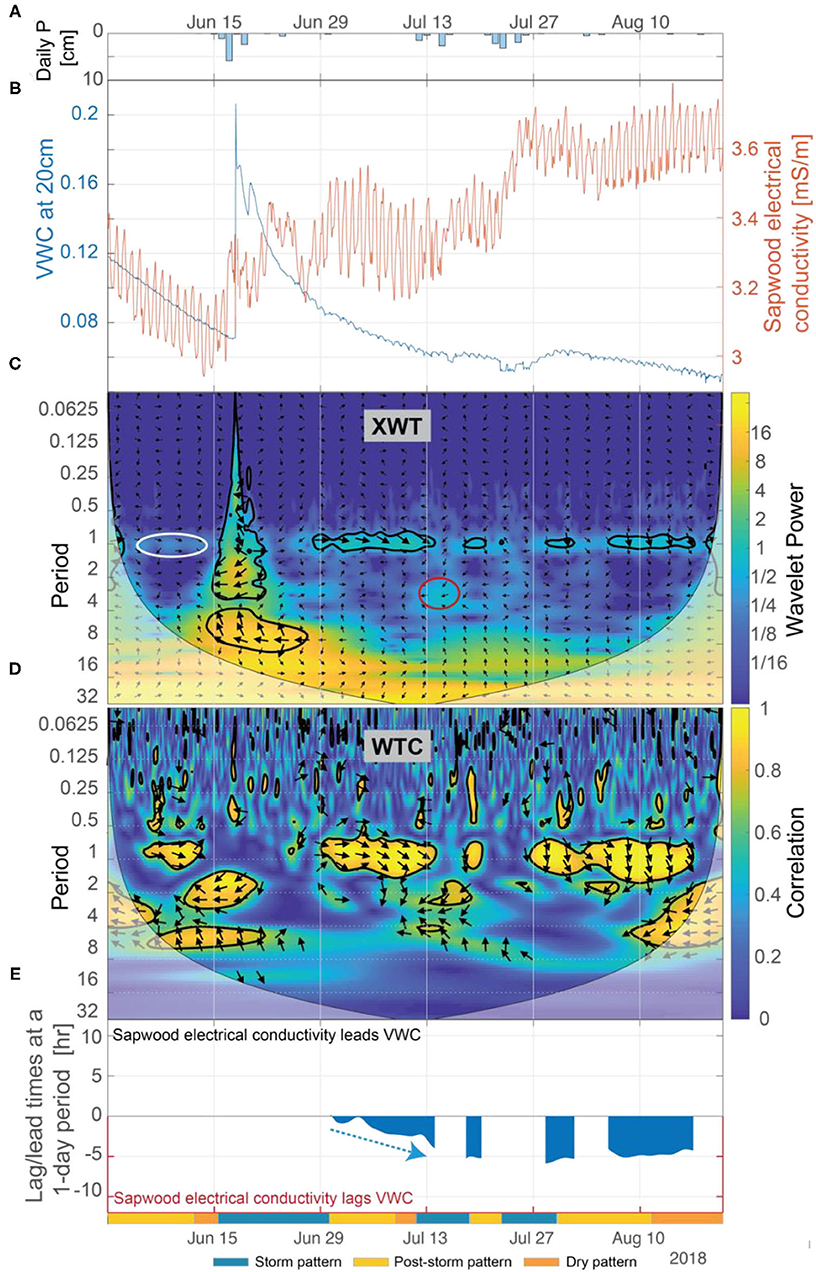
Figure 10. (A) Daily precipitation, (B) soil VWC at 20-cm depth and inverted sapwood electrical conductivity, (C) the XWT of soil VWC and inverted sapwood electrical conductivity, (D) the WTC of soil VWC and inverted sapwood electrical conductivity, and (E) the lead/lag time at a 1-day period between soil VWC and inverted sapwood electrical conductivity. Regions in time-frequency space in the XWT that: were not already identified as significant (black contour lines), had moderately high wavelet power, had periods >1-day, and where the WTC identified high correlation are outlined with red circles. The white ellipse at ~1-day period highlights a period when the WTC suggests that a 13-day time period of increasing inverted sapwood electrical conductivity between July 14 and July 27 may cause the subsequent (delayed by 6 days as indicated by phase arrows) 12-day period of decreased sapflow occurring between August 2 and 14. Red arrows highlight periods when we hypothesize that progressively dryer conditions increased stomatal regulation, and subsequently decreased lag times. Blue arrows highlight periods when we hypothesize that increased moisture, due to precipitation, decreased stomatal regulation, and subsequently increasing lag times.
The Influence of Environmental Changes at Periods Longer Than 1-day on Inverted Sapwood Electrical Conductivity
The XWT and WTC indicate that there are regions in time-frequency space at periods >1 day with high wavelet power and significant correlation between the driving environmental variables (solar radiation, VPD, soil moisture, and sapflow) and inverted sapwood electrical conductivities (Figures 6, 8–10). These significant regions occur mostly within 2–4 day periods and correspond with storm events. Nearly all phase arrows within these regions are out of phase, which indicates that inverted sapwood electrical conductivities increased and the environmental variables decreased. The XWTs and WTCs identified some regions at periods longer than 2–4 days that were significant. However, from a physical process standpoint, it is not clear how these regions relate to sapwood moisture patterns; thus, interpretations of these regions are not discussed here.
Conclusions
Together, time-lapse ERI and wavelet analysis provided insight at the relevant spatial and temporal scales needed to evaluate relations between tree water storage and daily transpiration. Wavelet analyses successfully deconstructed complicated time series data into periodic (e.g., 24-h) and non-periodic events, which enabled us to evaluate the effects of extended dry periods and storm events on tree water storage. Diel patterns in inverted sapwood electrical conductivity followed a pattern similar to tree water storage patterns measured in other tree species using different methods (e.g., FDR sensors, Matheny et al., 2015, 2017) and followed diel patterns measured in our embedded FDR sensor, suggesting that inverted sapwood electrical conductivity was effective at monitoring changes in tree water storage. Seasonal increases in inverted sapwood electrical conductivity did not result from an increase in xylem fluid electrical conductivity. Instead, increases in inverted sapwood electrical conductivity may result from new growth, which primarily occurred in June and after large storm events. Physical relations between tree water storage as estimated by ERI and sapflow, solar radiation, VPD, and soil moisture were investigated and our key findings were:
• Diel amplitudes of inverted sapwood electrical conductivity indicated that tree water storage use was greatest ~4–5 days after storm events, when sapwood hydraulic capacity was high and storm event water was gone. Tree water storage continued to be relied upon during dry periods, but as drought conditions progressed tree water storage capacity to contribute to transpiration decreased (e.g., amplitudes in inverted sapwood electrical conductivity decreased).
• Wavelet analyses revealed that short time lags between sapflow and inverted sapwood electrical conductivity correspond with dry conditions, when stomatal conductance is lowered to avoid dehydration. Longer lags between sapflow and inverted sapwood electrical conductivity were observed when conditions were relatively wet. Increased soil moisture and sapwood moisture during these wet periods enabled higher rates of sapflow and increased the time that the ponderosa pine could safely transpire, subsequently increasing the amount of tree water storage used and the time tree water storage was relied upon to supply transpiration.
• The diel variability in sapwood moisture could not be fully explained without incorporating the effects of VPD.
The trends identified in tree water storage using ERI and wavelet analysis highlight how ponderosa pines respond to conditions on dry, south-facing hillslopes in Colorado montane forests Tree water storage was a vital resource that the ponderosa pine relied upon during intermittent dry periods typical of monsoon season in the Colorado Front Range. Our findings highlight (1) the utility of time-lapse ERI to provide insight into tree hydraulic function at spatial and temporal scales that cannot feasibly be achieved using traditional methods, and (2) the utility of wavelet analysis to efficiently extract information from ERI time series.
Data Availability Statement
The original contributions presented in the study are included in the article/Supplementary Material, further inquiries can be directed to the corresponding author.
Author Contributions
HB helped with data acquisition (e.g., sapflow), aided in the interpretation of the data, and provided a critical revision of the work. FD-L provided his expertise in time-series analysis, contributed to the wavelet analysis work, which was critical in untangling the complicated temporal signals, and also provided a critical review of the work. DM developed the inversion code in COMSOL, helped RH work through the inversions of the stem electrical conductivity data, and also helped analyses the electrical resistivity data and provided a critical review of our findings. KS made substantial contributions to the conception of the work, the analysis of the work, and was heavily involved in the drafting and critical review. All authors contributed to the article and approved the submitted version.
Funding
This work was supported by the National Science Foundation (EAR1446161, EAR1446231, EAR0724960, EAR2012730, and EAR2012669).
Author Disclaimer
Any use of trade, firm, or product names is for descriptive purposes only and does not imply endorsement by the U.S. Government.
Conflict of Interest
The authors declare that the research was conducted in the absence of any commercial or financial relationships that could be construed as a potential conflict of interest.
Publisher's Note
All claims expressed in this article are solely those of the authors and do not necessarily represent those of their affiliated organizations, or those of the publisher, the editors and the reviewers. Any product that may be evaluated in this article, or claim that may be made by its manufacturer, is not guaranteed or endorsed by the publisher.
Acknowledgments
We would like to thank Jackie Randell and Aaron Engers for their efforts in the field and assistance with in-lab analyses. Also, we thank Toby Minear for LiDAR data collection and processing.
Supplementary Material
The Supplementary Material for this article can be found online at: https://www.frontiersin.org/articles/10.3389/frwa.2021.682285/full#supplementary-material
Data have been submitted to CUAHSI's HydroShare (http://www.hydroshare.org/resource/6e102de63a7943e1900aa8c6a8d412ac), and will be released upon publication.
References
Addison, P. S. (2018). Introduction to redundancy rules: the continuous wavelet transform comes of age. Philos. Trans. R. Soc. A Math. Phys. Eng. Sci. 376:258. doi: 10.1098/rsta.2017.0258
Al Hagrey, S. A. (2006). Electrical resistivity imaging of tree trunks. Near Surf. Geophys. 4, 179–187. doi: 10.3997/1873-0604.2005043
Al Hagrey, S. A. (2007). Geophysical imaging of root-zone, trunk, and moisture heterogeneity. J. Exp. Bot. 58, 839–854. doi: 10.1093/jxb/erl237
Arora, B., Dwivedi, D., Hubbard, S. S., Steefel, C. I., and Williams, K. H. (2016). Identifying geochemical hot moments and their controls on a contaminated river floodplain system using wavelet and entropy approaches. Environ. Model. Softw. 85, 27–41. doi: 10.1016/j.envsoft.2016.08.005
Befus, K. M., Sheehan, A. F., Leopold, M., Anderson, S. P., and Anderson, R. S. (2011). Seismic constraints on critical zone architecture, Boulder Creek Watershed, Front Range, Colorado. Vadose Zo. J. 10, 915–927. doi: 10.2136/vzj2010.0108
Benson, A. R., Koeser, A. K., and Morgenroth, J. (2019). Estimating conductive sapwood area in diffuse and ring porous trees with electronic resistance tomography. Tree Physiol. 39, 484–494. doi: 10.1093/treephys/tpy092
Bieker, D., and Rust, S. (2010). Non-destructive estimation of sapwood and heartwood width in scots pine (Pinus sylvestris L.). Silva Fenn. 44, 267–273. doi: 10.14214/sf.153
Bohrer, G., Mourad, H., Laursen, T. A., Drewry, D., Avissar, R., Poggi, D., et al. (2005). Finite element tree crown hydrodynamics model (FETCH) using porous media flow within branching elements: a new representation of tree hydrodynamics. Water Resour. Res. 41, 1–17. doi: 10.1029/2005WR004181
Borchert, R. (1994). Soil and stem water storage determine phenology and distribution of tropical dry forest trees. Ecology 75, 1437–1449. doi: 10.2307/1937467
Brooks, J. R., Meinzer, F. C., Coulombe, R., and Gregg, J. (2002). Hydraulic redistribution of soil water during summer drought in two contrasting Pacific Northwest coniferous forests. Tree Physiol. 22, 1107–1117. doi: 10.1093/treephys/22.15-16.1107
Bunce, J. A. (2006). How do leaf hydraulics limit stomatal conductance at high water vapour pressure deficits? Plant Cell Environ. 29, 1644–1650. doi: 10.1111/j.1365-3040.2006.01541.x
Burgess, S. S. O., Adams, M. A., Turner, N. C., Beverly, C. R., Ong, C. K., Khan, A. A. H., et al. (2001). An improved heat pulse method to measure low and reverse rates of sap flow in woody plants. Tree Physiol. 21, 589–598. doi: 10.1093/treephys/21.9.589
Burgess, S. S. O., and Dawson, T. E. (2008). Using branch and basal trunk sap flow measurements to estimate whole-plant water capacitance: a caution. Plant Soil 305, 5–13. doi: 10.1007/s11104-007-9378-2
Carrière, S. D., Ruffault, J., Pimont, F., Doussan, C., Simioni, G., Chalikakis, K., et al. (2020). Impact of local soil and subsoil conditions on inter-individual variations in tree responses to drought: insights from Electrical Resistivity Tomography. Sci. Total Environ. 698:134247. doi: 10.1016/j.scitotenv.2019.134247
Cermák, J., Kučera, J., Bauerle, W. L., Phillips, N., and Hinckley, T. M. (2007). Tree water storage and its diurnal dynamics related to sap flow and changes in stem volume in old-growth Douglas-fir trees. Tree Physiol. 27, 181–198. doi: 10.1093/treephys/27.2.181
Cobos, D., and Campbell, C. (2007). Correcting temperature sensitivity of ECH2O soil moisture sensors. Appl. Note. 13302–13394. Available online at: www.decagon.com
Cocozza, C., Marino, G., Giovannelli, A., Cantini, C., Centritto, M., and Tognetti, R. (2015). Simultaneous measurements of stem radius variation and sap flux density reveal synchronisation of water storage and transpiration dynamics in olive trees. Ecohydrology 8, 33–45. doi: 10.1002/eco.1483
Cowie, R. M., Knowles, J. F., Dailey, K. R., Williams, M. W., Mills, T. J., and Molotch, N. P. (2017). Sources of streamflow along a headwater catchment elevational gradient. J. Hydrol. 549, 163–178. doi: 10.1016/j.jhydrol.2017.03.044
Day-Lewis, F. D., Singha, K., and Binley, A. M. (2005). Applying petrophysical models to radar travel time and electrical resistivity tomograms: resolution-dependent limitations. J. Geophys. Res. Solid Earth 110, 1–17. doi: 10.1029/2004JB003569
Dey, A., and Morrison, H. F. (1979). Resistivity modeling for arbitrarily shaped three-dimensional structures. Geophysics 44, 753–780. doi: 10.1190/1.1440975
Domec, J. C., Pruyn, M. L., and Gartner, B. L. (2005). Axial and radial profiles in conductivities, water storage and native embolism in trunks of young and old-growth ponderosa pine trees. Plant Cell Environ. 28, 1103–1113. doi: 10.1111/j.1365-3040.2005.01347.x
Ewers, B. E., Gower, S. T., Bond-Lamberty, B., and Wang, C. K. (2005). Effects of stand age and tree species on canopy transpiration and average stomatal conductance of boreal forests. Plant Cell Environ. 28, 660–678. doi: 10.1111/j.1365-3040.2005.01312.x
Feddes, R. A., Hoff, H., Bruen, M., Dawson, T., De Rosnay, P., Dirmeyer, P., et al. (2001). Modeling root water uptake in hydrological and climate models. Bull. Am. Meteorol. Soc. 82, 2797–2809. doi: 10.1175/1520-0477(2001)082<2797:MRWUIH>2.3.CO;2
Ganthaler, A., Sailer, J., Bär, A., Losso, A., and Mayr, S. (2019). Noninvasive Analysis of tree stems by electrical resistivity tomography: unraveling the effects of temperature, water status, and electrode installation. Front. Plant Sci. 10:1455. doi: 10.3389/fpls.2019.01455
Garré, S., Coteur, I., Wongleecharoen, C., Kongkaew, T., Diels, J., and Vanderborght, J. (2013). Noninvasive monitoring of soil water dynamics in mixed cropping systems: a case study in Ratchaburi Province, Thailand. Vadose Zo. J. 12:129. doi: 10.2136/vzj2012.0129
Goldstein, G., Andrade, J. L., Meinzer, F. C., Holbrook, N. M., Cavelier, J., Jackson, P., et al. (1998). Stem water storage and diurnal patterns of water use in tropical forest canopy trees. Plant Cell Environ. 21, 397–406. doi: 10.1046/j.1365-3040.1998.00273.x
Grinsted, A., Moore, J. C., and Jevrejeva, S. (2004). Application of the cross wavelet transform and wavelet coherence to geophysical time series. Nonlinear Process. Geophys. 11, 561–566. doi: 10.5194/npg-11-561-2004
Guyot, A., Ostergaard, K. T., Lenkopane, M., Fan, J., and Lockington, D. A. (2013). Using electrical resistivity tomography to differentiate sapwood from heartwood: application to conifers. Tree Physiol. 33, 187–194. doi: 10.1093/treephys/tps128
Habberjam, G. M. (1967). On the application of the reciprocity theorem in resistivity prospecting. Geophysics 32, 918–919. doi: 10.1190/1.1439900
Hao, G. Y., James, K. W., Holbrook, N. M., and Guillermo, G. (2013). Investigating xylem embolism formation, refilling and water storage in tree trunks using frequency domain reflectometry. J. Exp. Bot. 64, 2321–2332. doi: 10.1093/jxb/ert090
Hartzell, S., Bartlett, M. S., and Porporato, A. (2017). The role of plant water storage and hydraulic strategies in relation to soil moisture availability. Plant Soil 419, 503–521. doi: 10.1007/s11104-017-3341-7
Hayley, K., Bentley, L. R., and Pidlisecky, A. (2010). Compensating for temperature variations in time-lapse electrical resistivity difference imaging. Geophysics 75:WA51. doi: 10.1190/1.3478208
Henderson, R. D., Day-Lewis, F. D., and Harvey, C. F. (2009). Investigation of aquifer-estuary interaction using wavelet analysis of fiber-optic temperature data. Geophys. Res. Lett. 36, 1–6. doi: 10.1029/2008GL036926
Holbrook, N. M. (1995). “Stem water storage,” in Plant Stems, ed B. L. Gartner (San Diego, CA: Academic Press), 151–174. doi: 10.1016/B978-012276460-8/50009-6
Holbrook, N. M., Burns, M. J., and Sinclair, T. R. (1992). Frequency and time-domain dielectric measurements of stem water content in the arborescent palm, Sabal palmetto. J. Exp. Bot. 43, 111–119. doi: 10.1093/jxb/43.1.111
Hong, L., Guo, J., Liu, Z., Wang, Y., Ma, J., Wang, X., et al. (2019). Time-lag effect between sap flow and environmental factors of Larix principis-rupprechtii Mayr. Forests 10:971. doi: 10.3390/f10110971
Huang, C. W., Domec, J. C., Ward, E. J., Duman, T., Manoli, G., Parolari, A. J., et al. (2017). The effect of plant water storage on water fluxes within the coupled soil–plant system. New Phytol. 213, 1093–1106. doi: 10.1111/nph.14273
Jarvis, M. E., James, G. B., and Landsberg, J. J. (1976). “Coniferous forest,” in Vegetation and the Atmosphere, Vol. 2, Case Studies, ed J. L. Montieth (London: Academic Press), 171–240.
Jarvis, P. G., and Mcnaughton, K. G. (1986). Stomatal control of transpiration: scaling up from leaf to region. Adv. Ecol. Res. 15, 1–49. doi: 10.1016/S0065-2504(08)60119-1
Kaner, A., Preisler, Y., Grünzweig, J., and Mau, Y. (2020). Internal water storage buffering maintains plant function under drought as described by a general hydraulic model. bioRxiv. doi: 10.1101/2020.02.11.943563
Kessouri, P., Furman, A., Huisman, J. A., Martin, T., Mellage, A., Ntarlagiannis, D., et al. (2019). Induced polarization applied to biogeophysics: recent advances and future prospects. Near Surf. Geophys. 17, 595–621. doi: 10.1002/nsg.12072
Köcher, P., Horna, V., and Leuschner, C. (2013). Stem water storage in five coexisting temperate broad-leaved tree species: significance, temporal dynamics and dependence on tree functional traits. Tree Physiol. 33, 817–832. doi: 10.1093/treephys/tpt055
Kumar, P., and Foufoula-Georgiou, E. (1997). Wavelet analysis for geophysical applications. Rev. Geophys. 35, 385–412. doi: 10.1029/97RG00427
Landsberg, J. J., Blanchard, T. W., and Warrit, B. (1976). Studies on the movement of water through apple trees. J. Exp. Bot. 27, 579–596. doi: 10.1093/jxb/27.4.579
Lin, C. J., Chung, C. H., Yang, T. H., and Lin, F. C. (2012). Detection of electric resistivity tomography and evaluation of the sapwood-heartwood demarcation in three Asia gymnosperm species. Silva Fenn. 46, 415–424. doi: 10.14214/sf.440
Lo Gullo, M. A., and Salleo, S. (1992). Water storage in the wood and xylem cavitation in 1-year-old twigs of Populus deltoides Bartr. Plant Cell Environ. 15, 431–438. doi: 10.1111/j.1365-3040.1992.tb00993.x
Loustau, D., Berbigier, P., Roumagnac, P., Arruda-Pacheco, C., David, J. S., Ferreira, M. I., et al. (1996). Transpiration of a 64-year-old maritime pine stand in Portugal. 1. Seasonal course of water flux through maritime pine. Oecologia 107, 33–42. doi: 10.1007/BF00582232
Luo, Z., Deng, Z., Singha, K., Zhang, X., Liu, N., Zhou, Y., et al. (2020). Temporal and spatial variation in water content within living tree stems determined by electrical resistivity tomography. Agric. For. Meteorol. 291:108058. doi: 10.1016/j.agrformet.2020.108058
Luo, Z., Guan, H., and Zhang, X. (2019). The temperature effect and correction models for using electrical resistivity to estimate wood moisture variations. J. Hydrol. 578:124022. doi: 10.1016/j.jhydrol.2019.124022
Maraun, D., and Kurths, J. (2004). Cross wavelet analysis: significance testing and pitfalls. Nonlinear Process. Geophys. 11, 505–514. doi: 10.5194/npg-11-505-2004
Mares, R., Barnard, H. R., Mao, D., Revil, A., and Singha, K. (2016). Examining diel patterns of soil and xylem moisture using electrical resistivity imaging. J. Hydrol. 536, 327–338. doi: 10.1016/j.jhydrol.2016.03.003
Martin, T. (2012). Complex resistivity measurements on oak. Eur. J. Wood Wood Prod. 70, 45–53. doi: 10.1007/s00107-010-0493-z
Martin, T., Nordsiek, S., and Weller, A. (2015). Low-Frequency Impedance Spectroscopy of Wood. J. Res. Spectrosc. 1, 1–9. doi: 10.5171/2015.910447
Martins, S. C. V., Mcadam, S. A. M., Deans, R. M., Damatta, F. M., and Brodribb, T. J. (2016). Stomatal dynamics are limited by leaf hydraulics in ferns and conifers: results from simultaneous measurements of liquid and vapour fluxes in leaves. Plant Cell Environ. 39, 694–705. doi: 10.1111/pce.12668
Matheny, A. M., Bohrer, G., Garrity, S. R., Morin, T. H., Howard, C. J., and Vogel, C. S. (2015). Observations of stem water storage in trees of opposing hydraulic strategies. Ecosphere 6, 1–13. doi: 10.1890/ES15-00170.1
Matheny, A. M., Bohrer, G., Vogel, C. S., Morin, T. H., He, L., Frasson, R. P. D. M., et al. (2014). Species-specific transpiration responses to intermediate disturbance in a northern hardwood forest. J. Geophys. Res. Biogeosciences 119, 2292–2311. doi: 10.1002/2014JG002804
Matheny, A. M., Garrity, S. R., and Bohrer, G. (2017). The calibration and use of capacitance sensors to monitor stem water content in trees. J. Vis. Exp. 2017:57062. doi: 10.3791/57062
McCulloh, K. A., Domec, J. C., Johnson, D. M., Smith, D. D., and Meinzer, F. C. (2019). A dynamic yet vulnerable pipeline: integration and coordination of hydraulic traits across whole plants. Plant Cell Environ. 42, 2789–2807. doi: 10.1111/pce.13607
Meinzer, F. C. (1993). Stomatal control of transpiration. Trends Ecol. Evol. 8, 289–294. doi: 10.1016/0169-5347(93)90257-P
Meinzer, F. C., Brooks, J. R., Domec, J. C., Gartner, B. L., Warren, J. M., Woodruff, D. R., et al. (2006). Dynamics of water transport and storage in conifers studied with deuterium and heat tracing techniques. Plant, Cell Environ. 29, 105–114. doi: 10.1111/j.1365-3040.2005.01404.x
Mencuccini, M., Salmon, Y., Mitchell, P., Hölttä, T., Choat, B., Meir, P., et al. (2017). An empirical method that separates irreversible stem radial growth from bark water content changes in trees: theory and case studies. Plant Cell Environ. 40, 290–303. doi: 10.1111/pce.12863
Mirfenderesgi, G., Bohrer, G., Matheny, A. M., Fatichi, S., de Moraes Frasson, R. P., and Schäfer, K. V. R. (2016). Tree level hydrodynamic approach for resolving aboveground water storage and stomatal conductance and modeling the effects of tree hydraulic strategy. J. Geophys. Res. Biogeosci. 121, 1792–1813. doi: 10.1002/2016JG003467
Oberhuber, W., Sehrt, M., and Kitz, F. (2020). Hygroscopic properties of thin dead outer bark layers strongly influence stem diameter variations on short and long time scales in Scots pine (Pinus sylvestris L.). Agric. For. Meteorol. 290:108026. doi: 10.1016/j.agrformet.2020.108026
O'Brien, J. J., Oberbauer, S. F., and Clark, D. B. (2004). Whole tree xylem sap flow responses to multiple environmental variables in a wet tropical forest. Plant Cell Environ. 27, 551–567. doi: 10.1111/j.1365-3040.2003.01160.x
Oguntunde, P. G. (2005). Whole-plant water use and canopy conductance of cassava under iimited available soil water and varying evaporative demand. Plant Soil 278, 371–383. doi: 10.1007/s11104-005-0375-z
Oldenburg, D. W., and Li, Y. (1999). Estimating depth of investigation in dc resistivity and IP surveys. Geophysics 64, 403–416. doi: 10.1190/1.1444545
Oliva Carrasco, L., Bucci, S. J., Di Francescantonio, D., Lezcano, O. A., Campanello, P. I., Scholz, F. G., et al. (2015). Water storage dynamics in the main stem of subtropical tree species differing in wood density, growth rate and life history traits. Tree Physiol. 35, 354–365. doi: 10.1093/treephys/tpu087
Parsekian, A. D., Claes, N., Singha, K., Minsley, B. J., Carr, B., Voytek, E., et al. (2017). Comparing measurement response and inverted results of electrical resistivity tomography instruments. J. Environ. Eng. Geophys. 22, 249–266. doi: 10.2113/JEEG22.3.249
Phillips, N., Oren, R., Zimmermann, R., and Wright, S. J. (1999). Temporal patterns of water flux in trees and lianas in a Panamanian moist forest. Trees - Struct. Funct. 14, 116–123. doi: 10.1007/s004680050216
Phillips, N. G., Ryan, M. G., Bond, B. J., McDowell, N. G., Hinckley, T. M., and Cermák, J. (2003). Reliance on stored water increases with tree size in three species in the Pacific Northwest. Tree Physiol. 23, 237–245. doi: 10.1093/treephys/23.4.237
Phillips, N. G., Scholz, F. G., Bucci, S. J., Goldstein, G., and Meinzer, F. C. (2009). Using branch and basal trunk sap flow measurements to estimate whole-plant water capacitance: comment on Burgess and Dawson (2008). Plant Soil 315, 315–324. doi: 10.1007/s11104-008-9741-y
Pidlisecky, A., and Knight, R. K. (2011). The use of wavelet analysis to derive infiltration rates from time-lapse one-dimensional resisti vity records. Vadose Zo. J. 10, 697–705. doi: 10.2136/vzj2010.0049
Repo, T. (1988). Physical and physiological aspects of impedance measurements in plants. Silva Fenn. 22:a15508. doi: 10.14214/sf.a15508
Scholz, F. G., Bucci, S. J., Goldstein, G., Meinzer, F. C., Franco, A. C., and Miralles-Wilhelm, F. (2007). Biophysical properties and functional significance of stem water storage tissues in Neotropical savanna trees. Plant Cell Environ. 30, 236–248. doi: 10.1111/j.1365-3040.2006.01623.x
Schulze, E. D., Cermák, J., Matyssek, M., Penka, M., Zimmermann, R., Vasícek, F., et al. (1985). Canopy transpiration and water fluxes in the xylem of the trunk of Larix and Picea trees - a comparison of xylem flow, porometer and cuvette measurements. Oecologia 66, 475–483. doi: 10.1007/BF00379337
Sevanto, S., Vesala, T., Perämäki, M., and Nikinmaa, E. (2002). Time lags for xylem and stem diameter variations in a Scots pine tree. Plant Cell Environ. 25, 1071–1077. doi: 10.1046/j.1365-3040.2002.00884.x
Steppe, K., and Lemeur, R. (2004). An experimental system for analysis of the dynamic sap-flow characteristics in young trees: results of a beech tree. Funct. Plant Biol. 31, 83–92. doi: 10.1071/FP03150
Torrence, C., and Compo, G. P. (1998). A practical guide to wavelet analysis. Bull. Am. Meteorol. Soc. 79, 61–78. doi: 10.1175/1520-0477(1998)079<0061:APGTWA>2.0.CO
Torrence, C., and Webster, P. J. (1998). The annual cycle of persistence in the El Nño/Southern Oscillation. Q. J. R. Meteorol. Soc. 124, 1985–2004. doi: 10.1002/qj.49712455010
Tyree, M. T., and Yang, S. (1990). Water-storage capacity of Thuja, Tsuga and Acer stems measured by dehydration isotherms - The contribution of capillary water and cavitation. Planta 182, 420–426. doi: 10.1007/BF02411394
Verbeeck, H., Steppe, K., Nadezhdina, N., De Beeck, M. O., Deckmyn, G., Meiresonne, L., et al. (2007a). Model analysis of the effects of atmospheric drivers on storage water use in Scots pine. Biogeosciences 4, 657–671. doi: 10.5194/bg-4-657-2007
Verbeeck, H., Steppe, K., Nadezhdina, N., Op De Beeck, M., Deckmyn, G., Meiresonne, L., et al. (2007b). Atmospheric drivers of storage water use in Scots pine. Biogeosciences Discuss. 4, 615–650. doi: 10.5194/bgd-4-615-2007
Verbeeck, H., Steppe, K., Nadezhdina, N., Op De Beeck, M., Deckmyn, G., Meiresonne, L., et al. (2007c). Stored water use and transpiration in Scots pine: a modeling analysis with ANAFORE. Tree Physiol. 27, 1671–1685. doi: 10.1093/treephys/27.12.1671
Wallace, C. D., Sawyer, A. H., and Barnes, R. T. (2019). Spectral analysis of continuous redox data reveals geochemical dynamics near the stream–aquifer interface. Hydrol. Process. 33, 405–413. doi: 10.1002/hyp.13335
Wang, H., Guan, H., Guyot, A., Simmons, C. T., and Lockington, D. A. (2016). Quantifying sapwood width for three Australian native species using electrical resistivity tomography. Ecohydrology 9, 83–92. doi: 10.1002/eco.1612
Wang, H., Tetzlaff, D., and Soulsby, C. (2019). Hysteretic response of sap flow in Scots pine (Pinus sylvestris) to meteorological forcing in a humid low-energy headwater catchment. Ecohydrology 12:2125. doi: 10.1002/eco.2125
Wullschleger, S. D., Hanson, P. J., and Todd, D. E. (1996). Measuring stem water content in four deciduous hardwoods with a time- domain reflectometer. Tree Physiol. 16, 809–815. doi: 10.1093/treephys/16.10.809
Yu, H. L., and Lin, Y. C. (2015). Analysis of space-time non-stationary patterns of rainfall-groundwater interactions by integrating empirical orthogonal function and cross wavelet transform methods. J. Hydrol. 525, 585–597. doi: 10.1016/j.jhydrol.2015.03.057
Zhang, R., Xu, X., Liu, M., Zhang, Y., Xu, C., Yi, R., et al. (2019). Hysteresis in sap flow and its controlling mechanisms for a deciduous broad-leaved tree species in a humid karst region. Sci. China Earth Sci. 62, 1744–1755. doi: 10.1007/s11430-018-9294-5
Zweifel, R., Item, H., and Häsler, R. (2001). Link between diurnal stem radius changes and tree water relations. Tree Physiol. 21, 869–877. doi: 10.1093/treephys/21.12-13.869
Keywords: electrical geophysics, tree water storage, wavelet analysis, transpiration, ponderosa pine
Citation: Harmon RE, Barnard HR, Day-Lewis FD, Mao D and Singha K (2021) Exploring Environmental Factors That Drive Diel Variations in Tree Water Storage Using Wavelet Analysis. Front. Water 3:682285. doi: 10.3389/frwa.2021.682285
Received: 18 March 2021; Accepted: 20 July 2021;
Published: 25 August 2021.
Edited by:
Sylvain Pasquet, UMR7154 Institut de Physique du Globe de Paris (IPGP), FranceReviewed by:
Damien Jougnot, Sorbonne Universités, FranceThomas Hermans, Ghent University, Belgium
Nolwenn Lesparre, Université de Strasbourg, France
Copyright © 2021 Harmon, Barnard, Day-Lewis, Mao and Singha. This is an open-access article distributed under the terms of the Creative Commons Attribution License (CC BY). The use, distribution or reproduction in other forums is permitted, provided the original author(s) and the copyright owner(s) are credited and that the original publication in this journal is cited, in accordance with accepted academic practice. No use, distribution or reproduction is permitted which does not comply with these terms.
*Correspondence: Ryan E. Harmon, cnlhbmhhcm1vbkBtaW5lcy5lZHU=