 Salvador Peña-Haro
 Maxence Carrel
 Beat Lüthi1
- 1Photrack AG, Zurich, Switzerland
- 2SEBA Hydrometrie GmbH & Co. KG, Kaufbeuren, Germany
- 3Swiss Federal Office for the Environment, Bern, Switzerland
The volumetric flow rate in rivers is essential to analyze hydrological processes and at the same time it is one of the most difficult variables to measure. Image based discharge measurements possess several advantages, one of them being that the sensor (camera) is not in contact with the water, it can be placed safe of floods, its mounting position is very flexible and there is no need of expensive structures/constructions. During the last years several image-based methods for measuring the surface velocity in rivers and canals have been proposed and successfully tested under different conditions. However, these methods have been used and configured to perform well under the particular conditions of a single recording or single site. The objective of this paper is to present a system which has reached a Technology Readiness Level (TRL) 9. The system is able to measure the volumetric flow under different conditions day and night and all year long, the system is able to perform in rivers or canals of different sizes and flow velocities and under different conditions of visibility. In addition, the system is capable of measuring the river stage optically without the need of a stage, but it can also integrate external level sensor. Important for a wide set of customers, the system must be able to interface with the various common signal input and output standards, such as 4–20 mAmp, modbus, SDI-12, ZRXP, and even with customer specific formats. Additionally, the developed technology can be implemented as an edge or as a cloud system. The cloud system only needs a camera with Internet connection to send videos to the cloud where they are processed, while the edge systems have a processing unit installed at the site where the processing is done. This paper presents the key aspects needed to move from prototype with TRL5-7 and lower toward the presented field proven system with a TRL 9.
Introduction
There is a need of data to optimize strategies allowing to cope with droughts and floods. Over the last two decades different image-processing approaches were developed in order to measure the surface velocity and volumetric flow rate or discharge in rivers and streams. The flexibility offered by image-based flow monitoring demonstrated the potential of these technologies to step in to complement traditional flow monitoring methods. Many were inspired by the work of Fujita et al. (1998), who apply Particle Image Velocimetry on a Large-Scale (LSPIV) under field conditions, performing pioneering work and showcasing the capability of image-based approaches for flow monitoring. This technology evolved rapidly and has been applied to a variety of image footage obtained from stationary surveillance cameras (Hauet et al., 2008) or mobile systems (Jodeau et al., 2008; Dramais et al., 2011).
In more recent years, the versatility and potential offered by image processing for flow monitoring became clearer. For instance, Hauet et al. (2008) were able to measure discharge with a surveillance camera mounted on the rooftop of a building located in the vicinity of a river. Le Boursicaud et al. (2016) gauged rivers using social media data. Surface velocity and stream discharge was measured from video footage acquired with unmanned aerial vehicles (Detert and Weitbrecht, 2015; Tauro et al., 2016b) or with smart-phones (Lüthi et al., 2014; Carrel et al., 2019).
Image velocimetry showed clear advantages during flood events (Jodeau et al., 2008; Le Coz et al., 2010; Fujita and Kunita, 2011). Under these conditions, traditional methods like current meters or acoustic Doppler current profilers (ADCP) cannot be used since the safety of the users and hardware can be jeopardized. Therefore, data provided by image based methods provides an interesting opportunity to reduce the uncertainty of rating curves for high flows. Some authors also showed that applications of image velocimetry were not limited exclusively to a riverine environment under flood conditions. Over the years, the application range of this technology was, among others, extended to large river estuaries using multiple cameras or Pan Tilt Zoom cameras (Bechle and Wu, 2011; Peña-Haro et al., 2021), shallow water free-surface flows (Muste et al., 2014), remote mountainous environment (Young et al., 2015), overland flows in urban settings (Leitão et al., 2018) or even sewers (Peña-Haro et al., 2019).
Because of the different approaches available for data acquisition and of the variety of application cases, several algorithms such as Large-Scale Particle Tracking Velocimetry (LSPTV), Kanade-Lucas Tomasi Image Velocimetry (KLTIV), Optical Tracking Velocimetry (OTV), Surface Structure Image Velocimetry (SSIV), or Space Time Image Velocimetry (STIV) emerged. Lately, some collaborative initiatives were launched in order to pave the way for systematic, transparent comparisons of the different algorithms (Pearce et al., 2020). This may ultimately lead to a homogenization of these methods (Perks et al., 2020), possibly speeding up the dissemination of image-based methods for flow monitoring.
Several authors presented experiences with longer flow monitoring campaigns using image processing. Hauet et al. (2008) conducted a long-term operation of a LSPIV system. Over the almost 2 years of operation of their system, several challenges were identified. Mainly, illumination of the river surface, interferences caused by wind and rain, parametrization of the used PIV algorithm to allow for variable flow conditions and stage measurement. Other authors also used image-based approaches for measurement campaigns spanning from a few days to months (Young et al., 2015; Tauro et al., 2016a).
One remaining challenge on the way toward a wider acceptance of this technology by end-users seems the adaptation of these systems, which until now are predominantly used for measuring one-time events or for short periods, toward a continuous measuring system. The measurements need to be delivered in a robust manner, with real-time processing and real time data transmission, as it is required for operational use. The challenge is to furnish a technology which has a Technology Readiness Level (TRL) of 9 and which is ready to be installed at any river for continuous measuring without constant parameter adaption. By the definition of the European Commission a TRL9 means “Actual system proven in operational environment” (European Commission, 2014). This is much more as compared where the technology has been just 5 years ago, with TRL7 or smaller, i.e., with “System prototype demonstration in operational environment.”
In this work, we present a system for continuous, real-time flow monitoring which has reached TRL9, we present key aspects to reach this level. The technology has been installed at more than 50 sites ranging from small irrigation canals of 40 cm to rivers of more than 100 m width.
The paper is divided in 5 sections. Section 1 is the introduction. Section Materials and Methods describes the main features of the DischargeKeeper including the algorithms, software and hardware components. At the end of section Materials and Methods, it is highlighted the most relevant aspects which make the system reach TRL9. In the paper, images from different installation are presented, but in section Case Studies, some selected sites are shown is more detail. In section Discussion, the most important factors to reach a robust systems are presented as well as remaining challenges. Finally section Conclusions presents the conclusions.
Materials and Methods
A real time image-based flow measurement system capable of continuous measurement without human intervention needs to fulfill certain requirements:
I. Easy to install and configure. This step is closely related to camera calibration and simple field work.
II. Continuous and real time processing. The system has to be capable to process consecutive videos, e.g., every 2 min, in near real time.
III. Day and night measurements. When using RGB cameras, illumination has to be installed either using visible light or IR beamers.
IV. Algorithm for surface velocity has to work under low and high flow conditions, this means it has to be able to measure surface velocities when few traceable particles/structures are on the surface.
V. Should be capable to be used in different type of rivers.
VI. Has to be able to continuously measure the river stage.
VII. It has to be able to transfer and output the measurements in digital or analog form.
VIII. Flexibility, configurable to fit different situations.
IX. Solar powered.
All above mentioned features have been implemented in the DischargeKeeper (DK), a system for continuous optical measurement of water level and surface velocities and the calculation of discharge. The DischargeKeeper has implemented the SSIV technology and it has been installed in many different countries at sites with many different characteristics, posing different challenges. In the following sections, the software and hardware components will be described.
Algorithms Implemented
Camera Calibration
When using images to perform measurements it is necessary to make transformation between image space and the real world. This is achieved by what is commonly known as camera calibration, during which the camera's internal (focal length and radial distortion) and external parameters (position and orientation) are obtained. This allows to establish a correspondence between given pixels on the image (image space) and points in a 3D coordinates system (object space). Camera calibration involves the positioning of Ground Control Points (GCP) on the field and measuring it 3D coordinates, normally 6 GCP are needed.
This is a time-consuming step, specially while conducting the survey. In order to simplify it, a new calibration procedure was developed which only uses 2 GCP and the camera position. Besides the obvious quantitative improvement, this reduction is also a qualitative simplification, as it reduces the field work from a 3 dimensional to a 2 dimensional problem; the two GCP points mark the begin and the end points of the cross sectional profile, i.e., the entire field work is performed on a cut across the river section where the measurement is to be performed. In order to determine the camera's internal parameters for lens distortion, the calibration procedure makes use of the visible shorelines, which by the law of physics are parallel to the riverbed slope. The usage of naturally existing horizontal lines replaces the necessity of additional GCPs.
Water Level
Water level is a key quantity when calculating the discharge via velocity-area methods. The DischargeKeeper is capable of optically measuring the river stage by identifying the interface between the water and the river shore without the need of artificial object in its view, i.e., it is not necessary to mount staff gauges or similar. Detecting the water–river bank interface is a segmentation problem commonly faced in image processing. Different approaches were developed to tackle it, (i) using a difference in gray scale intensity in the image (Figure 1B), (ii) working with the difference of textural features on the river surface and banks (Figure 1A), or (iii) by using the movement of the water (Figure 2). A combination of these methods can be used as well as the definition of different regions of interest in space and time in order to increase the accuracy of the measurements.
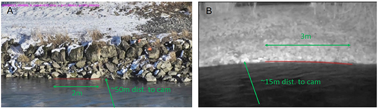
Figure 1. Water level detection, (A) by analyzing changes in texture, (B) by using gray scale.
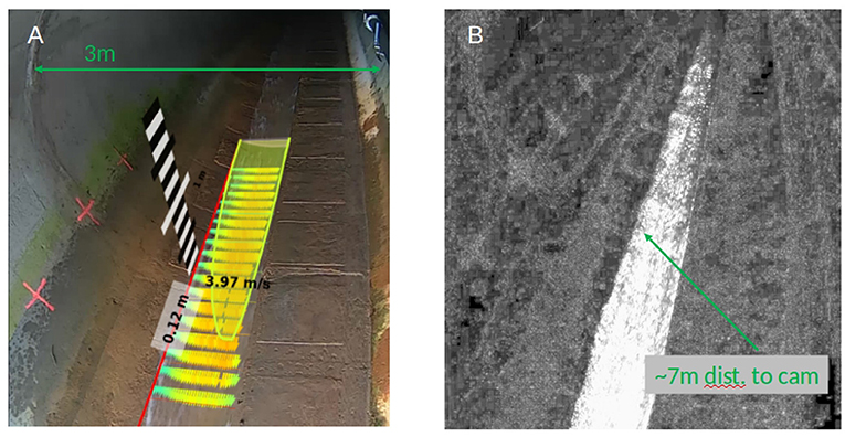
Figure 2. Water level detection by segmenting the moving-non-moving image contents.
The accuracy of the methods depend on the type of shore. If a well-defined plane is available e.g., concrete wall or staff gauge is available, a water level measurement with sub-centimeter accuracy is possible, given sufficient pixel/cm resolution at the shore. For this the camera has to be close to the wall, or the camera has to have enough zoom.
If the river bank is ill defined (as in the case with the boulders in Figure 1A, the accuracy of the optical water level measurements will be more of the order of a few centimeters, scaling e.g., with the size of the boulders. In some further cases, an optical water level measurement is not possible at all. This is mostly the case when the river banks are ill defined (e.g., the shores are not straight), due to vegetation that blocks the direct view to the shore, or because no banks are located within in the field of view. In such cases, the use of an external water level sensor such as level radar, pressure or bubbler sensors is required. External sensors can be connected to the DischargeKeeper which will control and synchronize its functioning.
Surface Velocity Calculation
Once the correspondence between image space and object space has been established via camera calibration, the images are orthorectified and at the same time, if desired and/or necessary, corrected for lens distortion. Then an image velocimetry algorithm is applied to calculate the surface displacements. The main algorithm used is the Surface Structure Image Velocimetry (SSIV) (Lüthi et al., 2018) which is a variation of image velocimetry techniques, it is based on a cross correlation technique and has a number of features in common with LSPIV. SSIV is designed for operational use and tries to overcome some of the known factors that compromise LSPIV performance (i) glare and shadows on the water surface, and (ii) lack of traceable features in the flow (Muste et al., 2008). With these improvements, SSIV is very robust in challenging conditions as showed by Leitão et al. (2018). SSIV is also used in the smart-phone application “Discharge” (Lüthi et al., 2014; photrack, 2017; Peña-Haro et al., 2018; Fehri et al., 2020). Hansen et al. (2017) showed the good performance of SSIV in measuring flow velocity in a continuous manner in3different applications: a 30 m wide river, a channelized river and a channel in a wastewater treatment plant.
SSIV applies a filter to the images prior the cross correlation in order to reduce the influence of glare and shadows and to enhance structures that are present on the free flow surface. SSIV applies a simple image subtraction process, in which the images are subtracted by an image created from a set of temporal averaged images and by applying a Gaussian filter, as described in Lüthi et al. (2018).
All frames to be analyzed are subdivided in interrogation windows on which the cross-correlation algorithm is applied, yielding a displacement field. This displacement field with pixel per frame units can then be converted into a metric velocity field with units meters per second.
Figure 3A shows an orthorectified image and the interrogation windows used for the surface displacement calculation for the site described earlier. Figure 3B shows a so-called “proof-image” of this measurement, with the detected water level and a virtual gauge, the surface velocity field and the resulting velocity profile. Note how the orthorectification of the image is performed only for the part covered by the water surface, so that in effect it is substantially cropped with respect to the original image.
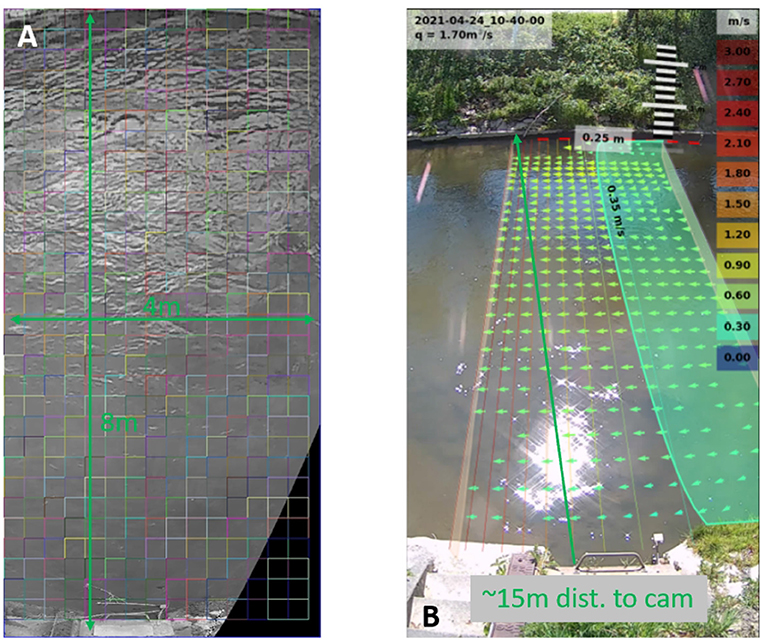
Figure 3. Orthorectified image with the interrogation windows used (A). Proof-image, summarizing the results of a measurement augmented with a virtual staff gauge (B).
The code is written in C++ and care has been taken to optimize it and to make use of multiple cores. The algorithm can process a measurement in >1 min in a smart-phone with the DischargeApp (photrack, 2017).
LSPIV methods are not recommended for shallow angles, which makes it necessary to install cameras at high position, which is not always possible. For these situations Space-Time Image velocimetry (STIV) (Fujita et al., 2007) can be applied. STIV also allows to measure in situations with very fast velocities and under-sampled video material. It must be noted that STIV is one-component measurement method in the stream-wise direction, hence it should not be applied on flows which have significant lateral components. Further, the method relies on strong and most of all on long lived features on the water surface.
In order to have a robust and versatile system, STIV has been integrated into the DischargeKeeper, with some modifications. STIV as described in Fujita et al. (2007) needs to define searching lines to create the space-time image, in our case the field of view is equally divided. Instead of defining lines the users may specify the number of rows in which the image should be divided. The user can further define over how many lateral pixels those lines should be averaged and how long the lines should be. Once the space-image is created (e.g., Figure 4A) the velocity is determined by measuring the prevailing pattern inclination, which is done by creating a 2D auto-correlation function, as e.g., shown in Figure 4B. Figures 4C,D show the final STIV results.
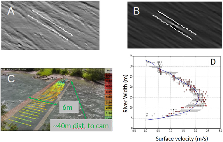
Figure 4. STIV implementation in the DischargeKeeper. (A) Space-time image for a given window. (B) Auto-correlation and line defined. (C) Calculated velocity vectors. (D) Velocity scatter.
Surface Velocity Vectors Filtering
Velocity vectors from the cross-correlation can be erroneous because of wrong matching patterns, or in the case of STIV because wrong detection of the prevailing pattern inclination. In the DK, the erroneous vectors are filtered in two steps. In a first step each velocity vector is compared with up to 8 neighbors, if the vector deviates significantly in direction and magnitude from the 8 neighboring vectors, then it is simply discarded, this is called local filtering. The second filtering is called global filtering since each velocity vector is validated by checking if its magnitude and direction does not deviate significantly from the global mean. Filters can be turned off, for example when 2D flows are to be measured e.g., cases with significant recirculation zones.
Surface Velocity Profile
The resulting velocity vectors after the filtering typically spread across the transect, and where this is not the case, it is possible to interpolate or extrapolate measurements using polynomial, cubic, or the constant Froude method (Perks et al., 2020), however our methodology follows a different approach. A velocity profile is fitted to the stream-wise components of the measured velocity field. One assumption made here, is that the flow is in steady-state within the region of interest. The flow field data is collapsed along the stream-wise axis. Surface velocity profiles of rivers may, depending on the geometry of the cross-section, be symmetric, asymmetric, the profiles may vary in their bulkiness or they may even exhibit recirculation zones with negative velocities. Different implementations of the velocity profile fit allow to cope with these different situations. While fitting the envelope to the data a third filter is applied, data points that are far (this parameter can be adjusted) from the optimal envelope are discarded and not use for the fit, hence fitting the surface profile is an iterative procedure. The raw data is plotted as gray circles and the data retained after the filtering is shown in red. The blue line shows the final fit obtained with the filtered data and the gray bar represent the uncertainty of the fit for a given span-wise position (Figures 4, 5).
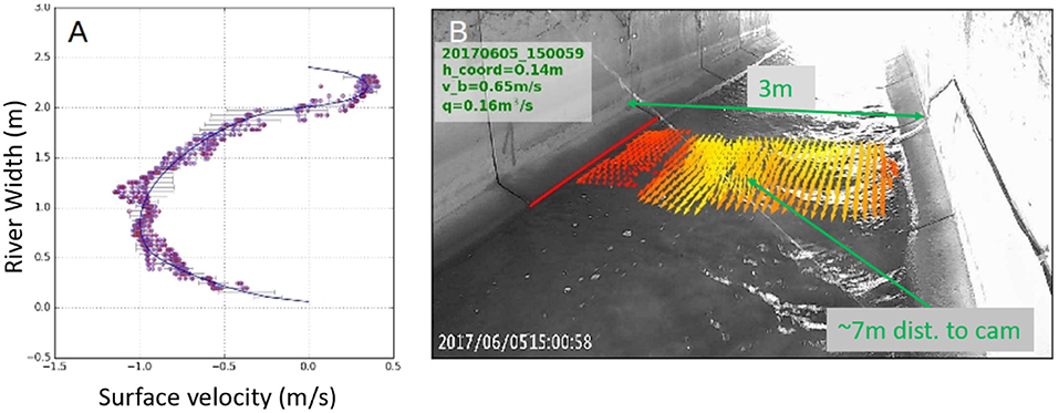
Figure 5. (A) Scatter plot of surface velocities vs. river width (on the right shore the back flow can be seen). (B) Velocity vectors, it can also be seen the back flow, red line shows the result of the optical water measurement.
Monitoring stations should be installed in places where there are no changes in cross section and in straight stretches of the river/canal to avoid no-uniform flow. However, sometimes reality has less well-behaved flow profiles and for this reason we allow the surface velocity profile to accommodate those type of flows that are produced in such conditions, like back-flow (Figure 5).
The surface velocity profile is fitted to the velocity x-component using 4 parameters or 6 in the case of back flow, hence the surface velocity can be modeled by using only those parameters. This opens many possibilities, like making temporal comparisons of the variation of the flow patterns and identified changes on it. Some of those changes can be created by changes in the cross-section, hence it is automatically detected when the cross-section should be updated.
Figure 6A shows the velocity vectors resulting of a single video processing and Figure 6B shows the corresponding surface velocity envelope, where the thin blue line denotes the 4 parameter curve fit to the measured velocities of the each sub-window.
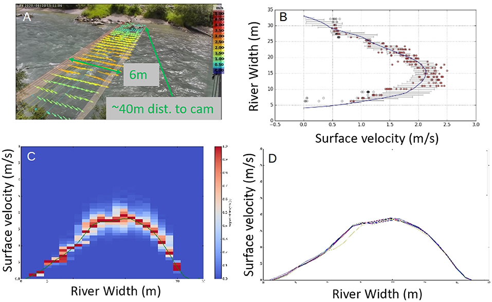
Figure 6. (A) Surface velocity field. (B) Surface velocity envelope for one video. (C) Ensemble of 107 envelopes at the water level ±0.1 m. (D) Comparison of surface velocity ensembles at different dates.
If these velocity profile results are collected over some time, here we present a statistic over 2 months, the velocity profile can be monitored and questions relevant for site maintenance can be asked; does the velocity profile stay constant for a given water level? Does the velocity profile change? If the change is persistent, does it point to a bed mobilization? In Figures 6C,D we present results to indicate how this may look. Figure 6C shows the mean velocity profile for a given water level h = 614.7 m collected over a 2 week time period t and included into the set whenever the water level was ±10 cm close to the targeted h = 614.7 m. The color coding indicates the relative probability distribution of the surface velocities. The thin green line is the resulting mean surface velocity profile conditioned on h and t. This procedure is repeated 8 times distributed over the observation period of 2 months. The resulting mean surface velocity profiles <v>|(h,t) are then plotted in Figure 6D. It can be seen that all curves more or less collapse. This is indicating that the surface velocity profile (i) has remained stable throughout the observation period and (ii) that the mean surface velocity profile is well-converged. The shape of the such learned velocity profiles can now be used to enhance individual measurements by computing the discharge with these “learned” and fully converged velocity profiles as compared to the parametrized profiles.
Depth Averaged Velocity and Discharge Computation
Once the surface velocity profile is obtained, and given that the bathymetry of the stream is known as well as the river stage, it is then possible to calculate the discharge by integrating the depth-averaged velocity over the width of the river. Several approaches, from physically-based models to fully empiric models, are available to perform this task. A physically-based approach would be to extend the mixing length model, as defined by Prandtl, to account for the influence of the wall roughness (here river bed roughness) on the vertical velocity profile, as described in Absi (2006). Another approach would be to follow the guidelines edited by the ISO (2007) accounting for the river bed roughness by using a Manning roughness. However, as in most cases the depth-averaged velocity is calibrated with experimental data, many practitioners decide to follow an approach based on the commonly named alpha (α) value expressing the ratio between the depth-averaged velocity and the surface velocity. Hauet et al. (2018) investigated the dependency of the α value on roughness and slope in a study performed while considering more than 3,000 gaugings obtained from more than 175 different French rivers. These authors showed with a confidence interval of 90% that for sandy, pebbly or boulder rivers at low flows, the α value is of 0.8 with an uncertainty range of ±15%. These authors also reported that the α value could increase up to 0.9 for higher water levels by apparently following a linear trend. This is a very good approximation to start with, but can lead to substantial errors in the discharge computation in some cases. This is particularly true when the roughness is heterogeneously distributed over the river bed or the river banks and foremost when secondary currents may cause subsurface velocity dips (Nezu et al., 1993) that would not be recognized by a technology only sampling the water surface. However, in such cases, the α-value may vary over a larger range and be a non-linear function of the water level. Using the latest advances in numerical modeling (Talebpour and Liu, 2019), it may soon be possible to define this α value–water level based on numerical results taking both the slope and the roughness into account, possibly further decreasing the uncertainty of this conversion factor.
Multi-View Systems
If the camera is located at shallow angles with respect to the horizontal, the image resolution and image quality will be compromised at the far field, which can introduce errors in the calculation of the surface velocities. A tilting angle of 10° was found to be the acceptable limit (Muste et al., 2008). If we consider that the camera is mounted at one of the river shores, this means that for large rivers, the camera would have to be mounted very high to keep the minimum angle, which is not always feasible. However, there are some alternative approaches to image also larger rivers. It was shown by Bechle et al. (2012) that with multi-view systems it is possible to extend the application range of image velocimetry techniques to large rivers. To do so, these authors used multiple cameras to measure multiple views.
The DischargeKeeper can be equipped with Pan-Tilt-Zoom (PTZ) cameras. The use of PTZ cameras can significantly help to overcome some limitations related to the camera positioning and to avoid disadvantageous points of view. The main idea is to use the camera capabilities to focus to smaller sections of the river (Figures 11C,D), as it can be seen on those figures, there is no visible shore where to position GCP's, therefore a new procedure for camera calibration was developed. This procedure consists on calibrating the camera mount position, orientation and the relation between zoom and focal length of the camera. Then by obtaining the pan, tilt and zoom values from the stepping motors, the camera views can be calibrated (Peña-Haro et al., 2021). An example of this implementation is show in the site section.
Hardware
Cloud or Edge Solution
When it comes to the hardware, it is possible to distinguish between cloud or edge solution. In some cases, when the water level can easily be measured optically, when Internet connection is available and when vandalism may be an issue, choosing a cloud solution may be an appealing option. In such a case, the camera would just continuously upload the data to the cloud. Then, upon arrival, the video sequences are being analyzed automatically. Such a cloud solution can be implemented on local national cloud services, which may be required by countries where water data is sensible and cannot exit the country. An edge solution follows a completely different approach. In such a case, a complete instrument device consisting of a camera and a cabinet containing a central unit, an uninterrupted power supply, a power over Ethernet injector, a router etc. is installed on site. The entire data processing is done on site on a central unit, whose energy consumption can be supplied by a solar panel. Such as system is typically transmitting only the final results, optionally it may be configured to also transmit raw data at a configurable frequency. Depending on the use case, any combination of both, edge or cloud solution, is technically feasible.
Camera
The camera is the key component of the DK continuous measurement systems. Depending on the use case, so-called bullet or PTZ cameras can be used. It is important that the camera does not compress the video too much when looking at water scenes with fairly homogeneous colors. Too strong image compression would not allow to detect the surface structures. If the system is installed in a potentially explosive environment, cameras compliant with the ATEX directive should be employed. As shown in Leitão et al. (2018), for the SSIV technology, the temporal resolution (frame rate) is more critical than the spatial resolution. Typically, HD resolution (1,920 × 1,080 @ 30 fps) allows to obtain satisfying results, as most visible but short lived surfaced structures persist for at least O(0.1) s.
Central Units
The central unit (for edge solutions) consists of an industrial PC that performs the image processing and further data analysis on site. Typically, a small industrial PC with a processor of 4 × 1.5 GHz, 3.7 GB RAM and a hard drive of 128 GB is adequate for the processing and for local data storage. Some industrial PCs support integrated watchdog timers that can enhance their reliability. Additionally, integration of a 3G/4G modem within the central unit can allow to provide a stable and reliable wireless connection to available networks.
Router
Depending on the use case, it can be necessary to have the watchdog functionality and the wireless connection covered by an external router or to have an additional redundancy concerning these features. Further, an external router facilitates direct access to the camera live-stream via fixed IP address.
External Level Sensors
If the optical water level detection is not possible or if redundancy is required for that measurement, the use of an external water level sensor, such as level radar, pressure sensor, or bubbler sensor, may be considered. Values obtained from such a sensor can be passed over an analog-digital converter (e.g., 4–20 mA), a serial digital interface (SDI) or over a Modbus interface, depending on what data transmission technology is available. Additionally, it is also possible to continuously fetch the water level from a server, a website or an application programming interface (API) if the value is available online.
Smart Power Module
The system can be powered by 12 V and in order to make efficient use of the available and typically limited battery power, the so called “smart-power module” was developed. This device is an intelligent switch for each of the system consumers and it allows to adjust the measurement interval depending on the battery voltage and on the flow conditions. For example, if there the water level is raising and/or if the velocity is changing the measurement interval will be made shorter. If the flow is constant the measurement interval will be longer. The module powers the peripherals exactly only when they are needed and shuts them down, if immediately after their usage.
Results Transmission
The DischargeKeeper can send the results using any state-of-the-art technology, be it analog, SDI, Modbus, ftp server, API, etc. The transmission frequency is configurable for each data type, such as values for level, velocity and discharge, images, or even raw input videos.
Data Visualization
The DischargeKeeper, when desired, can send the measurements to the DischargeDataHub (discharge.ch) which is a data visualization web-platform. The DischargeDataHub allows to scroll through DK data, consult the proof images of every measurement, set real-time alarms on the different variables and generate rating curves.
If the DK Internet connection, the DischargeDataHub can also be used to modify the main parameters of the DK remotely, without the need of going to the field.
System Robustness
In the previous sections the main components and algorithms implemented in the DischargeKeeper have been explained. In this section, we describe how those components have helped the system to improve the overall system robustness and thereby reaching a Technology Readiness Level (TRL) of 9.
The quality and accuracy of the field work is key to high overall quality of the discharge measurements, therefore the calibration process was simplified as much as possible. Initially, we required 6 or even more ground control points (GCP) for camera calibration. With the current system only 2 GCPs plus the position of the mounted camera need to be measured in by the ground survey staff. This new calibration procedure saves time in the field and reduces potential sources of errors, while maintaining highly accurate camera calibration.
The presented DK system integrates several optical water level measurement methods with the signal of external level sensors. The DK can obtain the water level exclusively optically or from external sensors, or the DK can be configured to use optical methods as a fall back plan, should the external signal fail, due to component damage. Unlike other optical measurement solutions, the here presented DK system does not need an artificial object in its view, i.e., it is not necessary to mount staff gauges or similar. Sometimes, the shorelines is obscured by plants, or illumination conditions result in a very dark waterline image region. For such situations a so-called velocity index matching algorithm has been developed, which determines a robust first estimate of the water level. Naturally this method may only be employed for situations with stable surface velocity–discharge relations.
With our standard technique SSIV for determining water surface velocities, we have a robust approach also for situations with weak signal, due to small surface roughness, and for situations with hard illumination changes across the field of view, mostly caused by time-evolving shade patterns of trees, bridges or similar. As an additional measure to enhance robustness, the known approach STIV has been adapted for the DK system. We find that it allows to measure in situations with very fast velocities and under-sampled video material. A significant increase of additional robustness was achieved by proper filtering of sub-window velocity measurements and their successive fitting to suitable velocity profile base curves. The base curves are defined by 4 parameters, 6 if also backflow situations are covered.
The individual surface velocity measurements are stored in an internal database with respect to their corresponding water levels. This is equivalent to saying, the DK system is “learning” the velocity profiles for given water levels. This approach is adding another layer of robustness, as outliers can be detected in a more straight forward manner. With the accumulated velocity profiles for given water levels, the DK system is building its internal rating curve, i.e., it is “learning” it. If the learned rating curve is departing significantly from the original rating curve, this is serving as a robust indication for a so-called de-rating event, and successively a configured list of people may be informed and warned via automatic emails or sms.
Further, if an individual measurement is deviating too much from the current operational rating curve, then the measurement may be corrected toward to more likely rating curve value. At the same time however, the measurement is marked as “corrected,” and if the correction is occurring systematically over a significant period of time, a defined list of users is informed via email or sms.
All the above mentioned measures result in improved robustness of individual components of the DK system. In the following we will report some additional measures aiming at monitoring the functioning of the components, but also the interplay between the components.
Each of the above explained algorithms is running on the PC as a stand-alone instance. An overarching script is monitoring their proper functioning and, if needed, is killing and restarting the processes. This guaranties that the entire DK system is not “taken down” by the failure of a single component. In a similar way, the proper functioning of the connected camera is monitored, and if needed the camera is rebooted. Finally also the PC is being watched, either by a watchdog configured on the BIOS level of the PC or by the connected router, which, if needed operates a relays to trigger a OFF/ON cycle of the PC. Naturally, in the case where the DK system is controlled by the Smart Power Module, typically for each measurement cycle the components are switched ON, which is resulting in increased system stability–at the price of slightly lower measurement frequencies, as compared to a continuous DK system.
The DK is storing most of the relevant results locally, even when they are not planned to be transmitted to the customer data storage. This storage is organized in a ring memory fashion, i.e., according to the total storage capacity, data is kept for a few days, or even for a few weeks before it is deleted for good. This adds robustness, as the customer can always go and physically collect the recent data directly from the system. The final results, such as values for water level, surface velocity, discharge rate, proof images, or even measured video sequences are transmitted to a standard or customized data base. Typically, data transmission is performed over mobile network, and it is thus vulnerable to some occasional technical failures. The DK system is packaging the “to be transmitted” data into tickets. Only if a transmission is confirmed as successful, those tickets are removed. If a transmission has failed, the transmission attempts are repeated at regular intervals. This approach ensures that all data ultimately is transmitted to the data base, if transmission is not possible, the tickets are managed to not saturate the system.
Based on our experience, it is not a single individual measure, but it is the sum of all above mentioned measures that have resulted in an overall TRL increase for the DK system from <7 to 9, i.e., the DK system has evolved from a reliable tool for individual measurements to a robust system, capable for maintaining a 7 × 24 operational mode all year long for a wide range of real world free surface flow situations.
Case Studies
In the following, 3 different sites for which data has been gathered for several years are presented, serving as case studies showcasing possible issues to be faced during long term operation of image velocimetry systems.
Measurement System in a Harsh Alpine Environment
Site Description
The following measurement system has been installed for 6 seasons to measure glacier melt discharge below the tongue of a glacier in an alpine canyon. The system is mainly solar powered, but a fuel cell takes over when the sunlight does not allow to completely cover the energy consumption. The left panel in Figure 7 depicts the scene in which this system is installed. The cabinet with the solar panel is located at the right of the bridge, top right corner of the image. The camera and a visible light LED beamer are mounted directly on the rock below the bridge. In this canyon, entering the stream is not possible as flow velocities can reach up to 6 m/s. Therefore, the bathymetry was obtained using a photogrammetric method, structure from motion with 6 measured in ground control points, that allowed reconstructing the scene with multiple images acquired with smart-phone cameras under very low flow conditions. The roughness of the bathymetry was calibrated using reference measurements performed with chemical tracers. The system measures at an hourly interval under day and night conditions.
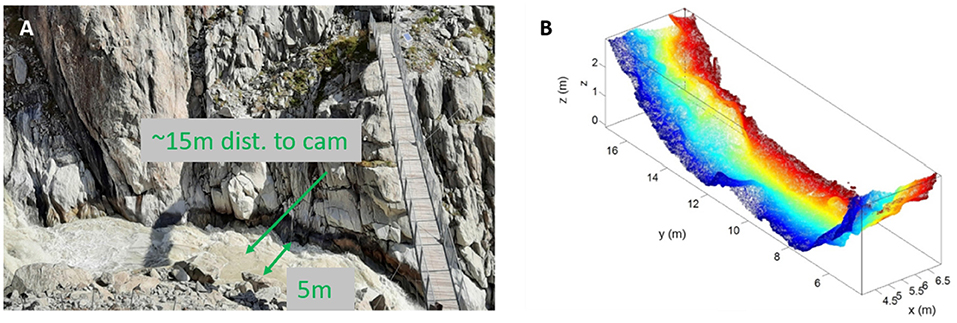
Figure 7. Image of the alpine canyon in which the measurement system is installed (A). Bathymetry of the site obtained from photogrammetry, color-coded with the stream-wise position (B).
Influence of Erosion on the Measurements
The daily flow measured during the seasons 2015–2020 is shown in Figure 8. The high variability of these time series shows the fast reaction of the stream catchment to rainfall events. Some of the massive events can be explained by rainfall on accumulated snow-pack resulting in important discharges. Note that the measurement system is removed over winter due to risks linked to avalanches and reinstalled once that the measurement site is snow free. The season-to-season variations in snow cover explain the different lengths of the seasonal time series, e.g., for some seasons the system has to be removed earlier while for some others, its installation has to be postponed because of the delayed snow melt at site.
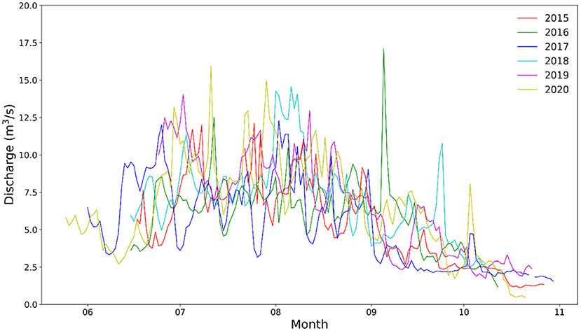
Figure 8. Daily stream-flow discharge rate, <q>|day, measured for the snow-melt seasons of 2015–2020 at this site.
Due to the glacier withdrawal and permafrost melting in the vicinity of the measurement site, this stream has an important sediment load and is prone to important events of hydromorphological nature. This was particularly true for the season of 2018. First, at the beginning of August 2018, significant rainfall events resulted in sustained high flows (Figure 8), that modified the cross-section of the site. This was revealed by a so-called de-rating of the site, meaning that upon this event, the relationship expressing the dependency of the discharge on the water level changed. For many streams, the relationship between the water level and the discharge can be well-described by a function (often a power law), as so-called a rating curve. The de-rating event during calendar week 31 of the year 2018 is well-visible on Figure 9A. Note that the cross-section of the site had to be recalibrated after the de-rating event and allowed to correct the data (data not shown). This de-rating event highlights an interesting feature of this image-based technology, namely, the fact that the measurements are always obtained from two independent variables. Pressure gauges are commonly used in alpine environments and the discharge is then obtained using rating curves, such an event would have gone unnoticed. The 2019 data illustrated on Figure 9B does not exhibit any de-rating events. This figure also shows the results of chemical tracer tests performed, the relative error related to the tracer test was 6.3% which are well-located within a 10% uncertainty range added to a rating curve obtained by fitting a power law to the measured data in a least squares sense.
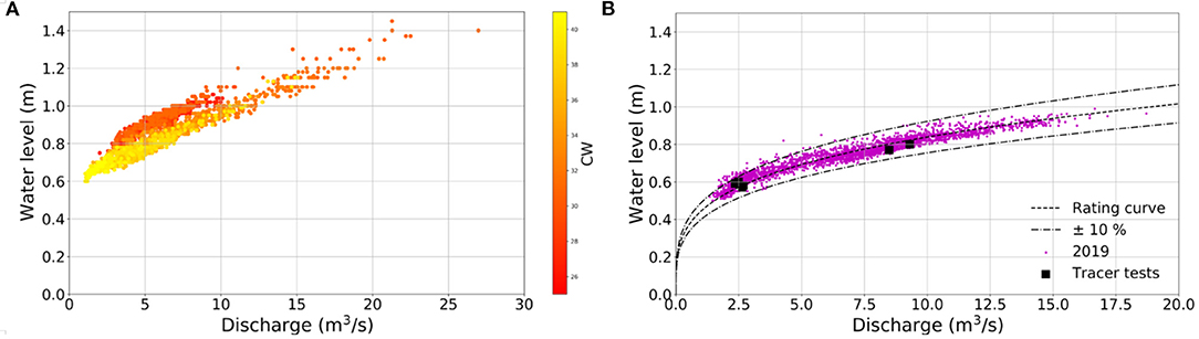
Figure 9. Water level and discharge data measured for 2018 (A) and for 2019 (B).
Another interesting feature of image-based technologies for discharge measurements is the visual control that can be easily performed on the measured data, ultimately allowing to perform plausibility checks on the measured data. In this specific case, it was possible to detect a massive rock block on the field of view leading to a new configuration of the site.
Measurements on a Large Alpine River
The next site is at the Rhine river at the border between Switzerland and Austria. At this location the river is around 100 m wide and the flood plain is about 200 m. There is an important hydro-power activity in the catchment of this river which produces fluctuations on the flow. In this site a PTZ camera was installed under a bridge (Figure 10) and the discharge calculation is done using a multi-view approach.
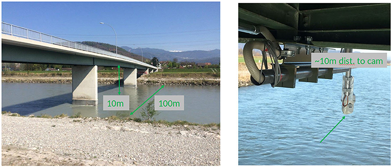
Figure 10. Site location and PTZ camera.
Velocity views are defined in order to capture the entire width of the river, allowing to obtain truly spatially resolved measurements on such a large river (Figures 11C,D). Additionally to the velocity views a dedicated view to optically measure the water level was defined (Figures 11A,B).
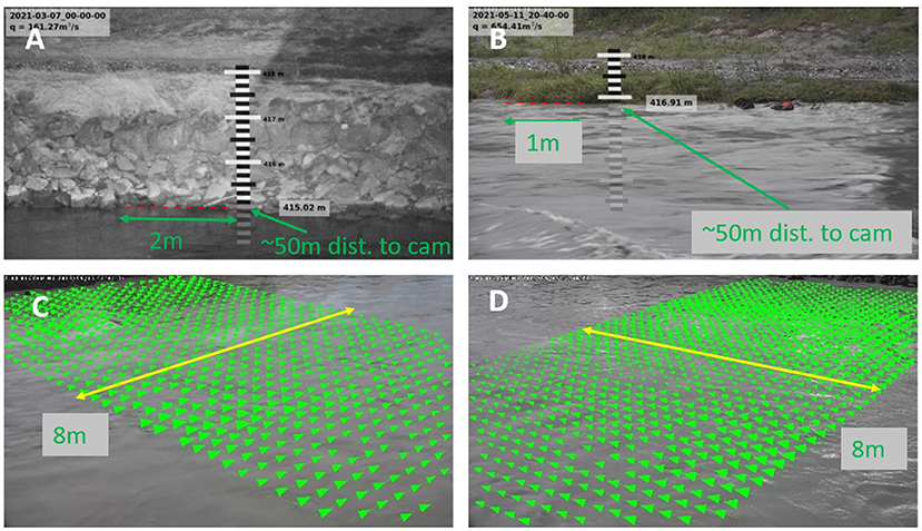
Figure 11. Defined views (A,B) level view, (B) measurement taken at night. Side velocity views (C,D) as obtained with a PTZ camera in Montlingen.
The camera has an integrated infrared beamer that, according to the manufacturer's specifications, should illuminate objects that are located as far as 250 m away of the camera under night conditions. Testing of this camera however revealed that, while the specifications may be true for surveillance purposes, the illumination was not good enough to reliably record the displacement of tiny features like surface structure and hence, night velocity measurements were not possible at large distances > ~20 m. In order to overcome these limitations, a dedicated view was defined in a region where the distance to water was about 10 m and where the IR illumination is good enough to detect accurately surface structures at night. However, this view does not cover the whole river with but only a smaller part of it. For night measurements the parameters of the surface velocity profile are those of the ones estimated during the day. If necessary, additional external infrared beamers can be added to enhance the illumination at night.
A 6 weeks long time series of 10 min interval discharge measurements obtained with the DischargeKeeper and with a radar located on the same bridge are displayed in Figure 12.
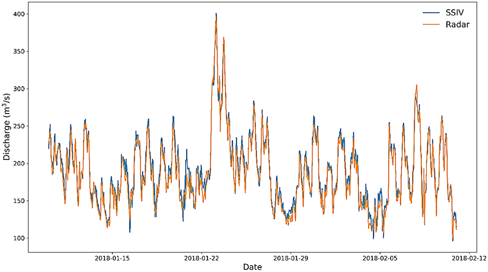
Figure 12. Discharge time series for 6 weeks of continuous measurement during which a radar measurement was also available for comparison.
It can be seen the effects of the hydro-power activity on the high dynamic range exhibited by these time series. The correspondence between both measurement systems is very good, for high flow as for low flows. During the analyzed period, the mean discharge was of 190 m3/s and the root square mean error (RSME) was of 8.49 m3/s. The RMSE for the optically measured level was of 0.068 m.
Measurements on a German Mid-Size Stream
A DischargeKeeper was installed in 2019 at the Peissenberg monitoring station on the Ammar River in Southern Germany. At this site a bullet camera and an external infrared beamer where installed (Figure 13), the river stage is measured using an external level sensor. The system continuously takes measurements every 2 min. Figure 13 shows the result images with measured values and timestamps at different flow conditions for the site Peissenberg.
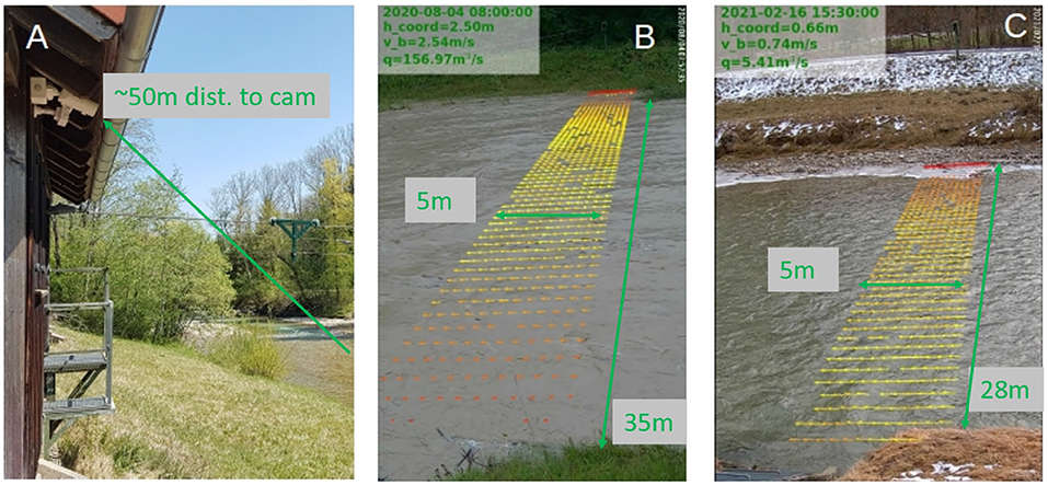
Figure 13. Discharge measurements for different conditions, (A) low flow, (B) high flow, (C) ice at the shore.
Comparison between the DischargeKeeper and reference measurements carried out under different flow conditions, which taken with ADCP, Radar and electromagnetic current meter. The relative deviation between the reference measurements and the DischargeKeeper measurement was 10.4%, specifically the error between the ADCP and the DischargeKeeper was of 3% (Figure 14).
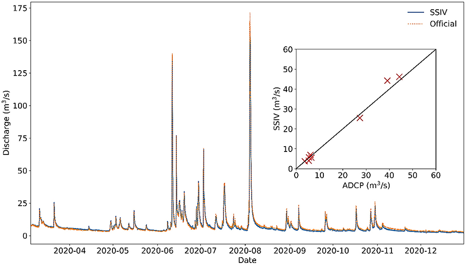
Figure 14. Comparison of Discharge measurements between SSIV and official values. In the small box comparison between SSIV and ADCP.
A flood event occurred in May 20th, 2019 that statistically corresponds to a 5–10 year event. A flow measurement with a measuring blade or ADCP boat would not have been possible at that time due to the large quantities of wood drift. Having a no-contact, camera-based system, the measuring of flow velocity, and flow rate was possible unimpaired even during the flood event (Hansen et al., 2020). The flood peak discharge measured with the DischargeKeeper was ~176 m3/s, for comparison, the measured value of a mobile discharge radar measurement was 175 m3/s. Thus, the agreement between the DischargeKeeper data and the reference measurement data could be described as very good with <1% relative deviation.
Discussion
The DischargeKeeper is a mature system which has a Technology Readiness Level 9: “Actual system proven in operational environment.” The system has reached that TRL, by increasing the robustness of each its components -hardware and software-, but more importantly, by improving the robustness of the interplay of these features and by adding systems to monitor each of the components.
The DischargeKeeper has been installed in many different rivers and canals ranging from 40 cm to 100 m, proving that the system is robust. In this paper three cases are shown in more detail. The first one, an alpine river, where the DischargeKeeper is supplied with a battery and it is located in a remote area. The area is protected by UNESCO; hence the system has to have minimum impact. The system has been running for 6 years, during this time several tracer test have been performed showing a relative error of 6.2%. The second case is 100 m wide river, where a multi-view DischargeKeeper was installed. The system is optically measuring the water level. The error against the official values for the analyzed period was of 3.5%. The third case, is a medium size river in Germany, it has grid power and Internet connection. The water level is measured via a radar. It has been compared against ADCP/propeller measurements having an error of 10.4%.
Despite all the merits of the existing operational DischargeKeeper, some areas of further development remain:
- Water level. Not all rivers are suitable for measuring the water level optically. For optical level measurements, care must be taken to keep the shore free of vegetation. However, external sensors can be added. Ongoing internal research is aimed at developing a suitable Artificial Intelligence (AI) optical level module. It is trained with the complete outputs of all available approaches and their corresponding correct water levels, to learn how to take intelligent decisions, i.e., which signal for the current conditions is the most reliable for water level detection.
- Velocity measurements. Under very low flow conditions, at velocities below 0.2 m/s typically visible surface patterns cease to exist. However, if the river stage can be measured, rating curves fitted to measured values can be used to estimate the discharge.
- Surface velocity profile. It is based on 4 parameters or 6 if also backflow situations are covered. The current approach is yielding robust results, but also here we note the high potential of AI for choosing exactly which sub-window measurements should be used for velocity profile fitting.
- Night measurements. Artificial illumination, either infrared or visible light, has to be mounted for night measurements and aligned properly onto the cameras field of view. This is a limitation in wide rivers where the illumination is difficult. In such cases the velocity is measured in a small area and the learned parameters during the day of the velocity envelope are used to fit the surface velocity envelope to the measurements during night.
- Wind can have a strong effect on the surface velocity, especially in slow flowing rivers. Wind can be easily measured and detected and thus discard measurements affected by it.
- Depth average velocity. Even though several models have been implemented, to accurately model complex flow situations remains a challenge. This is especially true when secondary currents are present due to high aspect ratios of depth over flow width, or due to significant roughness changes along the cross sectional profile. More elaborate numerical modeling is being under development and will be communicated in dedicated future note.
Conclusions
With the presented DischargeKeeper a continuous optical measurement system has been developed which has a 7 × 24 operational capability for a variety of stream types and flow conditions, i.e., to a TRL level of 9. This development has been made possible because a combination of several factors, reliable sensitive IP cameras with good resolution, low pixel noise at modest prices, robust image velocimetry algorithms (SSIV and STIV) which are fast enough to allow quasi-real time measurements, optical water level detection algorithms and the possibility to connect external sensors and synchronize their measurements with the video recording. A crucial contribution to a TRL 9 level, is the robust interplay of all these improved components and there self-checking algorithms, which can trigger reboots and re-starts. Different type of cameras allow to monitor canals of a couple meters width to rivers of more than 100 m width. The DischargeKeeper has the capability to run on the edge or in the cloud and to transmit the measurements in analog or digital form. The presented system has been installed in more than 50 rivers and canals around the world, proving its reliability in daily operational conditions.
However, several development challenges remain. It still proves difficult to measure under certain environmental conditions, mainly during low visibility (night, fog) but also under strong winds. The advent of cameras that are even more light sensitive will soon ease the former challenge. Another field of developments the calculation of the depth averaged velocity. The DischargeKeeper has several models implemented, but for complex flows, especially when secondary currents are present, key assumptions of these methods are no longer valid and either empirical gathered correction factors or numerical simulations have to be employed to further increase the accuracy of the DischargeKeeper.
Data Availability Statement
The datasets presented in this article are not readily available because data belongs to third parties. Requests to access the datasets should be directed to cGVuYUBwaG90cmFjay5jaA==.
Author Contributions
SP-H: paper conceptualization. BL and SP-H: system development. MC, SP-H, BL, and IH: data analysis. MC, SP-H, BL, IH, and RL: writing and editing. All authors contributed to the article and approved the submitted version.
Funding
Initial funding was provided by a BAFU research project with photrack. Additional funding has been provided by SEBA Hydrometrie.
Conflict of Interest
The system has been developed with funding from BAFU and SEBA Hydrometrie. SP-H, BL, and MC work at photrack and IH at SEBA Hydrometie.
The remaining author declares that the research was conducted in the absence of any commercial or financial relationships that could be construed as a potential conflict of interest.
Publisher's Note
All claims expressed in this article are solely those of the authors and do not necessarily represent those of their affiliated organizations, or those of the publisher, the editors and the reviewers. Any product that may be evaluated in this article, or claim that may be made by its manufacturer, is not guaranteed or endorsed by the publisher.
Acknowledgments
The authors want to thank the BAFU for providing ideas for the system improvement and facilitating data.
References
Absi, R. (2006). A roughness and time dependent mixing length equation. J. Hydr. Coast. Enviro. Eng. 62, 437–446. doi: 10.2208/jscejb.62.437
Bechle, A., and Wu, C. (2011). Virtual wave gauges based upon stereo imaging for measuring surface wave characteristics. Coas. Eng. 58, 305–316. doi: 10.1016/j.coastaleng.2010.11.003
Bechle, A. J., Wu, C., Wen-Cheng, L., and Nobuaki, K. (2012). Development and application of an automated river-estuary discharge imaging system. J. Hydr. Eng. 138, 327–339. doi: 10.1061/(ASCE)HY.1943-7900.0000521
Carrel, M., Martin, D., Peña-Haro, S., and Lüthi, B. (2019). “Evaluation of the dischargeApp: a smartphone application for discharge measurements,” in Hydrosensoft, International Symposium and Exhibition on Hydro-Environment Sensors and Software (Madrid).
Detert, M., and Weitbrecht, V. (2015). A low-cost airborne velocimetry system: proof of concept. J. Hydr. Res. 53, 532–539. doi: 10.1080/00221686.2015.1054322
Dramais, G., Le Coz, J., Camenen, B, and Hauet, A. (2011). Advantages of a mobile LSPIV method for measuring flood discharges and improving stage–discharge curves. J. Hydro-Environ. Res. 5, 301–312. doi: 10.1016/j.jher.2010.12.005
European Commission (2014). Technology readiness levels (TRL); Extract from Part 19 - Commission Decision C(2014)4995. Available online at: https://ec.europa.eu/research/participants/data/ref/h2020/wp/2014_2015/annexes/h2020-wp1415-annex-g-trl_en.pdf (accessed November 29, 2021).
Fehri, R., Bogaert, P., Khlifi, S., and Vanclooster, M. (2020). Data fusion of citizen-generated smartphone discharge measurements in Tunisia. J. Hydrol. 590:125518. doi: 10.1016/j.jhydrol.2020.125518
Fujita, I., and Kunita, Y. (2011). Application of aerial LSPIV to the 2002 flood of the yodo river using a helicopter mounted high density video camera. J. Hydro-Environ. Res. 5, 323–331. doi: 10.1016/j.jher.2011.05.003
Fujita, I., Muste, M., and Kruger, A. (1998). Large-scale particle image velocimetry for flow analysis in hydraulic engineering applications. J. Hydr. Res. 36, 397–414. doi: 10.1080/00221689809498626
Fujita, I., Watanabe, H., and Tsubaki, R. (2007). Development of a non-intrusive and efficient flow monitoring technique: the space-time image velocimetry (STIV). Int. J. River Basin Manag. 5, 105–114. doi: 10.1080/15715124.2007.9635310
Hansen, I., Daamen, K., and Peña-Haro, S. (2020). Kamerabasiertes Durchflussmess-verfahren an Fließgewässern - Fallstudie Peißenberg-Hochwasser Mai 2019. doi: 10.1007/s35147-020-0408-9 Fachzeitschrift Wasserwirtschaft. Available online at: https://www.springerprofessional.de/kamerabasiertes-durchflussmess-verfahren-an-fliessgewaessern-fal/18039064 (accessed November 29, 2021).
Hansen, I., Satzger, C., Sattler, M., Lüthi, B., Peña-Haro, S., and Düster, R. (2017). An Innovative Image Processing Method for Flow Measurement in Open Channels and Rivers. Palakkad: flotek.g. India.
Hauet, A., Kruger, A., Krajewski, W., Bradley, A., Muste, M., Creutin, J., et al. (2008). Experimental system for real-time discharge estimation using an image-based method. J. Hydrol. Eng. 13, 105–110. doi: 10.1061/(ASCE)1084-0699(2008)13:2(105)
Hauet, A., Morlot, T., and Daubagnan, L. (2018). Velocity profile and depth-averaged to surface velocity in natural streams: a review over alarge sample of rivers. E3S Web Conf. 40:06015. doi: 10.1051/e3sconf/20184006015
ISO (2007). Hydrometry—Measurement of Liquid Flow in Open Channels Using Current-Meters or Floats. Vol. 748. ISO.
Jodeau, M., Hauet, A., Paquier, A., Le Coz, J., and Dramais, G. (2008). Application and evaluation of LS-PIV technique for the monitoring of river surface velocities in high flow conditions. Flow Meas. Instr. 19, 117–127. doi: 10.1016/j.flowmeasinst.2007.11.004
Le Boursicaud, R., Pénard, L., Hauet, A., Thollet, F., and Le Coz, J. (2016). Gauging extreme floods on YouTube: application of LSPIV to home movies for the post-event determination of stream discharges. Hydrol. Proc. 30, 90–105. doi: 10.1002/hyp.10532
Le Coz, J., Hauet, A., Pierrefeu, G., Dramais, G., and Camenen, B. (2010). Performance of image-based velocimetry (LSPIV) applied to flash-flood discharge measurements in mediterranean rivers. J. Hydrol. 394, 42–52. doi: 10.1016/j.jhydrol.2010.05.049
Leitão, J. P., Peña-Haro, S., Lüthi, B., Scheidegger, A., and Moy de Vitry, M. (2018). Urban overland runoff velocity measurement with consumer-grade surveillance cameras and surface structure image velocimetry. J. Hydrol. 565, 791–804. doi: 10.1016/j.jhydrol.2018.09.001
Lüthi, B., Philippe, T., and Peña-Haro, S. (2014). “Mobile device app for small open-channel flow measurement,” in Proceedings of the 7th International Congress on Environmental Modelling and Software, eds D. P. Ames, N. W. T. Quinn, and A. E. Rizzoli (San Diego, CA).
Lüthi, B., Philippe, T., and Peña-Haro, S. (2018). Method and System for Determining the Velocity and Level of a Moving Fluid Surface. European Union. Available online at: https://patents.google.com/patent/EP3018483B1/en?q=photrack&oq=photrack (accessed November 29, 2021).
Muste, M., Fujita, I., and Hauet, A. (2008). Large-scale particle image velocimetry for measurements in riverine environments. Water Res. Res. 44:W00D19. doi: 10.1029/2008WR006950
Muste, M., Hauet, A., Fujita, I., Legout, C., and Ho, H. C. (2014). Capabilities of large-scale particle image velocimetry to characterize shallow free-surface flows. Adv. Water Res. 70, 160–171. doi: 10.1016/j.advwatres.2014.04.004
Nezu, I., Tominaga, A., and Nakagawa, H. (1993). Field measurements of secondary currents in straight rivers. J. Hydr. Eng. 119, 598–614. doi: 10.1061/(ASCE)0733-9429(1993)119:5(598)
Pearce, S., Ljubiči,ć, R., Peña-Haro, S., Perks, M., Tauro, F., Pizarro, A., et al. (2020). An evaluation of image velocimetry techniques under low flow conditions and high seeding densities using unmanned aerial systems. Remote Sens. 12:232. doi: 10.3390/rs12020232
Peña-Haro, S., Carrel, M., Lüthi, B., Wang, L., Dicht, S., and Leitão, J. P. (2019). Abflussmessungen mittels videos. Einsatz von Webcams Und Smartphones. Aqua Gas 99, 42–45.
Peña-Haro, S., Lukes, R., Carrel, M., and Lüthi, B. (2021). “Image-based flow measurements in wide rivers using a multi-view approach,” in 14th Congress Interpraevent (Norway).
Peña-Haro, S., Lüthi, B., Carrel, M., and Philippe, T. (2018). “DischargeApp: a smart-phone app for measuring river discharge,” in EGU General Assembly 2018 (Viena).
Perks, M. T., Fortunato Dal Sasso, S., Hauet, A., Jamieson, E., Le Coz, J., Pearce, S., et al. (2020). Towards harmonisation of image velocimetry techniques for river surface velocity observations. Earth Syst. Sci. Data 12, 1545–1559. doi: 10.5194/essd-12-1545-2020
photrack. (2017). DischargeApp. Available online at: http://photrack.ch/dischargeapp.html (accessed November 29, 2021).
Talebpour, M., and Liu, X. (2019). Numerical investigation on the suitability of a fourth-order nonlinear k-ω model for secondary current of second type in open-channels. J. Hydr. Res. 57, 1–12. doi: 10.1080/00221686.2018.1444676
Tauro, F., Petroselli, A., Porfiri, M., Giandomenico, L., Bernardi, G., Mele, F., et al. (2016a). A novel permanent gauge-cam station for surface-flow observations on the Tiber River. Geosci. Instr. Methods Data Syst. 5, 241–251. doi: 10.5194/gi-5-241-2016
Tauro, F., Porfiri, M., and Grimaldi, S. (2016b). Surface flow measurements from drones. J. Hydrol. 540, 240–245. doi: 10.1016/j.jhydrol.2016.06.012
Keywords: image velocimetry, optical water level, continuous monitoring, image processing, discharge
Citation: Peña-Haro S, Carrel M, Lüthi B, Hansen I and Lukes R (2021) Robust Image-Based Streamflow Measurements for Real-Time Continuous Monitoring. Front. Water 3:766918. doi: 10.3389/frwa.2021.766918
Received: 30 August 2021; Accepted: 17 November 2021;
Published: 14 December 2021.
Edited by:
Jie Niu, Jinan University, ChinaReviewed by:
Liwei Sun, Guangdong University of Technology, ChinaRana Muhammad Adnan Ikram, Hohai University, China
Copyright © 2021 Peña-Haro, Carrel, Lüthi, Hansen and Lukes. This is an open-access article distributed under the terms of the Creative Commons Attribution License (CC BY). The use, distribution or reproduction in other forums is permitted, provided the original author(s) and the copyright owner(s) are credited and that the original publication in this journal is cited, in accordance with accepted academic practice. No use, distribution or reproduction is permitted which does not comply with these terms.
*Correspondence: Salvador Peña-Haro, cGVuYUBwaG90cmFjay5jaA==