 Yilan Li1
 Zhenduo Zhu
 David T. Soong
 Hamed Khorasani
 Marcelo H. Garcia
- 1Department of Civil, Structural and Environmental Engineering, University at Buffalo, Buffalo, NY, United States
- 2U.S. Geological Survey Central Midwest Water Science Center, Urbana, IL, United States
- 3U.S. Geological Survey Upper Midwest Water Science Center, Middleton, WI, United States
- 4Department of Civil and Environmental Engineering, University of Illinois at Urbana-Champaign, Champaign, IL, United States
Spilled oil in inland waterways can aggregate with mineral and organic particles to form oil-particle aggregates (OPAs). OPAs can be transported in suspension or deposited to the bed. Modeling the fate and transport of OPAs can provide useful information for making mitigation decisions. A novel open-source tool, FluOil, is developed to predict where OPAs may deposit and when they arrive in affected river/lake reaches by implementing the random walk particle tracking algorithm to represent the advection, diffusion, deposition, and resuspension of OPAs. The usability of FluOil is demonstrated with the 2010 Kalamazoo River oil spill case study. An unsteady hydrodynamic model simulates the river hydraulics and provides hydraulic data for use in FluOil. Settling velocity and critical shear stress for resuspension are the most important OPA properties concerning the transport and deposition of OPAs. Settling velocity determines the vertical distribution of OPAs and, thus, the travel speed, whereas critical shear stress determines where and when OPAs are deposited and resuspended.
1. Introduction
Oil spills not only require costly cleanups immediately after the spill but also potentially cause tremendous environmental and ecological threats in the contaminated water bodies (Barron et al., 2020). Although coastal oil spills, such as the 2010 Deepwater Horizon oil spill in the Gulf of Mexico, are more publicized, large spills that are more than 10,000 gallons actually are more likely to result in inland environments from pipeline ruptures of crude oil (Yoshioka and Carpenter, 2002), which can cause severe ecosystem and human health problems (Brody et al., 2012).
After an oil spill enters surface waters, oil can aggregate with mineral and organic particles to form oil-particle aggregates (OPAs; Fitzpatrick et al., 2015a; Gustitus and Clement, 2017). Although oil usually is less dense than water, OPAs can be denser so that OPAs transport in suspension or sink to the bottom of a stream or lake, and can resuspend, transport, and redeposit. Unlike floating oil slicks, which usually are visible on the water surface, submerged OPAs may not be visible from above. The “disappearance” of oil results in problems for managers deciding where to deploy equipment and when to stop cleanup after the spills. Therefore, it is important to locate OPA deposits so that the response team can remove the OPA deposits or weigh other options in order to reduce harm to the ecosystems (Fitzpatrick et al., 2015a).
Studies on the formation and characterization of OPAs have been focused in aquatic marine environments during the past decades. Key factors in the formation of OPAs include: (1) oil properties, such as viscosity and chemical composition, (2) particle properties, such as type, particle size, and concentration, and (3) environmental conditions, such as temperature, salinity, and hydrodynamic conditions (Gong et al., 2014; Gustitus and Clement, 2017). Floating oil can break up into droplets and reach a stable droplet size distribution in the water column, mainly depending on the oil-water interfacial tension, oil viscosity, and the mixing energy (Zhao et al., 2014; Boufadel et al., 2019). With the presence of suspended particles in the water column, collisions between oil droplets and particles may result in OPAs, although not all of the collisions generate stable OPAs. The formed OPAs can have a variety of properties including size, density, settling velocity, and critical bed shear stress for resuspension, which are important for understanding, simulating, and predicting the fate and transport of OPAs in the aquatic environment.
Modeling the fate and transport of OPAs is critical for oil spill response or risk assessment (Amir-Heidari et al., 2019). These models usually combine a transport module for OPAs with hydrodynamic modeling to simulate where the OPAs transport and deposit. For example, Bandara et al. (2011) simulated the interaction and transport of OPAs in near-shore waters and found that up to 65% of released oil may be removed from the water body and be deposited as OPAs. Niu et al. (2011) modeled the transport of OPAs after a hypothetical oil spill in the Bristol Channel, UK, by coupling a hydrodynamic model with a Lagrangian particle-tracking model. Using a similar approach, Pando et al. (2013) studied the transport of OPAs within the Nazare submarine canyon, off the coast of Portugal. There are fewer studies on modeling inland oil spills in rivers and lakes. Zhu et al. (2018) developed a three-dimensional hydrodynamic model coupled with a Lagrangian particle tracking model to study the transport of OPAs in Morrow Lake, Michigan, USA, after the 2010 Kalamazoo River oil spill.
Although the models described above can provide useful information for oil spill risk assessment and clean-up management, the development of such models (e.g., the three-dimensional hydrodynamic model used in Zhu et al., 2018) needs extensive time. Therefore, challenges remain when applying this modeling approach for decision making within days. A novel open-source software, Fluvial Oil-particle aggregate transport model (FluOil) was developed that can be used to simulate the advection, diffusion, deposition, and resuspension of OPAs in inland waterways. FluOil implements the random walk particle-tracking algorithm and utilizes user-specified river hydraulics by either inputting a table for steady-flow conditions or importing a one-dimensional unsteady hydraulic model from the Hydrologic Engineering Center's River Analysis System (HEC-RAS). HEC-RAS is a public domain software developed by the U.S. Army Corps of Engineers and widely used for simulating river hydraulics (Hydrologic Engineering Center, 2021). Moreover, a decision support tool should be user-friendly and convenient so FluOil has a graphical user interface (GUI) and utilities to analyze and visualize simulation results. The graphics illustrating the travel time, potential areas to be affected, and locations where heavy deposition of OPAs may result can be generated automatically, and results can also be geo-referenced to project in the Google Earth program (Google Keyhole, Inc., 2021).
2. FluOil Program
FluOil is a public domain software that can be obtained free from Zhu et al. (2022). The code is written in MATLAB (MathWorks, 2017) and derived from the FluEgg software that has been widely used for simulating the transport of eggs of silver, bighead, and grass carp in rivers and streams (Garcia et al., 2013, 2015). Input data to FluOil include river hydraulic data, spill event data, and the properties of already formed OPAs (Figure 1). The model then computes the transport, deposition, and resuspension of OPAs using random walk particle tracking algorithm. The FluOil model simulates not only advective transport but also turbulent diffusion and shear dispersion for estimating the dispersal of OPA plumes in rivers, streams, and lakes. The output results can be visualized in tabular and graphic formats using built-in utilities in the model.
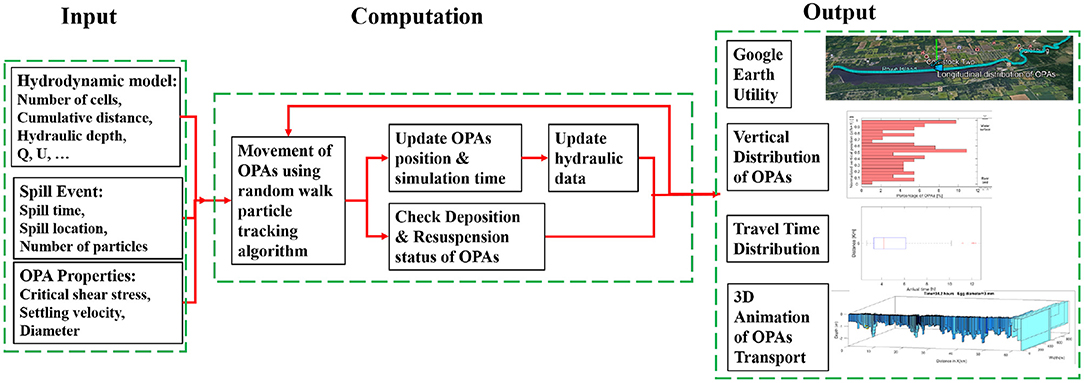
Figure 1. Structure of the FluOil model. Output can be visualized by functionalities in FluOil as well as Google Earth (Google Keyhole, Inc., 2021).
2.1. Random Walk Particle Tracking Algorithm
The transport of OPAs in the water column includes the advection, diffusion, deposition, and resuspension processes. These processes can be represented by the advection-diffusion partial differential equation with source and sink terms accounting for resuspension and deposition in the Eulerian approach (e.g., Hayter et al., 2015). Alternatively, the Lagrangian approach can be applied from the perspective of individual OPA particles. The advection-diffusion equation can be interpreted as a Fokker-Planck equation and solved with a system of stochastic differential equations (SDEs). Then the SDEs can be approximated numerically with discretization schemes, which is the fundamental theory of the random walk particle tracking algorithm (Visser, 1997).
A number of individual particles representing OPAs are used in the random walk particle-tracking algorithm, and the distribution of the particles represents the mass concentration distribution of OPAs in the waterway. The SDEs are discretized in three dimensions to describe the transport of OPAs in the longitudinal, lateral, and vertical directions shown below, respectively.
where Xt, Yt, Zt and Xt+Δt, Yt+Δt, Zt+Δt are coordinates of a particle's position at time t and t+Δt, respectively; Δt is the computational time step; (u, v, w) are velocities in the longitudinal, lateral, and vertical directions, (X, Y, Z), respectively; r is a random number from a normal distribution where the mean is zero and standard deviation is 1; KH and KV are turbulent diffusion coefficients in the horizontal and vertical directions, respectively; and are particle settling velocity, Ws, at t and t+Δt, respectively. The same KH is applied to the random walk scheme in the horizontal (i.e., longitudinal and lateral) directions, whereas in the vertical direction the Visser's (1997) method is adopted to account for the effects of vertical variations of KV. The algorithm has been successfully used in Garcia et al. (2013) and Wang et al. (2020).
Equations for calculating KH and KV are provided by Fischer et al. (1979) and van Rijn (1984):
where h is water depth, is the shear velocity, τb is the channel bed shear stress, and ρw is the density of water. In FluOil model simulation, the calculation of u* is processed when importing the hydraulic data (explained below). β is a coefficient describing the relation between the diffusivity of OPAs and that of the fluid. β is often assumed to be 1 but it can also be computed as a function of the ratio of settling velocity to shear velocity (van Rijn, 1984):
νT is the turbulent/eddy diffusivity (assumed to equal the eddy viscosity) in the vertical direction. There are three commonly used vertical profiles of fluid eddy viscosity: constant (i.e., depth-averaged) (Equation 7), parabolic (Equation 8), and parabolic constant (Equation 9) (Fischer et al., 1979; van Rijn, 1984).
where κ = 0.41 is the von Karman constant. In practice, the parabolic-constant profile is often found to outperform the other two vertical profiles (Garcia et al., 2013; Wang et al., 2020).
Reflective boundary conditions (same as Garcia et al., 2013; Kirca et al., 2016; Laurent et al., 2020) are set to the water surface and channel banks. The boundary condition for the channel bed is set as reflective/depositional/resuspended depending on whether or not the channel bed shear stress exceeds the critical shear stress for OPA deposition/resuspension. The relation between the bed shear and critical shear stresses is checked at each computational time step. If the bed shear stress becomes greater than the critical shear stress, the reflective boundary is in effect. Conversely, if the bed shear stress becomes less than or equal to the critical shear stress, OPA is set to deposit on the bed. For those deposited OPAs, if the bed shear stress becomes greater than the critical shear stress at any time step, the OPA is resuspended and an upward entrainment velocity is assumed, for simplicity, to equal to the settling velocity Ws, thus the distance from the bed after one time step is calculated as WsΔt. It is worth noting that many previous studies only consider steady flow conditions and particles are released initially only in the waterbody. Therefore, entrainment of deposited particles on bed is not needed, since the relation between bed shear stress and critical shear stress does not vary (i.e., bed shear stress > or < = critical shear stress throughout the simulation) thus particles either deposit or not (e.g., Oh et al., 2015; Wang et al., 2020). If particles do not deposit, reflected boundary condition is applied. In some other studies, deposition is neglected even for particles that would deposit, then reflected boundary condition is applied regardless (e.g., Kirca et al., 2016).
2.2. Input Data
2.2.1. Hydraulic Data
There are two ways of inputting hydraulic data into FluOil, one for steady-flow conditions and the other for unsteady-flow conditions. For steady-flow conditions, an Excel table containing columns of computational grid ID, cumulative distance, water depth, flow rate, flow velocity, shear velocity, channel width, and water temperature for each computational grid should be prepared. A template file is provided via Zhu et al. (2022). The steady-flow data can be prepared rapidly with approximated flow characteristics. This option is particularly useful in the early stages of a spill response. When modeling is used to validate historic data, unsteady-flow hydraulic data are preferred.
FluOil imports unsteady-flow data automatically by reading the project file of a one-dimensional HEC-RAS model (Hydrologic Engineering Center, 2021). Its outputs include flow time series of velocity, water depth, channel width, reach length to the downstream cross-section, weighted Manning's roughness coefficient for the main channel, hydraulic radius in the channel, and other variables. FluOil uses the HEC-RAS Controller to process the hydraulic data (Goodell, 2014).
One limitation of one-dimensional hydraulic models for application with FluOil is that only the cross-sectional averaged velocity can be provided. Flow velocities in lateral and vertical directions are neglected (i.e., v = w = 0). However, the longitudinal velocity (u) varies in the vertical and transverse directions, which is critical for calculating the transport of particles. In order to better represent the distribution of longitudinal velocity, instead of using uniform longitudinal velocity for the whole cross section, velocity profile corrections are adopted from Garcia et al. (2015) and applied in transverse and vertical directions. For the transverse direction, the lateral velocity profile proposed by Seo and Baek (2004) is applied. For the vertical direction, the well-known log-law under smooth and rough bottom conditions, respectively, is used (Garcia et al., 2015).
For smooth bottom boundary (e.g., beds covered by mud, silt, or fine sand),
where z is the depth variable measured upward from the datum and ν is the viscosity of water.
For rough bottom boundary (e.g., beds covered by coarse sand or gravel),
where ks is the characteristic roughness height and is estimated using the following relation:
where e stands for the exponent and U is the depth-averaged longitudinal velocity.
2.2.2. OPA Transport Properties
Settling velocity and critical bed shear stress for resuspension are the most important transport properties of OPAs for the FluOil model. The settling velocity is important for OPA transport in suspension vertically, and the critical shear stress for evaluating if OPAs on the stream or lake bed would remain deposited or become resuspended. However, estimating these properties after an oil spill is not easy because the formation of OPAs vary with the type of the spilled oil, the environmental conditions, and how the OPAs form (Gong et al., 2014; Gustitus and Clement, 2017). Therefore, it is ideal to obtain these properties from experimental measurement. For example, settling velocity can be measured for the OPAs formed in laboratory experiments using a settling column and a digital camera (e.g., Waterman and Garcia, 2015). In reality, measurement is not always available, so the following descriptions summarize basic information to assist in estimations.
2.3. Settling Velocity
The settling velocity of an OPA particle mainly depends on its size and density. The shape and makeup of OPAs can take multiple forms (Stoffyn-Egli and Lee, 2002; Fitzpatrick et al., 2015a). Common forms of OPAs involve a spherical oil droplet surrounded by particles or multiple spherical droplets in a particle aggregate (single and multiple droplet aggregate). The size of the spherical-type OPAs can vary from less than 1 μm to tens of μm. Two other aggregate types are also found in laboratory experiments: large, elongated oil masses with internal particles that have various shapes with sizes of tens of μm and can reach 200-300 μm, and thin membranes of clay aggregates that incorporate oil and can attain several mm in length (Stoffyn-Egli and Lee, 2002).
The density of OPAs is another key factor to settling velocity. For all aggregate types, the combination of oil and particles can result in a range of densities so that OPAs can be floating, neutrally buoyant, or negatively buoyant. The negatively buoyant OPAs are focused in FluOil because this OPA particle is able to be deposited. Unlike sediment particles, the density of OPAs can vary appreciably with the oil density, particle density, and the oil/particle volume ratio. The terminal settling velocity for a spherical particle in still water can be estimated by the Stokes law as
where g is the acceleration of gravity, R = (ρs−ρw)/ρw is the submerged specific gravity of the particle, ρs is the density of the particle, ρw is the density of water and D is the diameter of the spherical particle.
A number of empirical relations have been developed to estimate the terminal settling velocity of nonspherical particles. One widely used relation was developed by Dietrich (1982):
where b1 = 2.891394, b2 = 0.95296, b3 = 0.056835, b4 = 0.002892, b5 = 0.000245, and is the particle Reynolds number.
Note that the above relations are for single particles, but the settling velocities of flocs are different because they are affected by the concentration of suspended flocs. A comprehensive review of existing empirical relations for estimating their settling velocities can be found in Garcia (2008).
2.4. Critical Shear Stress
Similar to settling velocity, data on the critical shear stress for resuspension of OPAs is also limited. By analogy with sediment particles, the critical shear stress, τc, might be estimated by the Shields dimensionless parameter, , represented as
For fine-grained sediment (silt and finer), a useful relation to estimate was proposed by Garćıa-Flores and Maza-Alvarez (1997), fitting the Yalin and Karahan diagram (Yalin and Karahan, 1979):
where is the dimensionless particle diameter in the Shields diagram. More details about the explanation of the three ranges of the Shields parameter can be found in Garcia (2008).
Lacking measurement information of D and ρs when estimating for τc may impact the accuracy of OPAs' transport estimations. In this case, the diagram proposed in Wang et al. (2020) may be useful as a guide to choose the rational range of τc for the OPAs, given the density of oil and the size ratio between oil droplets and particles are known.
2.5. GUI and Outputs
The GUI of FluOil (Figure 2) is composed of a menu bar and five main sections including (1) river input data, (2) spill event information, (3) OPA characteristics or properties, (4) simulation setup, and (5) run simulation. Spill event data and OPA properties can be entered through the GUI. In addition, FluOil also can execute batch input where different spill event data and/or OPA properties can be specified in an Excel (Microsoft, Inc., 2021) table. Within the river input data section, two drop-down menus are available to select the option of vertical eddy diffusivity (corresponding to Equations 7-9) and the vertical profile of longitudinal velocity (corresponding to Equations 10 and 11), respectively.
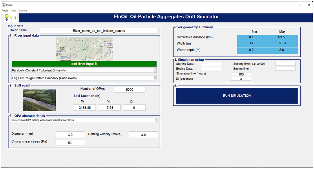
Figure 2. Example of the FluOil graphical user interface (GUI).
When “Load river input file” button is selected, a new window will pop up as shown in Figure 3. As explained previously, two options of inputting hydraulic data are available: steady hydraulics through “River input file” or unsteady hydraulics through “Import HEC-RAS.” An example after inputting a HEC-RAS project file (.prj) is illustrated in Figure 3. The GUI can display the time series of flow and water depth at all cross sections in the HEC-RAS model. When all input data are ready, one can select “Run Simulation” button in the main window (Figure 2). After the simulation is finished, the “Run Simulation” button will automatically change to be “Analyze Results” button.

Figure 3. Example of the FluOil GUI for importing hydraulic data from the unsteady one-dimensional Kalamazoo River HEC-RAS model.
FluOil has utilities to assist users in analyzing and visualizing the spatiotemporally varying OPA profiles, including longitudinal and vertical distribution of suspended or deposited OPAs at any given time, OPA travel time to specified location, and three-dimensional animation of OPA transport. Another useful utility is the projection of modeled results with the Google EarthTM so one can visualize the distribution of suspended and deposited OPAs in relation to the riverine communities (see the Output section in Figure 1).
3. Case Study: Kalamazoo River Oil Spill
The usability of FluOil is demonstrated here by a case study of the 2010 Enbridge Line 6B Kalamazoo River oil spill. This spill event was chosen due to the availability of data that could be used to interpret for setting up the OPA transport scenario. In addition to the efforts on removing oil using conventional methods during the initial phases of the response, the on-site Federal On Scene Coordinator (FOSC) established a Science-Based Support Section to conduct scientific initiatives, in order to understand the distribution and characteristics of the remaining submerged oil, and to provide information to the operations on which to base ongoing response actions (U.S. Environmental Protection Agency, 2016).
The spill was caused by a pipeline rupture on July 26, 2010, which resulted in one of the largest spills of heavy crude oils into an inland waterway in the history of the USA. Over one million gallons of diluted bitumen were spilled into Talmadge Creek, a tributary of the Kalamazoo River near Marshall, Michigan (Figure 4). Spilled diluted bitumen traveled through wetlands and riparian vegetation before entering Kalamazoo River, and passed through approximately 61 km of natural, low-gradient reaches before entering Morrow Lake. Although most of the visible floating oil and residues were collected and removed within 4 months, continuous emergence of oil sheen and tar globs indicated there were submerged oil slicks or oiled sediment on the river bed. It took more than 4 years to clean up the remaining oiled sediment on the river and lake bed. Cleanup efforts were conducted in a reach of the Kalamazoo River from the mouth of Talmadge Creek near Marshall to Morrow Lake near Kalamazoo, approximately 61 km downstream (Fitzpatrick et al., 2015b). Locating the deposited oils was one of the major challenges in the cleanup efforts.
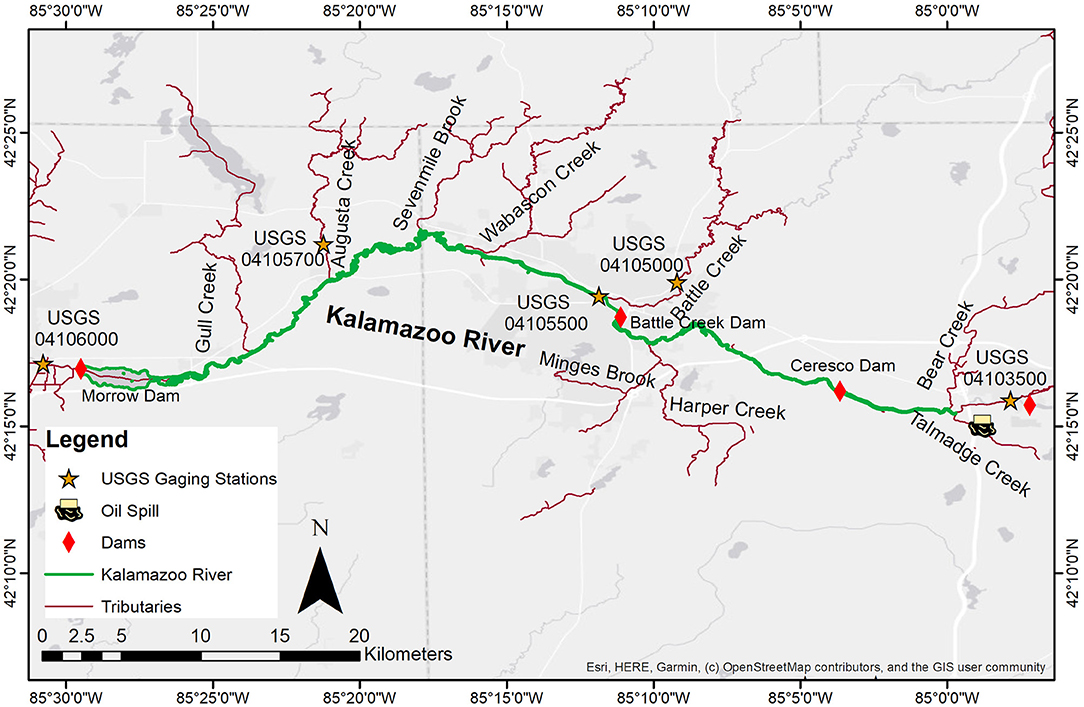
Figure 4. The Kalamazoo River study domain, tributaries, and U.S. Geological Survey gaging stations.
3.1. HEC-RAS Hydrodynamic Model
The Kalamazoo River is a low-gradient meandering river with occasional dams, that is representative of medium-sized rivers across the mid-continent and eastern United States. The hydraulic input data for the FluOil model were generated from a one-dimensional unsteady hydrodynamic model of the Kalamazoo River from the U.S. Geological Survey (USGS) gaging station 04103500 (Kalamazoo River at Marshall, Michigan) to the Morrow Dam using HEC-RAS 5.0.3 (Hydrologic Engineering Center, 2021). Channel geometries were obtained from a steady-flow model previously developed by USGS and AECOM (Hoard et al., 2010). Channel cross sections below the water surface were developed from field surveys conducted in August 2010, whereas light detection and ranging (lidar) data with horizontal resolution of 3 meters were used to provide digital elevation data for the portions of the cross sections that were above the water surface. The river is wide (width/depth ratio of 40 approximately) and has an average gradient of 0.06 percent in the spill-affected 61-km long reach defined earlier. River hydraulics from July 21 to October 31, 2010, a period from just prior of the spill to about 3 months later was simulated for the analysis. The model was calibrated with water surface elevation and discharge data from USGS gaging stations 04103500 and 04105500 (U.S. Geological Survey, 2020) by adjusting Manning's roughness coefficients.
The downstream end of study domain is the Morrow Lake, an impoundment of the Kalamazoo River formed by Morrow Dam. A rating curve was developed for the Morrow Dam (Zhu, 2015) using measured water surface elevation at the headwater of the dam and measured flow discharge at USGS gaging station 04106000 (Figure 4), which was used as downstream boundary condition for the HEC-RAS model.
Taking account for all lateral inflows from tributaries is important for the accuracy of the longitudinal hydraulics of the Kalamazoo River. Eight tributaries were included in the analysis: Talmadge, Bear, Minges Brook-Harper, Battle, Wabascon, Augusta, Gull Creeks, and Sevenmile Brook (Figure 4). Besides the eight tributaries, there are also small watersheds in the study reach and their total drainage areas are not negligible (see Table 1). Data from USGS gaging stations were used to provide inflow boundary conditions (Reneau et al., 2015). Among these tributaries, Battle Creek and Augusta Creek have USGS discharge records, whereas the remaining six tributaries are ungaged thus the discharges needed to be estimated.
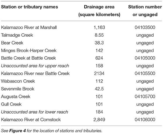
Table 1. Drainage areas of main tributaries and USGS gaging stations.
The Flow Anywhere method (Linhart et al., 2012), a modified drainage-area ratio based method, was used for the estimations. Application of this method represents a regional approach to determine an optimal equation using the regional information contained in each discharge record selected. This method also determines the best reference streamgage from which to transfer same-day discharge information to an ungaged location. The following regression equation is utilized in the method:
where Qu is the discharge at the ungaged location, Au is the drainage area at the ungaged location, QI is the discharge at the index streamgage, AI is the drainage area at the index streamgage, C is a constant, α is the drainage-area-ratio exponent, and γ is the reference streamgage exponent. Using records from eight USGS gaging stations in the vicinity [USGS gaging station IDs 04103500, 04105000, 04105500, 04105700, 04104945, 04106400, 04096405, and 04117500 (U.S. Geological Survey, 2020)] for the regression analysis, we found station 04105500 was the best index streamgage. The three coefficients are C = 0.5102, α = 1.117, and γ = 1.107. Table 1 summarizes the tributaries and USGS gaging stations used in this study.
3.2. OPA Properties
The properties of OPAs in the Kalamazoo River were studied using laboratory experiments by Waterman and Garcia (2015). The most common OPA types were found to be single and multiple droplet aggregates where the OPA volume was dominated by the oil droplet(s) with modest coatings of particles. With predominant sizes ranging from 0.1 to 1 mm, the settling velocity of OPAs was found to be in the range between 1.1 and 11.2 mm/s with the majority in the range between 1.1 and 3.0 mm/s. The critical bed shear stress for resuspension was found to be in the range from 0.0057 to 0.14 Pa. Both settling velocity and critical shear stress can be expected to be highly variable, even more so than the limited laboratory data suggests (Fitzpatrick et al., 2015a). Therefore, four values of critical shear stress (0.01, 0.1, 0.3, and 0.5 Pa) and four values of settling velocity (1, 5, 10, and 20 mm/s) were selected to illustrate the effects of variations in settling velocity and critical shear stress (see Table 2).
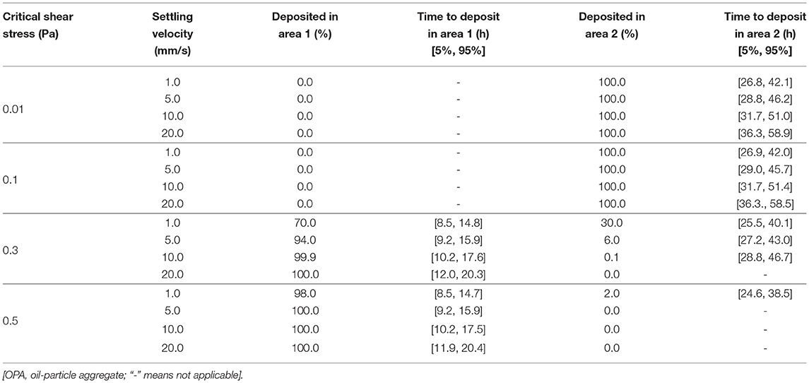
Table 2. Distribution of deposited OPAs and time to deposition.
3.3. Other Setup
Because the spill location was on Talmadge Creek, we used the confluence of the Talmadge Creek with the Kalamazoo River as the starting location of OPAs. The spill time was set at 6 p.m. on July 25, 2010. Five-thousand particles were used in each simulation with a 3 s computational time step. The parabolic constant was used for the vertical profile of turbulent diffusivity, and log-law rough bottom boundary was selected for the vertical profile of longitudinal velocity.
4. Results and Discussion
4.1. Performance of Hydrodynamic Model
Nash-Sutcliffe efficiency (NSE), percent bias (PBIAS), and ratio of the root mean square error to the standard deviation of measured data (RSR) (Moriasi et al., 2007) were computed for evaluating model performance. Simulated water surface elevations and flow discharge with the Kalamazoo River model at the two gaging stations where measurement data are available produced NSE from 0.96 to 0.98, PBIAS from -1.9 to 0, and RSR from 0.14 to 0.19 (see Figure 5). According to the general performance evaluation criteria proposed by Moriasi et al. (2007), a hydrologic model is in the “very good” category if NSE is in the range from 0.75 to 1, PBIAS (%) is ≤ ±10, and RSR is in the range from 0 to 0.5.
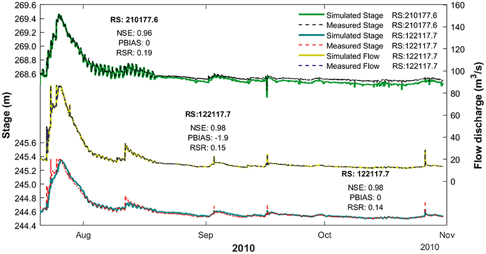
Figure 5. Comparison between measured and simulated water surface elevation at U.S. Geological Survey (USGS) gaging station 04103500 Kalamazoo River at Marshall, Michigan [top, River Station (RS) 210177.6] and USGS gaging station 04105500 Kalamazoo River near Battle Creek, Michigan (bottom, RS 122117.7) (U.S. Geological Survey, 2020). The datum is in NAVD 88. Comparison between measured and simulated flow discharge at USGS gaging station 04105500 Kalamazoo River near Battle Creek, Michigan (middle, RS 122117.7) (U.S. Geological Survey, 2020). NSE, Nash-Sutcliffe efficiency; PBIAS, percent bias; RSR, ratio of the root-mean-square error to the standard deviation of measured data.
4.2. Main Depositional Areas of OPAs
The oil spill occurred during a flood event from July 25 through the first week of August (see Figure 5). Average hydraulic characteristics during this period had a mean velocity of about 1.1 m/s and mean depth of 1.2 m near the USGS streamgage at Marshall, Michigan (04103500). The floodplain of the Kalamazoo River has abundant wetlands, thus suspended and bottom sediments probably have relatively high organic matter content. Based on later measurements of suspended sediment at the Marshall streamgage (Reneau et al., 2015), it can be inferred that, at the time of the spill, the river had relatively (compared to other periods) low suspended sediment concentrations (less than 100 mg/L), with suspended particle sizes mainly in the silt-sized range (65–75%). Water temperature was in the range of 23–25 °C. Assuming that the fraction of spilled oil not recovered by conventional techniques was lost to submergence beneath the water surface, the bitumen that submerged in the Kalamazoo River was greater than 300,000 liters, which is around 10 percent of the total volume of spilled oil (Fitzpatrick et al., 2015a).
There are three main impoundments, upstream of the Ceresco (removed in 2013–2014), Battle Creek, and Morrow dams, which have extensive sediment depositional areas (U.S. Environmental Protection Agency, 2016). Because this oil spill event occurred during a flood event, bed shear stresses in main channels were mostly at high levels (>0.5 Pa) during the simulation period, as shown in Figure 6. Only two large depositional areas are present in the study domain where bed shear stresses were consistently lower than 0.5 Pa: one is the upstream area (area 1 shown in Figure 6B) of the Battle Creek dam [at about 25-km downstream from USGS gaging station 04103500, referred to as the Battle Creek impoundment (U.S. Environmental Protection Agency, 2016)] and the other area (area 2 shown in Figure 6B) is Morrow Lake formed by the Morrow dam at downstream end of the study domain (Zhu et al., 2018). These depositional areas of OPAs agree with submerged oil poling assessments carried out in spring 2011. Samples that were collected within the affected area were categorized into four classifications: none, light, moderate, and heavy. Both Battle Creek and Morrow Lake impoundments were categorized as heavy submerged oil areas (U.S. Environmental Protection Agency, 2016).
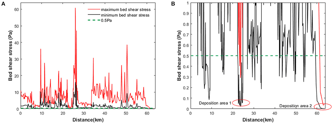
Figure 6. (A) Maximum and minimum bed shear stress simulated by the HEC-RAS Kalamazoo River model at all cross sections in the study domain. (B) A close-up of the bed shear stresses in (A) for the range from 0 to 1 Pa. The green dashed line illustrates one of the critical shear stresses for oil-particle aggregates (OPA) analyzed in the study. The two red circles highlight two dominant potential areas for OPAs to deposit, which are approximately 20 kilometers and 60 kilometers downstream from the starting site, respectively.
4.3. Impacts of Critical Shear Stress and Settling Velocity
The critical shear stress for resuspension, τc, determines whether or not an OPA particle would be deposited at a specific time and location. Considering the uncertainty of this parameter, four values between 0.01 and 0.5 Pa were tested in the model. These values represent a wide coverage of OPAs observed in laboratory experiments (Waterman and Garcia, 2015). Table 2 summarizes the distribution of deposited OPAs and time to deposition under different critical shear stress and settling velocity. When the critical shear stress (τc) was as low as 0.01–0.1 Pa, all OPAs were deposited within area 2 (i.e., Morrow Lake), regardless of settling velocity. As τc increased to 0.3 Pa, some significant amount (70–100%) of OPAs began to deposit in the Battle Creek impoundment (area 1, see Figure 6). When τc reached to 0.5 Pa, almost all OPAs except some with Ws = 1 mm/s, were deposited in the Battle Creek impoundment.
When τc= 0.3 Pa, the distribution of deposited OPAs in those two areas depended on the settling velocity (Ws). With Ws= 1.0 mm/s approximately 70% of the OPAs would deposit in the Battle Creek impoundment and 30% could reach Morrow Lake. While when Ws= 20 mm/s, almost all OPAs could have deposited in Battle Creek impoundment and none would reach Morrow Lake Dam. OPAs with smaller settling velocity generally can transport greater distances. Note that 10 mm/s and 20 mm/s correspond to the settling velocity of very fine and fine sand particles, respectively, which are probably too high for OPAs, although the settling velocity of OPAs could be as large as 30 mm/s depending on oil density, oil droplet size, and sediment size (Wang et al., 2020).
Settling velocity also impacts the time for OPAs to reach the depositional areas. The time for 5 and 95% of the OPAs to deposit in the two depositional areas are given in Table 2. For a given critical shear stress, OPAs with smaller settling velocity reached the deposition areas faster. For example, when τc= 0.01 Pa, the 5% mass of OPAs that settled in the Morrow Lake deposition area took 26.8 and 36.3 h for Ws= 1 and 20 mm/s, respectively, with a difference of 9.5 h. This difference increased to 16.8 h for the 95% mass of OPAs. Understanding and quantifying those variations are important for oil spill response.
Similar to sediment particles or other negatively buoyant particles, the concentrations of OPAs generally increase in the direction from water surface to channel bed in the water column. This result is known as the Rouse concentration profile for suspended sediment (Garcia, 2008). As the water generally flows faster near the surface and slower near the bottom (see Equations 10 and 11), if more OPAs appear in the lower water column, they will subject to lower transport velocity than those stay in the upper water column. With a lower settling velocity, the travel distance of the OPAs for a given time increases substantially (see Figure 7). The difference in travel distance increases with time. At 5 h after the oil spill, OPAs with Ws= 20 mm/s traveled up to 11 km downstream, whereas OPAs with Ws= 1 mm/s travel up to 17 km downstream. At 15 h, OPAs with Ws= 20 mm/s traveled up to 30 km downstream, while OPAs with Ws= 1 mm/s can reach up to 45 km downstream.
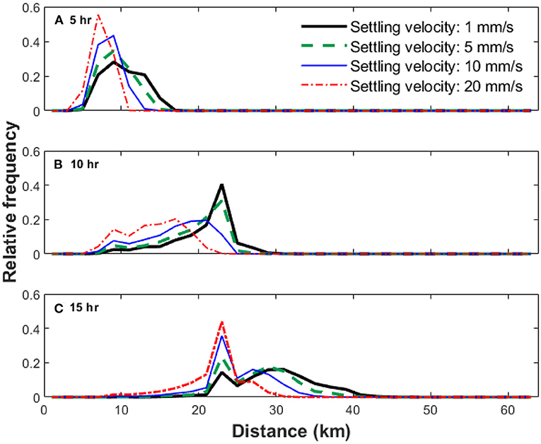
Figure 7. Longitudinal distribution of suspended oil-particle aggregates (OPA) under critical shear stress of 0.1 Pa and four settling velocities; 1, 5, 10, and 20 mm/s. Results at the end of: (A) 5 h, (B) 10 h, and (C) 15 h after the oil spill. The resolution of the plots is 2 km.
4.4. Limitations
There are some limitations of the FluOil model and its application to the Kalamazoo River oil spill. First, it imports only a one-dimensional HEC-RAS hydraulic model for unsteady-flow conditions, whereas two- or even three-dimensional hydrodynamics are sometimes necessary to identify small depositional areas such as bank margins, cutoff channels and meanders (Zhu, 2015) and three-dimensional hydrodynamics are almost necessary for resolving lake environments (Zhu et al., 2018). Deposition of OPAs occurred along channel margins, backwaters, side channels, and oxbows, and in impoundments throughout the entire 61-km stretch of the river affected by the oil spill. Also, deposition and resuspension on river banks are neglected as our understanding about the thresholds for the fate of OPAs on the river banks (i.e., critical shear stresses for deposition and resuspension) is limited. The random walk particle tracking algorithm can handle three-dimensional hydrodynamics, but new utilities must be developed to import the hydrodynamic data into the model. The utilities for analyzing the hydrodynamic data should also be updated to accompany the three-dimensional modeling results.
FluOil operates under the assumptions that (1) OPAs have been formed previously and are in the water column within the modeled reach, and (2) OPA properties do not change during the transport. These assumptions may not always be valid. Zhao et al. (2016) proposed a model for simulating the formation of single-droplet-type OPAs. The model was successfully adopted by Jones and Garcia (2018) and Wang et al. (2020) to investigate the effects of the formation process on the fate and transport of OPAs. This OPA formation model could be implemented into FluOil to expand its applicability. There are situations where OPAs are formed by particles acting as projectiles penetrating the oil droplets. The formed OPAs could disintegrate over time due to the protrusion of particles from the oil droplet (Zhao et al., 2017).
In the experiments conducted by Waterman and Garcia (2015), OPAs were obtained by replicating solid- and droplet-type OPAs using oil from Enbridge and river sediment from the Kalamazoo River in the laboratory, not OPAs from the river. Therefore, the range of settling velocity and critical bed shear stress based on the experiments may not reflect the range of OPAs in the river. For example, OPAs can consist of organic matter that does exist in the Kalamazoo River. Since organic matter is generally lighter than sediment particles, Organic matter dominated OPAs might have smaller settling velocities thus longer traveling distance before settling. Additional research for determining the range of settling velocities and critical shear stresses resulting from different types of oils and sediments would increase understanding of OPAs' transport properties.
To authors best knowledge, modeling particle re-entrainment/resuspension has not been studied sufficiently for Random Walk Particle Tracking approaches, as sediment particle resuspension is a complex phenomenon (Cameron et al., 2020), regardless of OPAs that have more varying characteristics than sediment particles. Therefore, it is assumed that re-entrainment velocity is equal to the settling velocity for simplicity. This simplification is not sensitive to the overall results, particularly for particle clouds. The primary role of the re-entrainment velocity is to provide an initial displacement distance above the bed. After that time step (normally each time step is several seconds), particle motion in the vertical direction will be calculated by Equation (3), which makes the vertical distribution of particles tend to the equilibrium state (i.e., the Rouse profile Garcia, 2008). If hydrodynamics is simulated using direct numerical simulation (DNS) or large eddy simulation (LES) (Soldati and Marchioli, 2012), particle motion can be modeled using force balance equations instead of random walk particle tracking (e.g., Chang and Scotti, 2006). The force balance equations are used to solve for particle velocities, then particle position can be calculated from the velocities. However, even for this approach (i.e., DNS/LES + Particle Tracking using force balance equations), treating re-entrainment/resuspension rate is a challenge (Soldati and Marchioli, 2012). The DNS/LES approach is not applicable for simulating the transport of OPAs in rivers because it is very computationally expensive.
5. Conclusion
The FluOil model is a novel, open-source software for modeling the transport of oil-particle aggregates (OPAs) in inland waterways. The model can automatically import channel geometry and hydraulic data from one-dimensional unsteady hydraulic models using the Hydrologic Engineering Center's River Analysis System (HEC-RAS), a public domain software widely used for simulating river hydraulics for flood studies or river engineering studies. FluOil simulates the advection, diffusion, deposition, and resuspension of OPAs by implementing the random walk particle tracking algorithm. The usability of FluOil is demonstrated with the application to the 2010 Kalamazoo River oil spill case study. FluOil is used to analyze the effects of two of the most important OPA properties, settling velocity and critical shear stress for resuspension, on the transport and OPA deposition after the oil spill. Settling velocity determines the distribution of OPAs in the vertical direction and thus the travel velocity they subject to, whereas critical shear stress determines where and when OPAs are deposited.
Data Availability Statement
Publicly available datasets were analyzed in this study. This data can be found at: Zhu et al. (2022).
Author Contributions
ZZ, DS, and YL contributed to conception and design of the study and wrote the first draft of the manuscript. YL performed the modeling analysis. HK, SW, FF, and MG wrote sections of the manuscript. All authors contributed to manuscript revision and approved the submitted version.
Funding
This research was funded by the 2017 USGS Midwest Region Flex Fund and the U.S. Geological Survey (USGS) Cooperative Ecosystem Studies Unit Program (grant nos. G18AC00023 and G19AC00054).
Conflict of Interest
The authors declare that the research was conducted in the absence of any commercial or financial relationships that could be construed as a potential conflict of interest.
Publisher's Note
All claims expressed in this article are solely those of the authors and do not necessarily represent those of their affiliated organizations, or those of the publisher, the editors and the reviewers. Any product that may be evaluated in this article, or claim that may be made by its manufacturer, is not guaranteed or endorsed by the publisher.
Acknowledgments
We thank Dr. Tatiana Garcia for helpful discussion about the design of the FluOil model. This article has been peer reviewed and approved for publication consistent with U.S. Geological Survey Fundamental Science Practices (https://pubs.usgs.gov/circ/1367/).
References
Amir-Heidari, P., Arneborg, L., Lindgren, J. F., Lindhe, A., Rosén, L., Raie, M., et al. (2019). A state-of-the-art model for spatial and stochastic oil spill risk assessment: a case study of oil spill from a shipwreck. Environ. Int. 126, 309–320. doi: 10.1016/j.envint.2019.02.037
Bandara, U. C., Yapa, P. D., and Xie, H. (2011). Fate and transport of oil in sediment laden marine waters. J. Hydroenviron. Res. 5, 145–156. doi: 10.1016/j.jher.2011.03.002
Barron, M. G., Vivian, D. N., Heintz, R. A., and Yim, U. H. (2020). Long-term ecological impacts from oil spills: comparison of exxon valdez, hebei spirit, and deepwater horizon. Environ. Sci. Technol. 54, 6456–6467. doi: 10.1021/acs.est.9b05020
Boufadel, M. C., Fitzpatrick, F., Cui, F., and Lee, K. (2019). Computation of the mixing energy in rivers for oil dispersion. J. Environ. Eng. 145, 06019005. doi: 10.1061/(ASCE)EE.1943-7870.0001581
Brody, T. M., Bianca, P. D., and Krysa, J. (2012). Analysis of inland crude oil spill threats, vulnerabilities, and emergency response in the midwest united states. Risk Anal. 32, 1741–1749. doi: 10.1111/j.1539-6924.2012.01813.x
Cameron, S. M., Nikora, V. I., and Witz, M. J. (2020). Entrainment of sediment particles by very large-scale motions. J. Fluid Mech. 888:A7. doi: 10.1017/jfm.2020.24
Chang, Y. S., and Scotti, A. (2006). Turbulent convection of suspended sediments due to flow reversal. J. Geophys. Res. 111, C07001. doi: 10.1029/2005JC003240
Dietrich, W. E. (1982). Settling velocity of natural particles. Water Resour. Res. 18, 1615–1626. doi: 10.1029/WR018i006p01615
Fischer, H., List, E., Koh, R., Imberger, J., and Brooks, N. (1979). Mixing in Inland and Coastal Waters. New York, NY: Academic Press.
Fitzpatrick, F. A., Boufadel, M. C., Johnson, R., Lee, K. W., Graan, T. P., Bejarano, A. C., et al. (2015a). Oil-Particle Interactions and Submergence from Crude Oil Spills in Marine and Freshwater Environments? review of the Science and Future Science Needs. Technical Report, U.S. Geological Survey Open-File Report 2015–1076.
Fitzpatrick, F. A., Johnson, R., Zhu, Z., Waterman, D., Mcculloch, R. D., Hayter, E. J., et al. (2015b). “Integrated modeling approach for fate and transport of submerged oil an oil-particle aggregates in a freshwater riverine environment,” in Proceedings for the 2015 Joint Federal Interagency Conference on Sedimentation and Hydrologic Modeling (SEDHYD 2015) (Reno, NV), 1783–1794.
Garcia, M. (Ed.). (2008). Sedimentation Engineering: Processes, Measurements, Modeling, and Practice. Reston, VA: American Society of Civil Engineers.
Garcia, T., Jackson, P. R., Murphy, E. A., Valocchi, A. J., and Garcia, M. H. (2013). Development of a fluvial egg drift simulator to evaluate the transport and dispersion of asian carp eggs in rivers. Ecol. Modell. 263, 211–222. doi: 10.1016/j.ecolmodel.2013.05.005
Garcia, T., Murphy, E. A., Jackson, P. R., and Garcia, M. H. (2015). Application of the FluEgg model to predict transport of Asian carp eggs in the Saint Joseph River (Great Lakes tributary). J. Great Lakes Res. 41, 374–386. doi: 10.1016/j.jglr.2015.02.003
García-Flores, M., and Maza-Alvarez, J. (1997). Inicio de movimiento y acorazamiento. capítulo 8 del manual de ingeniería de ríos. Series Del Instituto fr Ingeniería, 592.
Gong, Y., Zhao, X., Cai, Z., O'Reilly, S., Hao, X., and Zhao, D. (2014). A review of oil, dispersed oil and sediment interactions in the aquatic environment: influence on the fate, transport and remediation of oil spills. Mar. Pollut. Bull. 79, 16–33. doi: 10.1016/j.marpolbul.2013.12.024
Goodell, C. R. (2014). Breaking the HEC-RAS Code: A User's Guide to Automating HEC-RAS. h2ls, 1st Edn.
Google Keyhole Inc. (2021). Google Earth program. Available1 online at: https://earth.google.com (accessed February 14, 2022).
Gustitus, S. A., and Clement, T. P. (2017). Formation, fate, and impacts of microscopic and macroscopic oil-sediment residues in nearshore marine environments: a critical review. Rev. Geophys. 55, 1130–1157. doi: 10.1002/2017RG000572
Hayter, E., McCulloch, R., Redder, T., Boufadel, M., Johnson, R., and Fitzpatrick, F. (2015). Modeling the Transport of Oil Particle Aggregates and Mixed Sediment in Surface Waters. Vicksburg, MS: U.S. Army Corps of Engineers Engineer Research and Development Center.
Hoard, C. J., Fowler, K. K., Kim, M. H., Menke, C. D., Morlock, S. E., Peppler, M. C., et al. (2010). Flood-Inundation Maps for a 15-Mile Reach of the Kalamazoo River From Marshall to Battle Creek, Michigan. Reston, VA: U.S. Geological Survey Scientific Investigations Map 3135.
Hydrologic Engineering Center (2021). Hydrologic Engineering Center River Analysis System. Available online at: https://www.hec.usace.army.mil/software/hec-ras/download.aspx (accessed February 14, 2022).
Jones, L., and Garcia, M. H. (2018). Development of a rapid response riverine oil particle aggregate formation, transport, and fate model. J. Environ. Eng. 144, 04018125. doi: 10.1061/(ASCE)EE.1943-7870.0001470
Kirca, V. S. O., Sumer, B. M., Steffensen, M., Jensen, K. L., and Fuhrman, D. R. (2016). Longitudinal dispersion of heavy particles in an oscillating tunnel and application to wave boundary layers. J. Ocean Eng. Mar. Energy 2, 59–83. doi: 10.1007/s40722-015-0039-x
Laurent, C., Querin, S., Solidoro, C., and Canu, D. M. (2020). Modelling marine particle dynamics with LTRANS-Zlev: implementation and validation. Environ. Model. Softw. 125, 104621. doi: 10.1016/j.envsoft.2020.104621
Linhart, S. M., Nania, J. F., and Sanders C. L. Jr, Archfield, S. A. (2012). Computing daily mean streamflow at ungaged locations in iowa by using the flow anywhere and flow duration curve transfer statistical methods. Techincal report, U.S. Geological Survey Scientific Investigations Report 2012–5232.
Microsoft Inc. (2021). Excel Program. Available online at: https://www.microsoft.com/microsoft-365/excel (accessed February 14, 2022).
Moriasi, D., Arnold, J., Van Liew, M., Bingner, R., Harmel, R., and Veith, T. (2007). Model evaluation guidelines for systematic quantification of accuracy in watershed simulations. Trans. ASABE 50, 885–900. doi: 10.13031/2013.23153
Niu, H., Li, Z., Lee, K., Kepkay, P., and Mullin, J. V. (2011). Modelling the transport of oil-mineral-aggregates (OMAs) in the marine environment and assessment of their potential risks. Environ. Model. Assess. 16, 61–75. doi: 10.1007/s10666-010-9228-0
Oh, J., Tsai, C. W., and Choi, S.-U. (2015). Quantifying the uncertainty associated with estimating sediment concentrations in open channel flows using the stochastic particle tracking method. J. Hydraulic Eng. 141, 04015031. doi: 10.1061/(ASCE)HY.1943-7900.0001045
Pando, S., Juliano, M. F., García, R., de Jesus Mendes, P. A., and Thomsen, L. (2013). Application of a lagrangian transport model to organo-mineral aggregates within the Nazaré canyon. Biogeosciences 10, 4103–4115. doi: 10.5194/bg-10-4103-2013
Reneau, P., Soong, D., Hoard, C., and Fitzpatrick, F. (2015). Hydrodynamic-Assessment Data Associated With the July 2010 Line 6B Spill Into the Kalamazoo River, Michigan, 2012-14. Technical Report, U.S. Geological Survey Open-File Report 2015–1205.
Seo, I. W., and Baek, K. O. (2004). Estimation of the longitudinal dispersion coefficient using the velocity profile in natural streams. J. Hydraulic Eng. 130, 227–236. doi: 10.1061/(ASCE)0733-9429(2004)130:3(227)
Soldati, A., and Marchioli, C. (2012). Sediment transport in steady turbulent boundary layers: potentials, limitations, and perspectives for Lagrangian tracking in DNS and LES. Adv. Water Resour. 48, 18–30. doi: 10.1016/j.advwatres.2012.05.011
Stoffyn-Egli, P., and Lee, K. (2002). Formation and characterization of oil-mineral aggregates. Spill Sci. Technol. Bull. 8, 31–44. doi: 10.1016/S.1353-2561(02)00128-7
U. S. Environmental Protection Agency (2016). FOSC Desk Report for the Enbridge Line 6b Oil Spill in Marshall, Michigan. Available online at: https://www.epa.gov/enbridge-spill-michigan/fosc-desk-report-enbridge-oil-spill (accessed February 14, 2022).
U. S. Geological Survey (2020). USGS Water Data for the Nation: U.S. Geological Survey National Water Information System Database, Reston, VA: USGS.
van Rijn, L. (1984). Sediment transport, part ii: suspended load transport. J. Hydraulic Eng. 110, 1613–1641. doi: 10.1061/(ASCE)0733-9429(1984)110:11(1613)
Visser, A. W. (1997). Using random walk models to simulate the vertical distribution of particles in a turbulent water column. Mar. Ecol. Progr. Ser. 158, 275–281. doi: 10.3354/meps158275
Wang, S., Yang, Y., Zhu, Z., Jin, L., and Ou, S. (2020). Riverine deposition pattern of oil particle aggregates considering the coagulation effect. Sci. Total Environ. 739, 140371. doi: 10.1016/j.scitotenv.2020.140371
Waterman, D., and Garcia, M. H. (2015). Laboratory Tests of Oil-Particle Interactions in a Freshwater Riverine Environment with Cold Lake Blend Weathered Bitumen. University of Illinois at Urbana-Champaign, Civil Engineering Studies, Hydraulic Engineering Series No 106.
Yalin, M. S., and Karahan, E. (1979). Inception of sediment transport. J. Hydraulics Division 105, 1433–1443. doi: 10.1061/JYCEAJ.0005306
Yoshioka, G., and Carpenter, M. (2002). “Characteristics of reported inland and coastal oil spills,” in Fourth Biennial Freshwater Spills Symposium (Fairfax, VA).
Zhao, L., Boufadel, M. C., Geng, X., Lee, K., King, T., Robinson, B., et al. (2016). A-DROP: A predictive model for the formation of oil particle aggregates (OPAs). Mar. Pollut. Bull. 106, 245–259. doi: 10.1016/j.marpolbul.2016.02.057
Zhao, L., Boufadel, M. C., Katz, J., Haspel, G., Lee, K., King, T., et al. (2017). A new mechanism of sediment attachment to oil in turbulent flows: projectile particles. Environ. Sci. Technol. 51, 11020–11028. doi: 10.1021/acs.est.7b02032
Zhao, L., Torlapati, J., Boufadel, M. C., King, T., Robinson, B., and Lee, K. (2014). VDROP: a comprehensive model for droplet formation of oils and gases in liquids - Incorporation of the interfacial tension and droplet viscosity. Chem. Eng. J. 253, 93–106. doi: 10.1016/j.cej.2014.04.082
Zhu, Z. (2015). Modeling the transport and fate of oil-particle aggregates after an oil spill in inland waterways (Ph.D. thesis). University of Illinois at Urbana-Champaign.
Zhu, Z., Miles, K. J., and Soong, D. (2022). FluOil Model and Related Datasets for Kalamazoo River, Michigan Oil Spill: July 21 to October 31, 2010. Reston, VA: U.S. Geological Survey data release. doi: 10.5066/P99MJ6MD
Zhu, Z., Waterman, D. M., and Garcia, M. H. (2018). Modeling the transport of oil-particle aggregates resulting from an oil spill in a freshwater environment. Environ. Fluid Mech. 18, 967–984. doi: 10.1007/s10652-018-9581-0
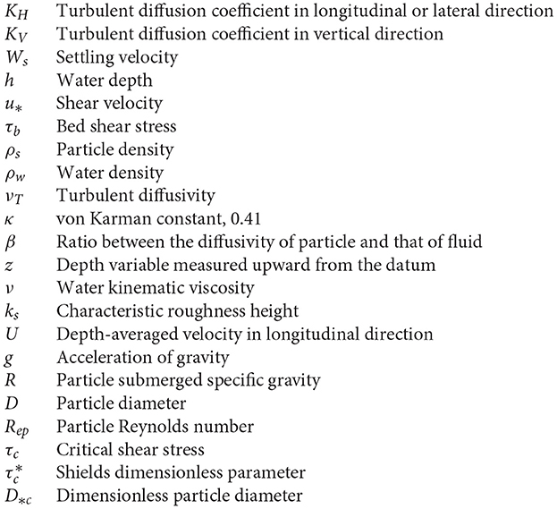
List of Symbols
Keywords: oil spill, oil-particle aggregate, decision support tool, particle tracking, Kalamazoo River, deposition and resuspension
Citation: Li Y, Zhu Z, Soong DT, Khorasani H, Wang S, Fitzpatrick F and Garcia MH (2022) FluOil: A Novel Tool for Modeling the Transport of Oil-Particle Aggregates in Inland Waterways. Front. Water 3:771764. doi: 10.3389/frwa.2021.771764
Received: 07 September 2021; Accepted: 22 November 2021;
Published: 11 March 2022.
Edited by:
Constantinos V. Chrysikopoulos, Technical University of Crete, GreeceReviewed by:
Michel C. Boufadel, New Jersey Institute of Technology, United StatesLinlin Cui, College of William and Mary, United States
Copyright © 2022 Li, Zhu, Soong, Khorasani, Wang, Fitzpatrick and Garcia. This is an open-access article distributed under the terms of the Creative Commons Attribution License (CC BY). The use, distribution or reproduction in other forums is permitted, provided the original author(s) and the copyright owner(s) are credited and that the original publication in this journal is cited, in accordance with accepted academic practice. No use, distribution or reproduction is permitted which does not comply with these terms.
*Correspondence: Zhenduo Zhu, emhlbmR1b3pAYnVmZmFsby5lZHU=; David T. Soong, ZHNvb25nQHVzZ3MuZ292