 Maxime Claprood1*
 Erwan Gloaguen1Thomas Béraud1
 Martin Blouin2Christian Dupuis3Philippe Ferron4
 Michel Ouellet4Michel Chaussé4Richard Martel1Daniel Paradis5Jean-Marc Ballard1
- 1Institut National de la Recherche Scientifique, Eau Terre Environnement Research Centre, Quebec City, QC, Canada
- 2MBMS Solutions, Quebec City, QC, Canada
- 3Geology and Geological Engineering Department, Laval University, Quebec City, QC, Canada
- 4Ministère de l'Environnement et de la Lutte contre les Changements Climatiques, Quebec City, QC, Canada
- 5Geological Survey of Canada, Quebec City, QC, Canada
Building a representative three-dimensional conceptual model of the hydrostratigraphic units is the critical first step when undertaking a hydrogeological assessment. The construction of such conceptual model requires integrating all geological data available for reducing the uncertainty of the conceptual model. In addition, the different types of data collected do not have the same level of uncertainty, and this has to be considered during the modeling. This manuscript presents a geostatistical workflow developed to integrate high resolution seismic reflection data with geological well markers and well logs. The proposed workflow allows reducing and quantifying the uncertainty when developing the conceptual model of hydrostratigraphic units and estimating the spatial distribution of hydraulic conductivity needed to simulate groundwater flow. The study involves the field investigation and numerical modeling for understanding the hydraulic connection between a local sand and gravel esker aquifer overlying a fractured bedrock regional aquifer. Seismic reflection data recorded in 2019 and 2021 significantly modify the conceptual model originally envisioned at site by discovering unknown deep esker extensions. Seismic data also help reducing the spatial uncertainty by delimiting the lateral extents, thickness, and depth of the esker aquifer between existing boreholes. Thickness maps of major hydrostratigraphic units are computed by first interpolating the data with higher uncertainty, which are then locally deformed by successive kriging with external drift to honor data with lower uncertainty. Well logs are then combined with seismic reflection data to better represent the spatial distribution of hydrofacies within the esker aquifer, and identify subunits in the bedrock aquifer. These modifications in the conceptual model of hydrostratigraphic units and the better understanding of the vertical heterogeneity of the hydraulic conductivity significantly impact the simulation of groundwater flow, both regionally and locally at site.
1. Introduction
An important first step to complete during a hydrogeological assessment is the development of a representative conceptual model of groundwater flow. As discussed in Gupta et al. (2012) and summarized in Enemark et al. (2019), building a conceptual model can be divided into five formal stages: (i) conceptual physical structure, (ii) conceptual process structure, (iii) spatial variability structure, (iv) equation structure and (v) computational structure. This manuscript will be focussing on the first stage of the process, more precisely on modeling the spatial distribution of major hydrostratigraphic units and hydrofacies during the hydrogeological conceptualization. As mentioned by Doherty and Welter (2010); Enemark et al. (2019), an inadequate conceptual model will introduced some bias when estimating the hydraulic parameters distribution and will lead to shortcomings during the calibration.
A hydrogeological assessment requires an adequate characterization of the spatial distribution and heterogeneity of major hydrofacies, in other words lithologies having stationary and specific values of hydraulic conductivity. The scale of the characterization of this heterogeneity is case dependent, and should allow building numerical models of hydraulic conductivity used to manage the aquifer. Building a numerical model of groundwater flow involves integrating data coming from multiple sources; each dataset having its own precision, resolution, and uncertainty (Rubin and Hubbard, 2005).
Geoscientists are aware of the inherent uncertainty associated with the recording of field data. However, this uncertainty is frequently overlooked for simplicity and financial motivations when developing the conceptual model. The conceptual model may be developed considering the data to be 100% accurate, or by oversimplifying the hypothesis behind its construction. This inconsideration of uncertainty may induce some significant bias when developing the conceptual physical structure during a hydrogeology assessment; by failing to detect some important hydrogeologic features such as incised channels or flow barriers, by generating smoother simulated groundwater flow patterns, or by miscalculating the transport time of contaminant particles (Paradis et al., 2010; Paradis and Lefebvre, 2013).
As mentioned by Enemark et al. (2019), two types of solutions are commonly applied to address the uncertainty in the conceptual model; reducing the uncertainty of a consensus conceptual model by acquiring additional geophysical data of high spatial coverage, or quantifying the impacts of uncertainty on the possible outcomes by generating multiples probable scenarios. While generating multiple probable scenarios is recognized as the optimal approach for considering the uncertainty when developing the conceptual physical model, it is often complex to apply in real case scenarios. For example, Visser and Markov (2019) applied a data fusion technique to explicitly model the observation uncertainty for different sources of data for mapping cover thickness. Geological observation errors are needed to adequately sample all probable scenarios of the conceptual physical model. However, the observation errors on geological data are not estimated in our case. These errors are highly dependent on the source data collected and can vary within a single source of data, making such approach difficult to implement here.
For these reasons, the consensus model scenario is followed in this project, using a nested approach to merge large coverage low quality data at regional scale with low coverage high-quality data at local scale. This nested approach is designed to reduce the uncertainty when building a single conceptual model of the major hydrostratigraphic units and hydrofacies at site, by sequentially integrating the available data.
Due to the limitations of conventional hydraulic characterization to model the spatial variations of hydraulic parameters, hydrogeophysics is increasingly recognized as an effective alternative to better image spatial distribution of hydraulic properties, which requires the translation of indirect geophysical data into hydraulic properties (Day-Lewis et al., 2005; Rubin and Hubbard, 2005). The gain of using geophysical data for hydrogeological characterization relies on the almost continuous spatial coverage of geophysical methods, which may be helpful to infer spatial continuity of heterogeneity of hydraulic conductivity.
Reliable predictions in hydrofacies and hydraulic conductivity from geophysical data should however be based on reliable statistical or physical relations between hydraulic and geophysical data, which are usually subject to a large degree of uncertainty (Chen et al., 2001). The major problem with the integration of hydro-geophysical data is non-uniqueness in the hydro-geophysical relations. Typical causes of non-uniqueness are the scale and the resolution disparity between hydraulic and geophysical measurements, and the uncertainty associated with field data acquisition and interpretation (e.g., noisy measurements, location errors). The motivation of the work is to use large coverage geophysical data (seismic reflection) in conjunction with high resolution hydrogeological data measured along wells to improve the accuracy in representing the geometry and hydraulic parameters of a paleoglacial aquifer.
The site, which exact location can not be disclosed, has been studied over several decades. An initial three-dimensional (3D) conceptual model of hydrostratigraphic units was built using well markers information (Pontlevoy, 2004; Tremblay and Lamothe, 2005) and surficial geology map. This initial conceptual physical model delineates an elongated esker formation as a single and continuous channel comprised of fluvioglacial coarse sand and gravel sediments within a thick sequence of marine clay and till above a fractured bedrock. This conceptual physical model was then used to build a regional and a local groundwater flow models to predict the flow path and capture area around pumping wells. The calibration of this initial groundwater flow model was not satisfactory, and new geological observations were needed to improved our knowledge at site. As new data become available and knowledge at site improved, the initial conceptual model needs to be updated to match these new observations. Areas of high uncertainties were also identified when updating the conceptual physical model; which lead to (i) the acquisition of high resolution seismic reflection data to reduce that uncertainty, and (ii) the drilling of ten boreholes to validate the information derived from seismic reflection data.
Commonly used for oil and gas discovery, seismic reflection is being applied increasingly for environmental and hydrogeology assessment since the 1980's (Rubin and Hubbard, 2005) due to the use of seismic landstreamers. The use of landstreamers is cost effective for near-surface applications and allows recording both P- and S-wave data (Van der Veen et al., 2001; Inazaka, 2004; Pugin et al., 2009). Several studies have used high resolution seismic reflection survey to complete hydrogeological assessments of tunnel valley aquifers (Sharpe et al., 2003; Tremblay et al., 2010; Pugin et al., 2013, 2014), which are similar geological settings than that of the site of study.
The manuscript objectives are two-fold : (i) to present the nested approach used for considering uncertainty when integrating geological data in building the conceptual physical model, and (ii) to demonstrate the importance of acquiring high resolution seismic reflection surface data for reducing the uncertainty when modeling the spatial extents of main hydrostratigraphic units. The methodologies developed for achieving both objectives are described by presenting their application on modeling the thickness of the main esker formation at site, which represents the local aquifer at site. The approach will allow first to better understand the groundwater budget at a regional scale (80 km × 100 km) so as to mimic the regional groundwater flux. The nested approach developed also makes it possible to build a high resolution local scale (2 km × 2 km) numerical model to optimize a system of groundwater catchment.
Ten boreholes were drilled locally to confirm the hydrostratigraphic interpretations from the seismic reflection survey. Well logs were acquired at these boreholes to better characterize the vertical distribution of hydrofacies and hydraulic parameters within each of the major hydrostratigraphic units previously modeled. Geological interpretation from these boreholes will be briefly shown to present the whole conceptual physical model at site.
2. Study Area
The project is located in southern Quebec (Canada), at proximity to the city of Montreal. The area of interest is 9.5 km long by 8.2 km large, for a total area of 78 km2 (Figure 1). The topography of the region is mostly flat, with some rolling drumlin hills, and ranges in elevation from 24 to 64 m above sea level (MASL).
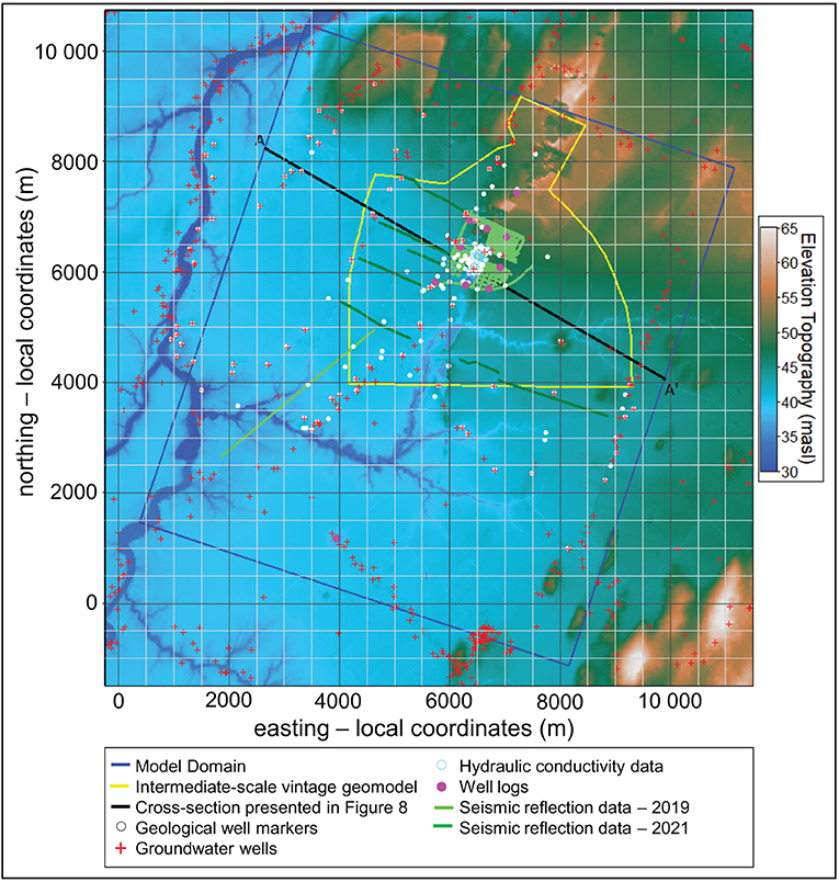
Figure 1. Map of surface topography and available data in the model region.
2.1. Geological Background
The bedrock is composed of Paleozoic sedimentary dolomites and orthoquartzites from the St. Lawrence Lowlands (Globensky, 1986). Its geology and hydrogeological properties are further described by Lavigne et al. (2010), and Lamontagne and Nastev (2010). Depth to bedrock, as recorded from geotechnical investigations and water wells records, ranges from 0 to 50 m. The maximum depth to bedrock within the model is 46 m. The most important hydrostratigraphic units overlying the bedrock are sediments from the Quaternary Period, and are from bottom to top: regional Till unit, glaciofluvial sediments from the Esker Sand and Gravel Unit, and fine grained marine sediments from the Marine Clay unit. Some recent organic sediments and filling materials are present locally in the model domain. The complete Quaternary sequence is described by LaSalle (1981); Dion et al. (1986); Tremblay and Lamothe (2005); Tremblay (2008); Lamontagne and Nastev (2010); Tremblay et al. (2010). The spatial distribution of these units are represented in the surface geology map (Figure 2).
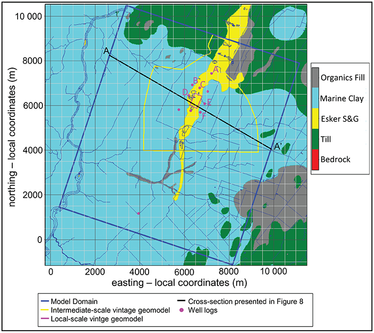
Figure 2. Map of surface geology in the model region.
The Till unit is deposited above the bedrock, and is the main deposits from the glacier. Its thickness varies from absent to 23.5 m within the model region. It is composed of compact moraine unit with a heterogeneous distribution of materials. The Esker Sand and Gravel unit above is a very heterogeneous distribution of material, and is locally present at site, reaching a maximum thickness of 31.5 m. It is comprised of the main esker channels deposited by high energy underground rivers from melting water from glaciers, and lateral silty and clayed sands subunit. The outcropping portion of the esker channels is approximately 10 km long and a few hundred meters wide, trending at a 30° azimuth. The Esker Sand and Gravel unit is modeled as a unique unit in the conceptual model because it is undifferentiated in well markers. Fine grained marine sediments form the thick (maximum thickness of 28.7 m) Marine Clay unit deposited in the Champlain Sea.
2.2. Hydrogeological Background
The hydrogeological system at site is composed of a local high hydraulic conductivity aquifer (the Esker Sand and Gravel unit) isolated by the low hydraulic conductivity sediments of the Marine Clay unit. The Marine Clay unit acts as a major barrier to flow and as a confinement unit above the Esker Sand and Gravel unit, where it is present.
The heterogeneous sand and gravel materials from the esker have high but variable hydraulic conductivity (from 1 × 10⁻⁶ms−1 to 1 × 10⁻³ms−1). The esker is partially isolated from the underlying regional bedrock aquifer by the Till unit with varying thickness. The Till unit is considered as an aquitard where its thickness is larger than 3 m. However, the variability in thickness and hydraulic properties of the Till unit is known to allow some degree of hydraulic connection between the local esker aquifer above and the regional fractured bedrock below. The bedrock aquifer is considered as a regional aquifer, and is extensively used for agriculture, municipal, and industrial applications in the region. Its hydraulic conductivity is also highly variable (from 1 × 10⁻¹⁰ms−1 to 1 × 10⁻⁴ms−1), and depends on the level of fracturing.
3. Data
The site being studied and monitored for water levels and water quality for over 30 years, a comprehensive dataset already exists at site for completing an hydrogeological assessment (Figure 1). However, these data have been concentrated in the high conductive zone where the esker unit is outcropping. In order to map the extension of the Esker Sand and Gravel unit, seismic reflection data and geophysical well logs are recorded as part of the project to reduce the uncertainty when building the conceptual and hydrogeological models.
3.1. Data Available
Prior to the study, the following data already exists at the site:
• Topographic data from a high spatial resolution (1 m) LIDAR over the model domain;
• Regional map of surface geology;
• geological markers at 287 wells regionally, including 274 wells within the model domain;
• Two thousand seven hundred and two groundwater wells with bedrock markers and/or hydraulic parameters regionally, including 280 within the model domain;
• Two hundred and seventy-six hydraulic conductivity values estimated from legacy pumping and slug tests at 51 boreholes within the model domain;
• Historical geomodels from previous projects, at local, mid-range, and regional scales.
3.1.1. Topographic Surface
The topographic surface is the top of the numerical model. It is represented as multiple panels of high spatial resolution LIDAR data interpolated on a 20 m grid cell over the model domain. The interpolated LIDAR grid is combined with the surface elevation recorded at wells using kriging with external drift (KED) to perfectly honor well information. The KED algorithm is used extensively in this project to combine the different sources of data. It is an efficient algorithm for combining precise point-based information with interpolated surfaces (Chilès and Delfiner, 1999; Dubrule, 2003; Doyen, 2007).
3.1.2. Surface Geology Map
A polygon map of surface geology is used to control the interpolation of hydrostratigraphic units at the top of the conceptual model. Corresponding units are extracted from the map at randomly spaced points with the elevations corresponding to the topographic surface. Because the density of well markers is very sparse regionally, this is the most reliable information to control the interpolation of hydrostratigraphic units at the regional scale.
3.1.3. Well Markers
Several wells have been drilled and logged for geology at the site. The well markers are provided by the Ministry of Environment and other private sources (Pontlevoy, 2004; Lavigne, 2006; Tremblay, 2008).
Data from well markers can also be tainted by important uncertainty. Part of that uncertainty is induced because the wells have been drilled over several decades, and have been logged and interpreted by different professionals using distinct nomenclatures. Also, some units were not picked during some field campaigns, leading to an incomplete dataset and to uncertainty regarding the unpicked presence or erosion of this unit.
After quality control to remove duplicates and erroneous data, and data processing to combine the nomenclature into a single convention, a total of 287 wells remains regionally, including 270 within the model domain. A good comprehension of the local and regional geology was necessary to fill the blanks on this incomplete dataset. The spatial positioning of the wells is another source of uncertainty. There are several wells located at site locally, but very few wells exist regionally. This kind of configuration will tend to smooth units thickness and elevation regionally.
In addition, for bedrock elevation, 2, 702 groundwater wells with depth to bedrock information are available regionally. While this seems like a large amount of information, their reliability is often questionable and only 280 groundwater wells are located within the model domain. Most of these groundwater wells are used to interpolate large-scale trend on bedrock elevation, regionally. The data from these private groundwater wells can be publicly accessed from https://www.environnement.gouv.qc.ca/eau/souterraines/sih/index.htm.
3.1.4. Historical Numerical Models
Several numerical models were built over the years to address specific questions regarding the site. While the data used to build the numerical models was less at the time and the purpose and scale of each model are different, these models still represent an interesting source of information to include in our project:
• Local scale (540 m × 250 m) geological model centered at site of interest with 10 m × 2.5 m grid cells,
• Intermediate scale (10 km × 6.5 km) geomodel with 20 m grid cells (Pontlevoy, 2004),
• Regional scale (80 km × 45 km) thickness maps of main geological units of the Chateauguay River watershed with 100 m grid cells.
While this is a comprehensive dataset, it is missing two important types of data to reduce and quantify the uncertainty when building the conceptual physical model at site. Well markers are point-based observations which don't give any indication on the spatial variations of the geological structures at distance from the well markers. Reliable information about the spatial continuity of major hydrostratigraphic units is needed to reduce the uncertainty related to the spatial interpolation. It is also lacking data to represent the high vertical heterogeneity and the spatial distribution of hydraulic conductivity away from the site.
3.2. New Data Acquisition
High-resolution 2D seismic reflection data and well logs are geophysical data recorded to reduce the uncertainty when building the conceptual physical model at site.
3.2.1. High Resolution Seismic Reflection Data
Seismic reflection surveys are commonly used in the oil and gas industry for mapping the lithology and structural features to identify possible hydrocarbon traps. Seismic survey has played a crucial role in the discovery of many oil deposits. Its use for environmental or hydrogeological projects is getting more recognition and has been used with success to characterize esker in similar geological environment (Tremblay et al., 2010; Ahokangas et al., 2020).
Seismic reflection data are recorded to address the uncertainty about the lateral extensions of the esker channels, and to quantify the uncertainty and heterogeneity of the hydrofacies distribution. Over 50 km of high-resolution 2D seismic reflection data were acquired in winters 2019 and 2021 at site using the following acquisition parameters:
• Accelerated weight-drop impact source,
• Landstreamer with spacing of 1.5 m between geophones,
• Spacing between the shot points and first geophone of 4.5 m,
• Forty-eight geophones with 28 Hz nominal frequency,
• Two 24-channel Geometrics Geode seismographs,
• Use of vertical polarization of geophones.
The processing workflow is carried out in Seismic Unix software (Stockwell, 1999) and in-house programmed algorithms. The main processing steps are as follow:
1. Assignment of the acquisition geometry,
2. Individual inspection of firing points and elimination of over-noisy data,
3. Band-pass frequency filter,
4. AGC or time variant scaling with adaptative operation windows,
5. Static corrections for elevation and near-surface velocity layer (0 to 5 m),
6. Identification and separation of different modes,
7. Velocity analysis and hyperbolic correction,
8. Common-points summation,
9. Post-summation processing to improve correlation,
10. Time to depth conversion.
Velocity model for each 2D section were produced and constrained using a combined analysis of dispersion of surface wave, semblance (analysis of reflections hyperbolic correction), and both P-wave and S-wave refraction.
The processed seismic lines were interpreted for picking main seismic horizons, which help reducing the uncertainty when interpolating the spatial continuity of hydrostratigraphic units between well markers.
3.2.2. Well Logs
Well logs were acquired to make the link between physical and hydrogeological properties. A complete suite of wells logs are recorded at 9 sites locally, in the Quaternary sediments and the bedrock. The logs include:
• Caliper,
• Gamma ray,
• Temperature,
• Electrical resistivity,
• Galvanic resistivity,
• Magnetic susceptibility,
• Chargeability,
• Compressional and shear wave velocity,
• Fluid properties,
• Optical televiewer.
Related to the building of the conceptual physical model, the gamma ray, temperature, and optical televiewer logs are used to analyse the density of fractures and represent different sub-units in the representation of bedrock in the conceptual physical model. Results will be presented for 6 wells at site, named “A” to “F” in Figure 2.
4. Building the Conceptual Physical Model
The conceptual physical model is a three-dimensional (3D) numerical representation of materials of similar hydraulic properties into hydrostratigraphic units, using modeling constraints to represent the depositional context of each unit. At our site, the construction of the 3D conceptual physical model is done sequentially for the hydrostratigraphic units defined in section 2.1, using a bottom-up approach:
1. Interpolating the elevation of the top to Bedrock,
2. Modeling the thickness of the Till Unit,
3. Modeling the thickness of the Esker Sand and Gravel Unit,
4. Modeling the thickness of the Marine Clay Unit,
5. Building the 3D conceptual model by combining all thickness.
Two types of uncertainties need to be minimized when developing the conceptual physical model; the first type is related to the use of multiple sources of data with varying levels of confidence, while the second type is related to the interpolation away from the geological markers at boreholes location.
4.1. Considering Uncertainty Using Multiple Sources of Data
A nested approach was developed to integrate all data available to us; which contain large-coverage low-quality data at regional scale and small-coverage but high-quality data at local scale. This approach can consider the uncertainty related to the use of multiple sources of data with different levels of reliability. This nested kriging approach is a reliable tools for considering uncertainty in different datasets when the errors on the observations are unknown and can't be modeled using more formal methods such as data fusion (Visser and Markov, 2019). The modeling of observations errors can be tedious to complete when dealing with historical well markers and including interpolated surfaces from historical numerical models. Successive kriging schemes allow to sequentially include different datasets using a priority ranking related to the uncertainty in the data and their spatial coverage. Indeed, in such studies, it is often the case that high coverage data are of low quality as it usually consists in groundwater wells database, where high quality data consisting in groundwater assessment wells are of low coverage as they have been drilled for specific local problematic. It results in datasets showing different spatial correlation patterns. The low resolution regional data have very long spatial correlation with a large uncertainty (nugget effect or white noise). The high resolution data show medium to short spatial correlation due to the limited sampling and their magnitude often corresponds to the magnitude of the nugget effect of the low resolution data.
This is why, in the approach proposed, we first build a coarse version of the conceptual model using all available data. This ensures that all data are considered, even those with low level of reliability which are often the only source of information regionally. The initial spatial interpolation is completed by a simple or ordinary kriging using all data to get the long wavelength trend of the model. The variogram model based on all observations available shows a high nugget effect, representing the high level of uncertainty on the least reliable data included in this first interpolation. While not all data might be perfectly honored in the coarse model, the regional trend is data driven and geological soft knowledge can be added to make the interpolation more realistic then using a conventional mean value as a regional value for interpolation.
This coarse version of the conceptual model is refined and deformed locally to honor the most reliable sources of data. The variogram model is then built on the most reliable data and shows a smaller nugget effect, that represents the higher level of confidence in these reliable data. The final kriging scheme uses the previously kriged map as an external drift to deform it and allowing it to perfectly honor the most reliable data. We demonstrate the efficiency of the nested approach by presenting its application on modeling the Esker Sand and Gravel unit thickness in section 4.3.
4.2. Minimizing Uncertainty by Integrating Seismic Reflection Data
Seismic reflection data are used for two main objectives. The first objective is to reduce the uncertainty related to the spatial interpolation of hydrostratigraphic units away from well markers, serving as a large-coverage but low-resolution data in the nested approach presented in section 4.1 and applied in section 4.3 for modeling the Esker Sand and Gravel unit thickness. The second objective fulfilled by the seismic data is to delineate the hydrofacies spatial distribution within the Esker Sand and Gravel unit, which methodology is presented in section 4.4.
Four main seismic horizons (S0 to S3) were picked on the seismic reflection lines, representing major changes in the seismic facies identified in the region (Figure 3).Seismic horizon S3 (cyan in Figure 3) is interpreted as the top of the Marine Clay unit, associated with a sequence of high-energy continuous reflections. Horizon S2 (yellow in Figure 3) is associated with the lateral silty and clayed sands hydrofacies of the Esker Sand and Gravel unit, having low-energy but continuous reflections. Horizon S1 (orange in Figure 3) is associated with high-energy but chaotic reflections, originated from the heterogeneous sediments of the esker hydrofacies of the Esker Sand and Gravel unit. Finally, horizon S0 (red in Figure 3) is associated with a continuous reflection at the base of the Quaternary sediments. The horizon S0 corresponds either to the top of the Till unit or the top of bedrock, which are difficult to differentiate on the seismic reflection data in the region, both units having a significant velocity contrast with upper lower-velocity materials.
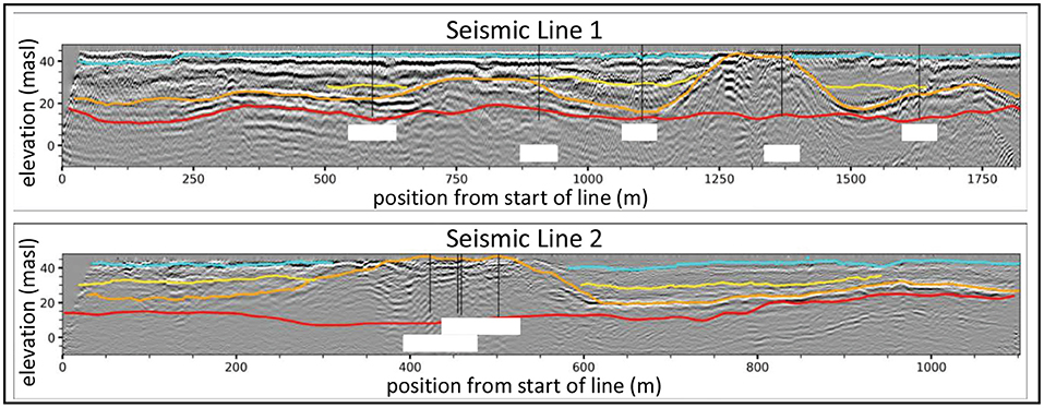
Figure 3. Two seismic reflection lines with 4 seismic horizons picked, from top to bottom: S3 (cyan), S2 (yellow), S1 (orange), and S0 (red).
The four seismic horizons are picked on all lines in two-way travel-time (TWT) and interpolated on a local 2D grid (10 m grid cells) at site by the discrete smooth interpolator (DSI; Mallet, 2002). Time-thickness maps between all seismic horizons are then computed. Associations between time-thickness maps and hydrostratigraphic units thickness are completed to allow combining with well markers for modeling units thickness and elevations. Referring to Figure 3, time-thickness between seismic horizon S3 and higher seismic horizon between S2 and S1 corresponds to the Marine Clay unit thickness. In a similar manner, time-thickness between the highest seismic horizon between S2 and S1 and seismic horizon S0 corresponds to the Esker Sand and Gravel unit thickness. Unfortunately, the seismic data does not allow to associate any time-thickness to the Till unit thickness.
Kriging with external drift is then used to translate the time-thickness maps to true thickness map using unit thickness computed using well markers from wells located within or at proximity to the seismic local grid. This KED step allowed to integrate the seismic data as another source of data with the same unit referential for interpolating the unit thickness throughout the model domain. The method to integrate the seismic thickness maps is similar to that used by Claprood et al. (2012) who combined seismic interpretation and well markers to build a conceptual model, by Tremblay et al. (2013) who characterized a leachate plume by integrating geophysical data with hydraulic and geochemical data, and later by Blouin and Gloaguen (2015) who delineated stratigraphic contacts during a hydrogeological study.
4.3. Modeling Esker Sand and Gravel Thickness
The data are kriged sequentially using the nested approach of priority representing the levels of uncertainty in the data for building the conceptual physical model. For each hydrostratigraphic unit, the system of priority establishes a sequential approach in building the conceptual model, using all data first, and allowing to deform the interpolation completed at the previous step to better fit the most reliable data. We discuss the methodology into more detail by presenting how the Esker Sand and Gravel unit thickness is interpolated within the model domain. This assumes the bedrock and Till unit elevations are already computed.
The most important hydrostratigraphic unit in the region is the Esker Sand and Gravel unit. It is a local aquifer of high, but spatially variable hydraulic conductivity outcropping at the surface at the site's project. This unit is also connected to the regional bedrock aquifer at few localized windows through the Till Unit within the model domain, and has a significant influence on local and regional groundwater flow system.
The interpolation of the Esker Sand and Gravel unit thickness is completed by two successive kriging steps. The first step is to interpolate the unit thickness with ordinary kriging using all available thickness data and geological constraints:
• Thickness computed from well markers (most reliable data),
• Thickness computed where the Esker Sand and Gravel is outcropping on the surface geology map (some uncertainty on this data),
• Thickness computed from high resolution seismic reflection data presented in the previous section (some uncertainty on this data),
• 0 m thickness where the Till unit is outcropping on the surface geology map.
All data, with low and high uncertainty, are considered in this first step of kriging to improve the modeling of large-scale structures. Seismic horizon are used to improve modeling the spatial structure of the Esker Sand and Gravel unit thickness between the well markers, despite their uncertainty related to the time resolution of seismic horizons picking.
The variogram is built using the unit thickness interpreted from well markers, seismic reflection data and surface geology map. It contains sufficient data on the mid and long range for interpolating the unit thickness over the esker extension. The variogram is build on 100 m lags, at 30°, 75°, 120°, and 165° azimuth directions. The experimental and modeled variograms for the Esker Sand and Gravel unit thickness are presented at Figure 4A.
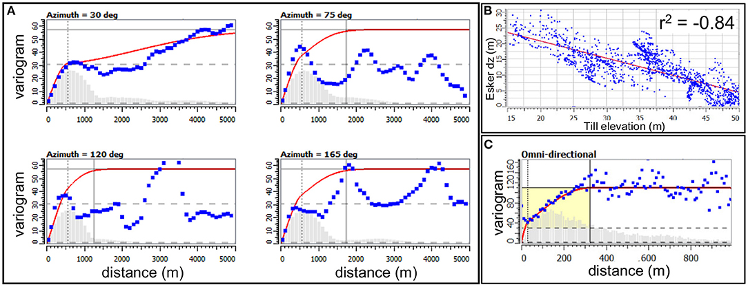
Figure 4. (A) Experimental and modeled variograms for Esker Sand and Gravel unit thickness computed on medium and long range data with all data available. (B) Crossplot between Esker Sand and Gravel unit thickness (Esker dz) and Till unit elevation (Till elevation). (C) Experimental and modeled variograms for Esker Sand and Gravel unit thickness computed on short range with well markers only.
The modeled variogram is a combination of 3 structures:
1. Nugget effect of contribution 0.7 m2,
2. Omnidirectional spherical model with a 550 m range, and a 30 m2 sill,
3. Gaussian model with a 5750 m maximum range at 30° azimuth, 1250 m minimum range, and a 27 m2 sill.
We detect a strong linear correlation between the Esker Sand and Gravel thickness and the elevation of the top of the Till Unit with a coefficient of correlation r2 = −0.84 (Figure 4B). The sand and gravel channels of the Esker unit being thicker in deeper pockets of Till unit.
This first interpolation of Esker Sand and Gravel thickness is completed by kriging with an external drift on a coarse grid of 100 m grid cells, using all unit thickness data available as primary data and the Till unit elevation map as external trend. To strengthen the relation between the Esker Sand and Gravel unit thickness and Till unit elevation, the azimuth of the principal direction of the variogram is allowed to vary according to the Till Unit elevation azimuth during the kriging process. This ensures the Esker Sand and Gravel unit fills in low elevation Till unit pockets, as expected during deposition of these high-energy glacial deposits, as the glacier most have follow the path of lowest elevation.
This first map of Esker Sand and Gravel unit thickness is then used as the regional trend which is allowed to be deformed locally to perfectly honor the Esker Sand and Gravel unit thickness interpreted at well markers, considered as the most reliable data. This second step is again completed by kriging with an external drift using a short range variogram built with well markers data only (Figure 4C).
The modeled variogram is a combination of 3 structures:
1. Nugget effect of contribution 1 m2,
2. Omnidirectional spherical model with a 30 m range, and a 28 m2 sill,
3. Omnidirectional spherical model with a 325 m range, and a 80 m2 sill.
The final map of Esker Sand and Gravel unit thickness is computed by KED on a 10 meter cells fine grid.
4.4. Modeling Hydrofacies With Seismic Reflection Data
While mostly undifferentiated in geological markers from most boreholes, geological description from newly acquired boreholes recognizes the presence of two main hydrofacies in the Esker Sand and Gravel unit; the main esker channels hydrofacies (F1_Esker) comprised of heterogeneous material with high and variable hydraulic conductivity, and the lateral silty and clayed sands hydrofacies (F2_SG) considered to be more continuous but having lower hydraulic conductivity than the main esker channels. As previously mentioned in section 4.2, these two hydrofacies could be differentiated from the seismic reflection data; the seismic horizon S1 is associated with the hydrofacies F1_Esker and the seismic horizon S2 is associated with the hydrofacies F2_SG.
To extrapolate the spatial distribution of these two hydrofacies outside the seismic grid, a multi-linear regression system was develop to find the most significant geometrical properties to predict the hydrofacies proportions. By training the model where the proportions of hydrofacies F1_Esker and F2_SG are known from seismic data, it is determined that a multi-linear regression equation combining the Marine clay unit thickness, the Esker Sand and Gravel unit thickness, the Till unit thickness, and the top of Esker Sand and Gravel elevation are most significant properties to predict the hydrofacies proportions in the conceptual physical model.
4.5. Integrating Well Logs
As presented in section 3.2, geophysical logs were recorded at nine wells at site during the pandemic summers of 2020 and 2021 to improve our knowledge on the vertical distribution of hydraulic parameters within the different hydrostratigraphic units.
Gamma ray and temperature logs are analyzed jointly to validate the structures seen on seismic data about the different units in the Quaternary sediments.
Gamma ray logs were also useful for dividing the bedrock unit in several sub-units with different proportions of clayey materials, which have an impact on the groundwater flow pattern. This will improve our conceptualization of the hydraulic parameters in the bedrock. Televiewer logs was also recorded to detect the quantity and direction of fractures within the bedrock.
The logs recorded in the bedrock suggest that a fractured bedrock with high hydraulic conductivity lies on top of clean bedrock with low hydraulic conductivity. The logs helped quantifying the level of fracturing into an equivalent matrix-based porosity for groundwater flow modeling, seen on the optical televiewer logs.
5. Results
The 3D conceptual model is built using all data available following the methodology presented in section 4. We present the results in three parts. The first part shows the impact of integrating high resolution seismic data by the nested sequential approach for reducing the uncertainty when modeling the lateral extents and thickness of the Esker Sand and Gravel unit. The second part shows the use of well logs to identify and different subunits within the bedrock. The final part shows the impact of integrating seismic reflection data and well logs on two cross-section of the 3D conceptual physical model.
5.1. Esker Sand and Gravel Unit
We present the results showing the integration of seismic reflection data for reducing the uncertainty in the representation of the Esker Sand and Gravel unit thickness map, following the method presented in sections 4.1 and 4.2.
Figure 5 presents two different versions of the Esker Sand and Gravel unit thickness map to analyse the impact of the high resolution seismic reflection on the interpolation. First version (Figure 5A) is the thickness map obtained without considering the seismic data, while the second version (Figure 5B) is obtained by considering the seismic data along with all other sources of data. Figure 5C presents the difference computed between the thickness map computed with and without the seismic data.
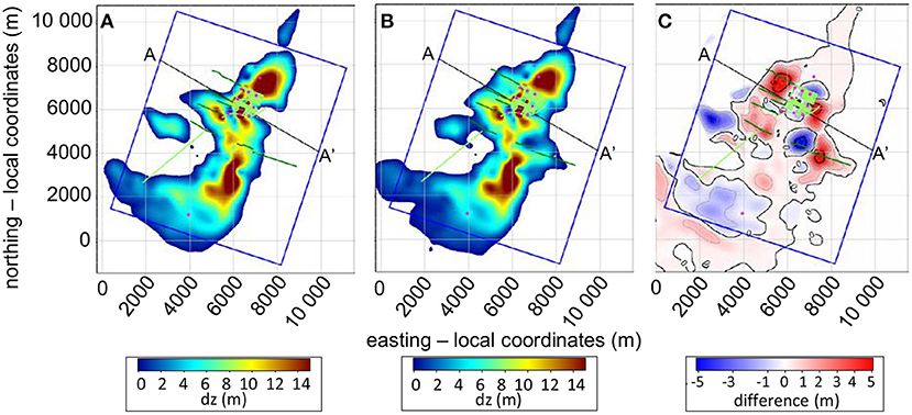
Figure 5. Esker Sand and Gravel unit thickness map not using (A) and using (B) the seismic reflection data. Panel (C) is the difference between (B) and (A). Black line is location of cross-section presented in Figure 8.
Figure 5 shows the impact of seismic reflection data to better delineate the lateral extents of the Esker Sand and Gravel unit. Seismic reflection data were useful to identify previously unknown esker branches which do not outcrop at surface, being located under some thickness of marine clay sediments. The total volume of sediments from the Esker Sand and Gravel unit was originally computed at 0.227 km3 in the model domain. After integration of seismic data, the volume of sediments from the Esker Sand and Gravel unit increases at 0.243 km3 in the model domain, an increase of 6%. This increase of high hydraulic conductivity material is likely to have a significant impact on the groundwater flow locally, especially in the pumping rate needed to catch the water in this area.
Because of the nature and spatial distribution of the data, a formal approach such as the multiple-fold cross-validation could not be used for this project. The cross-validation method is not applicable with data whose density range from very sparse regionally to very dense locally, especially when considering multiple sources of data with different resolution and spatial coverage. The reduction in uncertainty induced by the use of high resolution seismic data can be observed by the standard deviation maps (Figure 6).
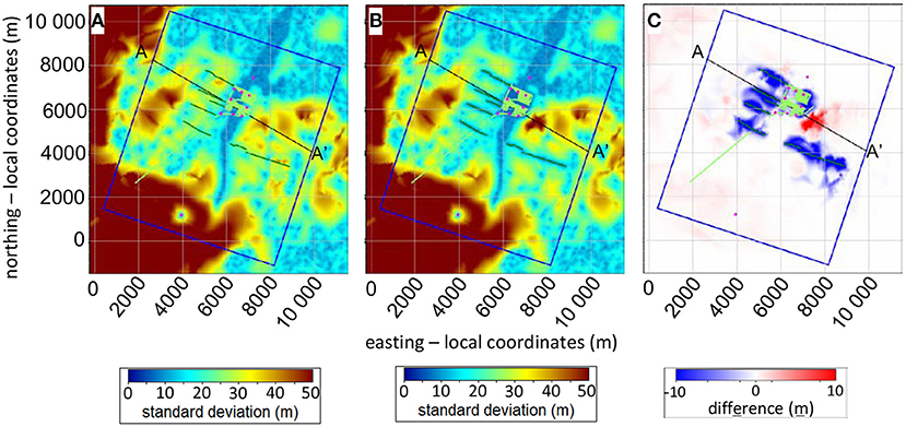
Figure 6. Standard deviation of the Esker Sand and Gravel unit thickness map not using (A) and using (B) the seismic reflection data. Panel (C) is the difference between (B) and (A). Black line is location of cross-section presented in Figure 8.
Low standard deviation indicates a greater confidence in the interpolation, and reduced uncertainty in modeling the thickness of the Esker Sand and Gravel unit. Even with as many wells locally at site, some uncertainty remains concerning the spatial variations in thickness of the esker, and its lateral continuity in the western and eastern edges, where the kriging variance increases (Figure 6A). As expected, a decrease of the in standard deviation is observed where seismic data have been recorded (Figure 6B). The standard deviation reduction reaches 10 m at several places within the model domain (Figure 6C).
5.2. Bedrock Sub-units
Well logs analysis indicates that the gamma-ray logs is well suited to identifying three distinct subunits within the bedrock, as well as a clear transitional marker between subunit 1 and subunit 2 (Figure 7).
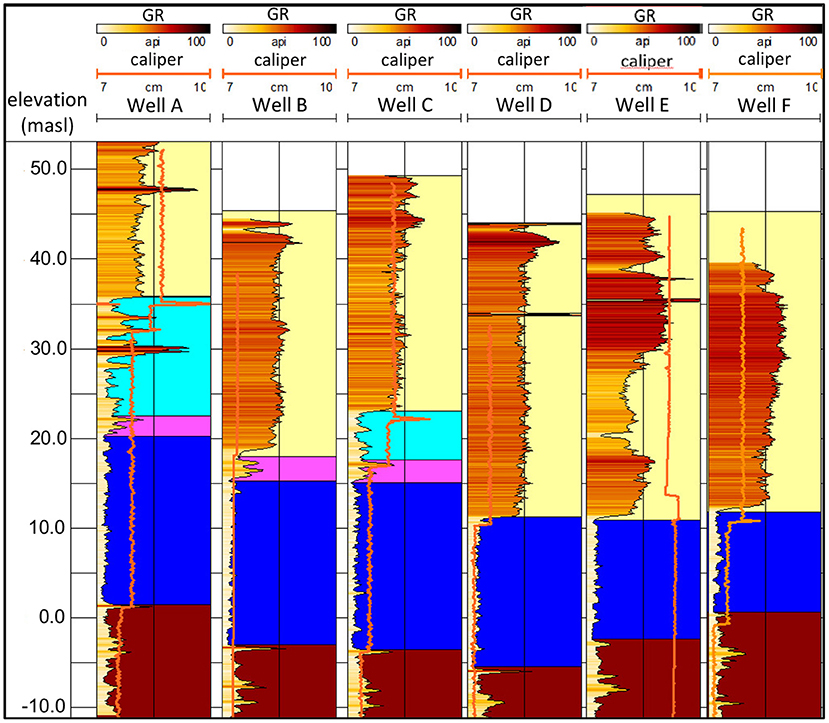
Figure 7. Identification of subunits in the bedrock from gamma ray well logs. Yellow zone is Quaternary sediments; turquoise zone is bedrock subunit 1; pink zone is transitional marker; blue zone is bedrock subunit 2; brown zone is bedrock subunit 3.
Wells A to F are all located at the site's project, within a few hundreds of meters of each other. The Quaternary sediments are highlighted in yellow zone. The turquoise zone above the transitional marker (magenta) is characterized by coarse grain material with important fractures density, and corresponds to subunit 1. It contains thin beds of shale material. The subunit 1 is eroded at most wells, being present only at Wells A and C. The subunit 2 is characterized by clean and small grain sediments with low shale content (low gamma-ray) and sub-horizontal fractures. The subunit 2 is present on all wells logs with a minimum thickness 10 m. It is expected to be present regionally and is represented in the conceptual physical model as a 10 meter thick layer below the Till unit and above the clean bedrock. It is the subunit where the groundwater flow is expected to be the greatest. The subunit 3 shows an increase on gamma-ray values, indication of higher shale or organic contents. This suggests a zonation within the subunit, lowering the groundwater flow. Further assessment with hydraulic testings in those bedrock units would allow to validate this interpretation.
5.3. 3D View
Figure 8 presents two different cross-section versions of the 3D conceptual physical model built by integrating all hydrostratigraphic units and bedrock sub-units.
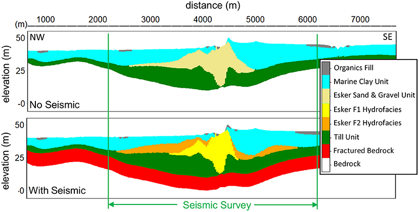
Figure 8. Northwest to southeast cross-sections of the 3D conceptual model without and considering the seismic data and well logs.
The cross-section on top shows the results without considering the seismic data, while the cross-section at the bottom shows the impact of acquiring high resolution seismic reflection data and well logs to better delimit the lateral extensions of the Esker Sand and Gravel unit, and represent the fractured bedrock subunit. The non-geophysically probed area was found to be drastically different when taking seismic data into account. Outside the new data, the two models are similar.
The representation of the two hydrofacies, F1_Esker and F2_SG, within the main hydrostatigraphic unit was possible with the acquisition of seismic reflection data. We compute that 24% of the Esker Sand and Gravel material is related to the F1_Esker hydrofacies, which spatial distribution will have an important role to play in the numerical modeling of groundwater flow at site, considering their distinct hydraulic conductivity distribution.
6. Discussion
The nested approach using successive steps of geostatistical interpolation method of kriging with external drift was critical to integrate data from multiple sources and to build the conceptual model of hydrostratigraphic units, considering the level of reliability of each set of data. While the kriging approach allows to integrate with minimum bias all data available while considering their uncertainty, the sequential approach permits to prioritize the fitting of the most reliable data available in the model, reducing the uncertainty when mapping the elevation and thickness of each hydrostratigraphic units.
Where few wells are present, high-resolution seismic reflection data was primordial to reduce the uncertainty linked to the spatial continuity of hydrostratigraphic units. The acquisition of seismic reflection data helped to better understand the structure of the paleo-glacial valleys and their lateral extensions while constructing the conceptual physical model of hydrostratigraphic units. Seismic reflection data were also used to identify and model the spatial distribution of two distinct hydrofacies in the main hydrostratigraphic unit. This will allow a better representation of the hydraulic conductivity, where its spatial distribution is expected to be significantly in both hydrofacies due to their different depositional environments. This will improve the reliability of the numerical model to predict the groundwater flow within the region of interest, leading to better calibrated parameters, and reduced uncertainty on the simulated groundwater flow for prescribed predicted scenarios.
The utility of well logs recorded at site is also advantageous in reducing the uncertainty. It helps to better constrain the hydraulic conductivity values by identifying three main subunits within the bedrock, each subunit having its own distribution of hydraulic conductivity. The division of the bedrock unit into subunits allows a more realistic parameterization of the hydraulic conductivity distribution within each subunit, which will reduce the uncertainty when building the numerical representation of the groundwater flow pattern.
7. Conclusions
The nested interpolation approach, and the use of high resolution seismic reflection data and well logs allow reducing the uncertainty and quantifying the improvement in representing the main hydrostratigraphic units when building the conceptual physical model at this undisclosed site.
The uncertainty has to considered at all steps of the project; building the hydrostratigraphic conceptual model, simulating the groundwater flow model, and calibrating the hydraulic parameters. This paper focussed on the first step of the project, building the conceptual physical model, but uncertainty will be quantitatively addressed when simulating the groundwater flow and calibrating the hydraulic parameters by data assimilation.
Data Availability Statement
The raw data supporting the conclusions of this article will be made available by the authors, without undue reservation.
Author Contributions
MCl contributed to modeling and writing of manuscript. EG contributed to conception and writing of manuscript. TB contributed to modeling, seismic interpretation, and statistical analysis of data. MB contributed to seismic acquisition, processing, and interpretation. CD contributed to well logs acquisition, processing, and interpretation. PF contributed to project conception and data organization. MO contributed to project conception. MCh contributed to data acquisition. RM contributed to project conception. DP contributed to project conception and multi-level slug tests acquisition and interpretation. JMB contributed to modeling and data analysis. All authors contributed to manuscript revision, read, and approved the submitted version.
Funding
Funding for the project was provided by a private contract from the Ministère de l'Environnement et de la Lutte contre les Changements Climatiques du Québec.
Conflict of Interest
The authors declare that the research was conducted in the absence of any commercial or financial relationships that could be construed as a potential conflict of interest.
Publisher's Note
All claims expressed in this article are solely those of the authors and do not necessarily represent those of their affiliated organizations, or those of the publisher, the editors and the reviewers. Any product that may be evaluated in this article, or claim that may be made by its manufacturer, is not guaranteed or endorsed by the publisher.
References
Ahokangas, E., Makinen, J., Artimo, A., Pasanen, A., and Vanhala, H. (2020). Interlobate esker aquifer characterization by high resolution seismic reflection method with landstreamer in SW Finland. J. Appl. Geophys. 177, 1–14. doi: 10.1016/j.jappgeo.2020.104014
Blouin, M., and Gloaguen, E. (2015). Comprehensive geophysical data integration and stratigraphic contacts delineation in a regional hydrogeological characterization study. J. Environ. Eng. Geophys. 20, 183–193. doi: 10.2113/JEEG20.2.183
Chen, J., Hubbard, S., and Rubin, Y. (2001). Estimating the hydraulic conductivity at the South Oyster site from geophysical tomography data using bayesian techniques based on the normal linear regression model. Water Resour. Res. 37, 1603–1613. doi: 10.1029/2000WR900392
Chilès, J.-P., and Delfiner, P. (1999). Geostatistics, Modeling Spatial Uncertainty. New York, NY: Wiley Series in Probability and Statistics. doi: 10.1002/9780470316993
Claprood, M., Gloaguen, E., Giroux, B., Konstantinovskaya, E., Malo, M., and Duchesne, M. J. (2012). Workflow using sparse vintage data for building a first geological and reservoir model for CO2 geological storage in deep saline aquifer. A case study in the St. Lawrence Platform, Canada. Greenhouse Gas Sci. Technol. 2, 260–278. doi: 10.1002/ghg.1292
Day-Lewis, F. D., Singha, K., and Binley, A. M. (2005). Applying petrophysical models to radar travel time and electrical resistivity tomograms: resolution-dependent limitations. J. Geophys. Res. 110:B08206. doi: 10.1029/2004JB003569
Dion, D.-J., Cocknurn, D., and Caron, P. (1986). Leve Geotechnique de la Region de Beauharnois-Candiac. Ministere de l'Energie et des Ressources du Quebec, Direction Generale de l'Exploration Geologique et Mineale.
Doherty, J., and Welter, D. (2010). A short exploration of structural noise. Water Resour. Res. 46, 1–14. doi: 10.1029/2009WR008377
Doyen, P. (2007). Seismic Reservoir Characterization, An Earth Modelling Perspective. Houten: European Association of Geoscientists and Engineers. doi: 10.3997/9789073781771
Dubrule, O. (2003). Geostatistics for Seismic Data Integration in Earth Models. Sponsored by the Society of Exploration Geophysicists and the European Association of Geoscientists and Engineers, Tulsa, OK. doi: 10.1190/1.9781560801962
Enemark, T., Peeters, L. J., Mallants, D., and Batelaan, O. (2019). Hydrogeological conceptual model building and testing: a review. J. Hydrol. 569, 310–329. doi: 10.1016/j.jhydrol.2018.12.007
Globensky, Y. (1986). Geologie de la Region de Saint-Chrysostome et de Lachine (SUD). Ministere de l'Energie et des Ressources, Quebec City, QC.
Gupta, H. V., Clark, M. P., Vrugt, J. A., Abramowitz, G., and Ye, M. (2012). Towards a comprehensive assessment of model structural adequacy. Water Resour. Res. 48:W08301. doi: 10.1029/2011WR011044
Inazaka, T. (2004). High resolution seismic reflection surveying at paved areas using an S-wave type Land Streamer. Explorat. Geophys. 35, 1–6. doi: 10.1071/EG04001
Lamontagne, C., and Nastev, M. (2010). Survol hydrogeologique de l'aquifere transfrontalier du bassin versant de la Riviere Chateauguay, Canada - Etats Unis. Can. Water Resour. 35, 359–376. doi: 10.4296/cwrj3504359
LaSalle, P. (1981). Geologie des Sediments meubles de la Region de Saint-Jean-Lachine. Ministere de l'Energie et des Ressources du Quebec, Direction Generale de l'exploration Geologique et Minerale.
Lavigne, M.-A. (2006). Modelisation Numerique de l'Ecoulement Regional de l'eau Souterraine Dans le Bassin Versant de la Riviere Chateauguay. INRS-ETE, Quebec City, QC.
Lavigne, M.-A., Nastev, M., and Lefebvre, R. (2010). Numerical simulation of groundwater flow in the Chateauguay River aquifers. Can. Water Resour. 35, 469–486. doi: 10.4296/cwrj3504469
Paradis, D., and Lefebvre, R. (2013). Single-well interference slug tests to assess the vertical hydraulic conductivity of unconsolidated aquifers. J. Hydrol. 478, 102–118. doi: 10.1016/j.jhydrol.2012.11.047
Paradis, D., Lefebvre, R., Morin, R. H., and Gloaguen, E. (2010). Permeability profiles in granular aquifers using flowmeters in direct-push wells. Groundwater 49, 534–547. doi: 10.1111/j.1745-6584.2010.00761.x
Pontlevoy, O. (2004). Modelisation Hydrogeologique pour Supporter la Gestion du Systeme Aquifere de la Region de Ville-Mercier. INRS-ETE, Quebec City, QC.
Pugin, A. J.-M., Oldenborger, G. A., Cummings, D. I., Russell, H. A., and Sharpe, D. R. (2014). Architecture of buried valleys in glaciated Canadian Prairie regions based on high resolution geophysical data. Q. Sci. Rev. 86, 13–23. doi: 10.1016/j.quascirev.2013.12.007
Pugin, A. J.-M., Pullan, S. E., and Duchesne, M. (2013). Regional hydrostratigraphy and insights into fluid flow through a clay aquitard from shallow seismic reflection data. Leading Edge 32, 742–748. doi: 10.1190/tle32070742.1
Pugin, A. J.-M., Pullan, S. E., Hunter, J. A., and Oldenborger, G. A. (2009). Hydrogeological prospecting using P- and S-wave landstreamer seismic reflection methods. Near Surface Geophys. 7, 315–328. doi: 10.3997/1873-0604.2009033
Rubin, Y., and Hubbard, S. S. (2005). Hydrogeophysics, Vol. 50. Dordrecht: Springer. doi: 10.1007/1-4020-3102-5
Sharpe, D. R., Pugin, A. J.-M., Pullan, S. E., and Gorrell, G. (2003). Application of seismic stratigraphy and sedimentology to regional hydrogeological investigations: an example from Oak Ridges Moraine, southern Ontario, Canada. Can. Geotech. J. 40, 711–730. doi: 10.1139/t03-020
Stockwell, J. W. (1999). The CWP/SU: Seismic Un*x package. Comput. Geosci. 25, 415–419. doi: 10.1016/S0098-3004(98)00145-9
Tremblay, L., Lefebvre, R., Paradis, D., and Gloaguen, E. (2013). Conceptual model of leachate migration in a granular aquifer derived from the integration of multi-source characterization data (St-Lambert, Canada). Hydrogeol. J. 22, 587–608. doi: 10.1007/s10040-013-1065-1
Tremblay, T. (2008). Hydrostratigraphie et Geologie du Quaternaire dans le Bassin-Versant de la Riviere Chateauguay, Quebec. Universite du Quebec e Montreal, Departement des Sciences de la Terre.
Tremblay, T., Hunter, J., Lamontagne, C., and Nastev, M. (2010). High resolution seismic survey in a contaminated esker area, Chateauguay river watershed, Quebec. Can. Water Resour. J. 35, 417–432. doi: 10.4296/cwrj3504417
Tremblay, T., and Lamothe, M. (2005). Geologie des Formations Superficielles du Bassin-Versant de la Riviere Chateauguay. Universite du Quebec e Montreal.
Van der Veen, M., Spitzer, R., Green, A., and Wilde, P. (2001). Design and application of a towed landstreamer for cost-effective 2D and pseudo-3D shallow seismic data acquisition. Geophysics 66, 482–500. doi: 10.1190/1.1444939
Keywords: seismic reflection, well logs, conceptual model, geological structure, hydraulic properties, uncertainty, groundwater flow
Citation: Claprood M, Gloaguen E, Béraud T, Blouin M, Dupuis C, Ferron P, Ouellet M, Chaussé M, Martel R, Paradis D and Ballard J-M (2022) A Case Study Using Seismic Reflection and Well Logs to Reduce and Quantify Uncertainty During a Hydrogeological Assessment. Front. Water 3:779149. doi: 10.3389/frwa.2021.779149
Received: 18 September 2021; Accepted: 09 December 2021;
Published: 09 February 2022.
Edited by:
Yoram Rubin, University of California, Berkeley, United StatesReviewed by:
Luk J. M. Peeters, CSIRO Land and Water, AustraliaJinsong Chen, Lawrence Berkeley National Laboratory, United States
Copyright © 2022 Claprood, Gloaguen, Béraud, Blouin, Dupuis, Ferron, Ouellet, Chaussé, Martel, Paradis and Ballard. This is an open-access article distributed under the terms of the Creative Commons Attribution License (CC BY). The use, distribution or reproduction in other forums is permitted, provided the original author(s) and the copyright owner(s) are credited and that the original publication in this journal is cited, in accordance with accepted academic practice. No use, distribution or reproduction is permitted which does not comply with these terms.
*Correspondence: Maxime Claprood, bWF4aW1lLmNsYXByb29kQGlucnMuY2E=