Validation and Projections of Climate Characteristics in the Saginaw Bay Watershed, MI, for Hydrologic Modeling Applications

Kluver, Daria B.; Robertson, Wendy

doi:10.3389/frwa.2021.779811

ORIGINAL RESEARCH article

Front. Water, 24 December 2021

Sec. Water and Climate

Volume 3 - 2021 | https://doi.org/10.3389/frwa.2021.779811

This article is part of the Research Topic Hydroclimatology of the Great Lakes Region of North America View all 16 articles

Validation and Projections of Climate Characteristics in the Saginaw Bay Watershed, MI, for Hydrologic Modeling Applications

$\nDaria B. Kluver,$ Daria B. Kluver^1,2^*

Wendy Robertson^1,2

¹Department of Earth and Atmospheric Sciences, Central Michigan University, Mount Pleasant, MI, United States
²Institute for Great Lakes Research, Central Michigan University, Mount Pleasant, MI, United States

Fundamental differences in the nature of climate and hydrologic models make coupling of future climate projections to models of watershed hydrology challenging. This study uses the NCAR Weather Research and Forecast model (WRF) to dynamically downscale climate simulations over the Saginaw Bay Watershed, MI and prepare the results for input into semi-distributed hydrologic models. One realization of the bias-corrected NCAR CESM1 model's RCP 8.5 climate scenario is dynamically downscaled at a spatial resolution of 3 km by 3 km for the end of the twenty-first century and validated based on a downscaled run for the end of the twentieth century in comparison to ASOS and NWS COOP stations. Bias-correction is conducted using Quantile Mapping to correct daily maximum and minimum temperature, precipitation, and relative humidity for use in future hydrologic model experiments. In the Saginaw Bay Watershed the end of the twenty-first century is projected to see maximum and minimum average daily temperatures warming by 5.7 and 6.3°C respectively. Precipitation characteristics over the watershed show an increase in mean annual precipitation (average of +14.3 mm over the watershed), mainly due to increases in precipitation intensity (average of +0.3 mm per precipitation day) despite a decrease in frequency of −10.7 days per year. The projected changes have substantial implications for watershed processes including flood prediction, erosion, mobilization of non-point source and legacy contaminants, and evapotranspirative demand, among others. We present these results in the context of usefulness of the downscaled and bias corrected data for semi-distributed hydrologic modeling.

Introduction

Climate change has the potential to substantially alter the abundance, availability, distribution, fluxes, and quality of water in the Great Lakes region (Hayhoe et al., 2010; D'Orgeville et al., 2014; Byun and Hamlet, 2018; Wang et al., 2018; Byun et al., 2019; Mahdiyan et al., 2021). Increases in extreme weather events, changes in the timing, type, and spatial distribution of precipitation, and alterations to evapotranspirative fluxes all have implications for streamflow and water quality. Effects of climate change on hydrologic extremes such as drought and flooding have the potential to compound existing stressors in Great Lakes watersheds already impacted by decades of land use change, legacy and non-point source pollution, and loss of wetland habitat. Predictions from global scale climate modeling establish that rising temperatures will result in changes to the atmospheric characteristics in the Great Lakes region that will have direct effects on watershed health, such as increases in extreme precipitation and droughts (which impacts erosion, nutrient cycling, and flux of pollutants), increased temperatures (impacts to phenology, ecology, and agriculture), and changes to soil moisture (impacting nutrient cycling, hydrologic fluxes, phenology, and water quality; Angel et al., 2018). However, there remains significant uncertainty in how the projected climate changes modeled at the global scale translate to hydrologic impacts at the regional and watershed scales. One reason that uncertainty persists is the fundamentally different nature of global climate models (GCMs) and hydrologic models. While GCMs are applied at global scales for long periods of time, many of the processes that scientists and policy makers seek to model for watersheds, such as daily streamflows for ecological minimums and flood event timing and magnitude, are much smaller in extent and discrete in time. The contrast between spatial and temporal resolutions and modeling approaches poses challenges for model coupling. However, the gap between these two modeling paradigms is worth bridging, particularly for understanding the complex nature of changes in Great Lakes watersheds in response to future climate change. One notable effort toward reconciling the challenge of coupling atmospheric and terrestrial hydrologic models is WRF-Hydro, which provides high resolution (both spatially and temporally) streamflow predictions on short (sub-hourly) to seasonal time scales (Lin et al., 2018; Somos-Valenzuela and Palmer, 2018; Yin et al., 2020). A significant drawback to the WRF-Hydro modeling framework is that it is extremely computationally intensive to get streamflow in a fully or semi-distributed representation of a catchment which becomes prohibitive over the climate-scale simulations required to realize future hydrologic distributions.

Because GCMs use physical principles of the atmosphere to drive long-term simulations of climate variability and change (rather than observations, such as in Numerical Weather Prediction), they are computationally intensive, and must therefore be of a coarse spatial resolution, generally greater than 1° latitude by 1° longitude. Their purpose is to capture the physical processes that occur over the entire globe at timescales greater than weather forecasts and to indicate broad regional changes to climate parameters. Inputs and output are in the form of gridded fields at specific points in time. By contrast, hydrologic models are frequently applied to explore watershed and stream response to changes at the basin scale, which depending on the size of the catchment can range from as small as the contributing area to a local stream to as large as continental scales. Hydrologic models can be conceptual (based on physical concepts), empirical, or physically based and can range both in complexity of modeled processes and spatial distribution. To explore how streamflow responds to variations in watershed characteristics and perturbations such as land use and climate change, physically based distributed or semi-distributed hydrologic models (SDHMs) are necessary (Jajarmizdeh et al., 2012; Khakbaz et al., 2012). A benefit SDHMs can provide is prediction of streamflow in ungauged catchments, a capability that is critical where monitoring networks are sparse. SDHMs require input of spatially explicit datasets including watershed properties such as soil, topography, and land use, and climatological inputs such as precipitation, temperature, solar radiation, wind speed, and relative humidity. The type and detail of inputs varies between models; fully distributed models may use gridded data for all inputs, whereas semi-distributed models can incorporate both gridded and point data (which is then interpolated to provide the necessary input). For most SDHM applications, climatological inputs come from existing observation stations (e.g., NWS COOP network in the U.S.) or gridded products (e.g., CFSR; National Center for Atmospheric Research Staff, 2017). However, these inputs are not available for future conditions; this is where GCM or Regional Climate Model (RCM) output links to SDHMs (e.g., Das and Umamahesh, 2018; Singh and Saravanan, 2020; Martínez-Salvador et al., 2021); in these cases, resolving the difference in spatial resolution remains a challenge. To model hydrologic response to future climate conditions, climatological inputs based on those future conditions are needed. It is imperative that the climatological inputs are as representative of likely future atmospheric conditions (given a particular emissions scenario) as possible, as calibration of SDHMs relies on altering empirical fit parameters linked to physical characteristics and properties of the watershed rather than correction of climatological inputs (Arnold et al., 2012; Zhai et al., 2018; Gou et al., 2020). To take the low-resolution gridded outputs produced by GCMs and prepare them in such a way as to capture accurate sub-grid scale variability for hydrologic modeling is no simple task. It involves some form of downscaling to a resolution that is useful for quantifying watershed-scale variability, but also validation and bias correction from in-situ “ground truth” stations at such a resolution, which requires the transition from gridded spatial data to spatially explicit (point) data.

In order to address the challenge of coupling GCMs to hydrologic models, researchers have turned to two main approaches: statistical (empirical) and dynamic downscaling (Hewitson and Crane, 1996). Statistical downscaling involves development of empirical relationships between outputs from a course resolution GCM (a predictor) and a historic data set (a predictand). The type of statistical model used to define this relationship can vary, but is limited in that it does not represent the atmospheric processes that link the two scales together (large scale to local scale; Maraun and Widmann, 2018). Dynamical downscaling on the other hand is process-driven and is conducted via nested climate/weather models of progressively smaller domain and finer resolution [these can then be called Regional Climate Models (RCMs)]. While statistical downscaling is computationally much more efficient, dynamical downscaling has the ability to adapt to complex changes in future climate—assuming the relevant processes are represented in the model.

Dynamically downscaled climate model outputs have been used as inputs into several distributed and semi-distributed hydrologic models to address changes in physical characteristics and properties that impact streamflow (e.g., rainfall-runoff ratio, snowmelt timing, and evapotranspirative demand) as well as extreme events (e.g., drought, flood risk, and extreme precipitation; Salathe et al., 2014; Mendoza et al., 2015; Vu et al., 2015 and others). Recent studies that have used downscaled climate model output in such a manner have taken a number of approaches. Most commonly the variables retained from the model output are limited to monthly mean temperature and precipitation [with the exception of Erler et al. (2019), which uitilized mean monthly precipitation, snow depth and PET in the HydroGeoSphere model]. Raghavan et al. (2014), Vu et al. (2015), and Tiwari et al. (2018) passed climate output fields to the SWAT hydrologic model un-corrected, and calibrated SWAT to make up for any discrepancies between modeled and observed stream gauge data. Shrestha et al. (2017) took another approach and found that applying simple corrections to only modeled temperature and precipitation improved hydrologic model performance (they also used SWAT).

The main limitations to the previous body of work revolve around incorporating the processes that are evolving in the atmosphere in future states of the climate with the impacts of those processes on hydrologic systems. Without a GCM that is based on coupled atmospheric, land, and ocean components, future climate estimates are likely to miss global- and hemispheric-scale drivers of climate, such as the El Niño Southern Oscillation, Arctic Oscillation, sea ice fluctuations, and others. However, the GCMs that are capable of simulating these global-scale processes are substantially mismatched in spatial resolution with the types of systems usually modeled in SDHMs. Such a mismatch will result in instances where GCMs and coarse-resolution RCMs are not capturing the sub-watershed spatial variability even if the atmospheric processes are accurately represented at the larger grid scale. This can leave out atmospheric drivers of hydrologic processes of interest, such as erosion, non-point source pollution, land use stressors, and point source pollutant mobilization.

This study presents a unique approach to addressing some of the challenges posed by the existing methodologies for preparation of future climate projections for coupling with hydrologic SDHMs. One realization of a GCM's projections of future climate are dynamically downscaled with a high-fidelity weather model, to retain the physical processes occurring within the atmosphere at subsequently smaller spatial and temporal resolutions. This is done at a very high resolution, with the inner-most domain having grid cells of 3 km by 3 km. After downscaling, bias correction is applied to atmospheric variables at locations within the watershed to leverage the in-situ observations available to provide improved atmospheric forcing for the hydrologic model, thereby reserving hydrologic model calibration for the streamflow parameters. Lastly, the steps for data preparation are applied to several variables (maximum temperature, minimum temperature, daily precipitation, and relative humidity) due to their potential to alter components on hydrologic systems such as flooding, ET demand, soil moisture storage, runoff, infiltration, nutrient cycling, and water levels.

In this paper, we focus on an example from the Saginaw Bay watershed in the lower peninsula of Michigan. We use the NCAR Weather Research and Forecast model (WRF) to dynamically downscale CMIP5 output to a nested domain of 3 km grids centered over the Great Lakes region, running this weather model as an RCM. We ran two 15-year periods; one at the end of the twentieth century and one at the end of the twenty-first century using RCP 8.5 to quantify climate change impacts on the region and explore the variability of such changes over a high spatial resolution within the watershed, which would not be captured in statistically downscaled climate output. Then, we applied quantile mapping to the precipitation, daily maximum and minimum temperatures, and relative humidity to bias correct the variables prior to using them as input for hydrologic modeling.

Data and Methods

Study Area

The Saginaw Bay Watershed (SBW) is located in the eastern part of Michigan's lower Peninsula (Figure 1). It is the largest drainage basin in the state of Michigan, encompassing approximately 14,000 km², 22 counties, and a wide range of land uses from highly urbanized to agricultural and forested. Its outlet, Saginaw Bay, provides habitat for multiple federal and state recognized threatened and endangered species including resident and migratory birds, reptiles, insects, aquatic invertebrates, and plant species (U.S. Fish Wildlife Service., 2018; Michigan Natural Feathers Inventory) and is also a U.S. EPA designated Area of Concern with ongoing Beneficial Use Impairments (BUIs) related to nonpoint source pollution and legacy contamination in the sediments (Selzer et al., 2014). Eutrophication, nuisance algal blooms, beach closures, and ecosystem degradation are current challenges that also may be exacerbated by climate change impacts within the watershed. Many of the tributaries in the SBW are prone to rapid hydrologic response (Michigan Department of Natural Resources Surface Water Quality Division, 1988; Selzer et al., 2014) resulting from land use changes and low permeability soils; the “flashy” response may be compounded by climatic shifts, and, also have the potential to contribute to sediment and non-point source pollutant loading, negatively impacting water quality conditions and ecosystem services in Saginaw Bay.

FIGURE 1

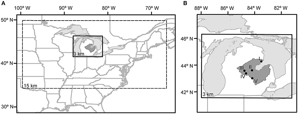
Figure 1. Study area. (A) WRF downscaled domains, outer domain (dashed line) and inner domain (solid line). (B) Location of in-situ weather stations in relation to the Saginaw Bay Watershed: I. East Tawas/Oscoda, MI; II. Midland, MI; III. Mount Pleasant, MI; IV. Alma/Gratiot, MI; and V. Owosso, MI.

The climate of this region is largely influenced by its position in the mid-latitude Westerlies, with sizable influence from the surrounding Great Lakes. The large bodies of water that surround the Michigan Lower Peninsula on 3 sides act to moderate the temperatures in this region, but also act as a moisture source for precipitation. Despite the maritime effect from the Great Lakes, in the last century Michigan has still experienced increasing annual temperatures of around 0.8°C and future warming is projected to be as much as 5.4°C (for RCP 8.5) by 2099 (Wuebbles et al., 2019). Precipitation is achieved in the SBW through transient synoptic weather patterns (such as fronts, or mid-latitude cyclones) or the moistening of cold air masses as they pass over the Great Lakes (Andresen, 2012). Over the twentieth century annual precipitation in the SBW region has increased by as much as 15% (Wuebbles et al., 2019), mostly due to the increases in extreme precipitation event sizes (Easterling et al., 2017). Future projections continue this trend of more annual precipitation, primarily due to extreme events (Wuebbles et al., 2019). When examining the CMIP5 suite of GCMs' projections for the Great Lakes region, Notaro et al. (2015) found that the maximum precipitation increases by the end of the twenty-first century (RCP 8.5) occurred in March–April–May and were +0.61 mm day⁻¹ compared to late twentieth century values. Increases in temperature were also documented, with a maximum warming of +7.0°C occurring in December–January–February.

Downscaling

The NCAR Weather Research and Forecast (WRF) model (version 3.7) with the Advanced Research WRF (ARW) core dynamical solver (Skamarock et al., 2008) is used to model the atmospheric parameters over the SBW. The WRF model is configured with the following physics schemes: the unified Noah Land Surface Model for surface physics (Tewari et al., 2004); the NCEP GFS boundary layer physics (Hong and Pan, 1996); the Kain-Fritsch convection scheme (applied to both domains; Kain, 2004); the Dudhia shortwave radiation scheme (Dudhia, 1989); the Rapid Radiation Transfer Model for longwave radiation (Mlawer et al., 1997); and the WRF Single-Moment 5-Class scheme for microphysics (Hong et al., 2004). Nudging is not applied in an effort to preserve precipitation variability within the inner domain (Alexandru et al., 2009), although it has been shown by multiple studies to improve WRF downscaling simulations of 1–3 year periods (Spero et al., 2018). The Climate simulations from the NCAR CESM Global Bias-Corrected CMIP5 Output to Support WRF/MPAS project (Monaghan et al., 2014) are used as initial boundary conditions for the WRF model. These data are bias-corrected using the ECMWF ERA-Interim from 1981 to 2005 (Bruyère et al., 2014, 2015) and are available for the IPCC AR5 RCP 4.5, 6.0, and 8.5 scenarios from 2006 to 2100. A simulation from 1950 to 2005 is also used to calibrate the GCM model and is available as a twentieth century run.¹ The bias-corrected CESM data set is useful, because systematic biases in the Great Lakes region can vary by season (too wet in winter and spring and too dry in fall) and be large (as much as −13% fall precipitation bias from CESM1; Briley et al., 2020). In all WRF model runs the 1° CESM1 6-hourly output files are used as the boundary conditions for an outer domain of 15 km horizontal grids and then are dynamically downscaled to a two-way nested inner domain of 3 km horizontal grids (shown in Figure 1). The WRF model was developed as a high-resolution weather forecasting tool (shorter time scales but higher spatial resolution) and has since started to be used as an RCM, sometimes simulating time periods as long as those used in this study. The advantage of using WRF in this application is its ability to simulate at a spatial resolution that is sufficient to represent atmospheric processes, such as precipitation, that are usually considered “sub-grid scale” for long-term global climate models (Wang and Kotamarthi, 2015). The trade-off to using this model is the cost of computation and data storage to produce such fine spatial-scale but long runs.

Due to the computationally demanding nature of numerical weather models, only one realization of the WRF model is run for two different 15-year periods. The first is a twentieth Century simulation from 1991 to 2005 for use in model validation, which we will refer to as the ‘historical' run. The second 15-year WRF run is using the RCP 8.5 future scenario, simulated from 2085 to 2099, which assumes an increase in radiative forcing of +8.5 W/m2 over pre-industrial values (Van Vuuren et al., 2011; Stocker et al., 2013; Bruyère et al., 2014). We will refer to this run as the “future” run. Notaro et al. (2015) assessed the uncertainty in CMIP5 models over the Great Lakes region for this time period. They found that the deviation among the models in the end-of-twenty-first century RCP 8.5 scenario runs resulted in an average temperature and precipitation uncertainty of 1.29°C and 0.20 mm day⁻¹. For both WRF model runs the daily variables retained for future input into SDHMs are: maximum temperature (°C); minimum temperature (°C); total liquid precipitation (mm); average relative humidity (%); and average daily wind speed (m/s) computed for each grid cell in the SBW domain. Wind speeds are reduced to 2-m height and adjusted to account for varying ground cover types using the Prandtl-von Karman Universal Velocity-Distribution for Turbulent Flows (Dingman, 2008). The friction velocity for the vegetation types are based on previous field experiments (Izumi and Caughey, 1976; Churchill and Csanady, 1983; Santoso and Stull, 2001; Jiao-jun et al., 2004). For the basin-wide figures and statistics, WRF output grids are clipped to only those within the Saginaw Bay Watershed, with a 1,000 m buffer for the centroids falling within the boundary of the watershed (n = 2582).

Validation and bias correction of the downscaled atmospheric variables is essential at the points for which data will be passed to the SDHM, because the coarse resolution GCMs lack some sub-grid scale features. One relevant shortcoming of the CMIP5 models (and this CESM1 contribution to CMIP5 in particular) is the lack of lake surface temperatures included in the output files for use in regional downscaling (Spero et al., 2016). Without lake water temperatures from the input GCM, the WRF model defaults to extrapolating water temperature from the nearest point designated as water. In this situation, different portions of the Laurentian Great Lakes are interpolated from grid cells over the Atlantic Ocean (southern lake areas), or from James and Hudson Bays (northern lake areas; Mallard et al., 2015; Spero et al., 2016). Mallard et al. (2015) found discontinuities in lake surface temperature of as much as 17 K in Lakes Michigan and Huron, and 3 K in Lake Superior during one simulated test date. Spero et al. (2016) examined the same CESM1 model used in the current study and found lake temperatures that were colder in the summer and warmer in the winter, compared to a WRF downscaling that included a lake model. The largest impacts were in the winter, where thermally induced low pressure and warmer air temperatures downwind of the lakes impacted the frequency of freeze days and number of days with precipitation (Spero et al., 2016). Since the default WRF treatment of “water” grids is used in the current study, careful validation and bias correction are of the utmost importance.

Bias Correction

WRF model validation is conducted by comparing the WRF downscaled model output against historical climate station data from the in-situ stations from the National Weather Service Cooperative Observer Program (NCEI., 2017), and wind data from the NOAA's Automated Surface Observation Stations (ASOS) locations (NCEI, 2019). The locations of the stations that have both COOP and ASOS data and lie inside the Saginaw Bay Watershed (SBW) are given in Figure 1. Errors are computed only at model grid cells that are co-located with historic in-situ stations, in order to avoid any potential bias that may be introduced by interpolation during error estimation or correction. However, it should be noted that since spatial autocorrelation decreases with distance, the representativeness of co-located in-situ stations and model grid cells can vary if station locations are offset by only a few tenths of a degree latitude or longitude. These historic in-situ locations are subsequently the only grid cells bias-corrected for ingest into a SDHM. The Kolmogorov-Smirnov test is conducted on each set of distribution comparisons to identify whether they could statistically be from the same distribution (Schuenemeyer and Drew, 2011).

After errors are identified in the historic run, by comparing the downscaled WRF output to the observational stations, bias correction is performed. We apply bias correction on temperature, precipitation, and humidity variables. Relative humidity is not often included or bias corrected for in GCM-hydrologic model coupling, however, Masaki et al. (2015) found that bias correction of humidity (even simplistic methods) reduce uncertainty in hydrologic models. Of the recent studies that have conducted bias correction on WRF data for use in hydrologic models, the majority used a gridded dataset or gridded historical observations as their ground truth. The interpolation of the historical station data to produce such a dataset can introduce additional biases, particularly for precipitation, which has increased interpolation error with increased station distances (Bussieres and Hogg, 1989). For this paper, the WRF grid cells that correspond to historical weather station locations are the ones at which bias correction is applied as these would be a standard input for climate variables into a SDHM.

Because the entire range of the statistical distributions of the variables that are input into the hydrologic model has implications for hydrologic processes within the watershed and therefore streamflow, quantile mapping is used for bias correction. Compared to the more commonly used change factor (add or subtract model anomalies from observations), the quantile mapping method allows for the amount of correction applied to the model data to vary along the distribution. The quantile mapping method of bias correction (Boé et al., 2007; Gudmundsson et al., 2012; Gudmundsson, 2014) estimates the empirical cumulative distribution function (ecdf) of both the modeled and observed variables. The model data is then corrected (or transformed) at the specific quantiles (we used every 10th percentile), and intermediate values must be interpolated (in this study, the non-linear monotonic tricubic spline interpolation is used; Gudmundsson et al., 2012; Mosier et al., 2014, 2018; Sippel et al., 2016; Alidoost et al., 2021). This produces a bias correction that is tailored to the correction needs at different levels in the distribution, rather than one correction applied unilaterally. This is particularly useful for distributions that require different corrections for the tails of the distributions compared to the means of the distributions, as the tails represent flood and drought conditions that can have important devastating impacts on hydrologic systems.

Results

WRF Simulations of the SBW: 1991–2005 and 2085–2099

Annual average watershed values produced from the 1991 to 2005 historical WRF run are shown in Figure 2A through Figure 7A and future WRF model run in Figure 2B through Figure 7B. In order to examine the spatial changes projected to occur, annual average values from the entire modeled watershed are compared for the twentieth century run to the end of the twenty-first century RCP 8.5 run and the change is displayed in Figure 2C through Figure 7C. Empirical distributions are generated from the grid cell values over the watershed to show the distribution of the data throughout the study area and how it changes between the two time periods (Figure 2D through Figure 7D).

FIGURE 2

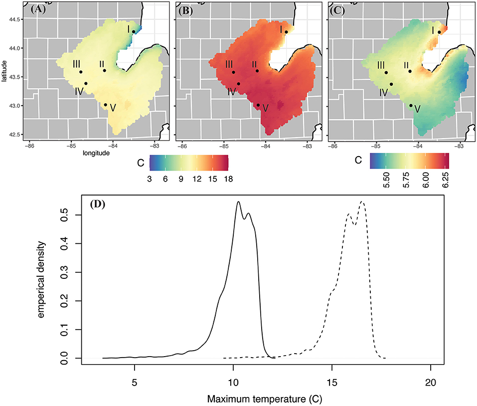
Figure 2. Uncorrected WRF output of mean maximum daily temperature (°C) from (A) the 1991–2005 historical climate run; (B) the 2085–2099 future RCP 8.5 scenario; (C) the difference between the (A) and (B) future–past and (D) the empirical distribution from all of the grid cells in the watershed for mean maximum daily temperature for (A) (solid line) and (B) (dashed line).

For the historic WRF run the variables plotted show a spatially reasonable pattern, with cooler average maximum and minimum temperatures along the shores of the Saginaw Bay (3.8 and −5.3°C, respectively) and increased temperatures westward (11.7 and 1.5°C, respectively; Figures 2A, 3A). Not only are the areas around the bay cooler, but they experience higher relative humidity (~86% compared to 71.5% inland; Figure 4A). Precipitation characteristics around Saginaw Bay are also distinctly different than the inland part of the SBW. WRF grid cells near the bay experience precipitation more frequently (~210 days/year compared to ~176 days/year; Figure 6A), but at a lower intensity (3.69 mm/rain day compared to 5.14 mm/rain day; Figure 7A), resulting in lower total amounts of precipitation than inland (~739 mm compared to 995.4 mm; Figure 5A).

FIGURE 3

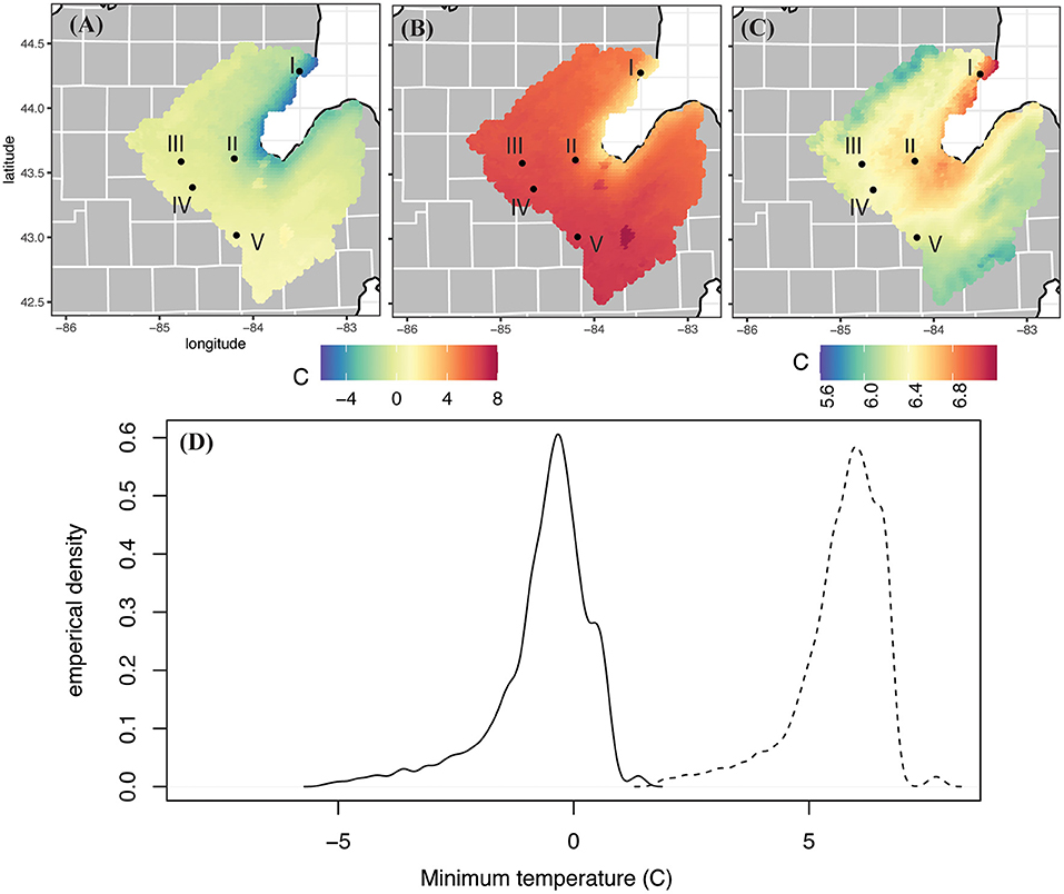
Figure 3. Same as Figure 2, but for minimum daily temperature.

FIGURE 4

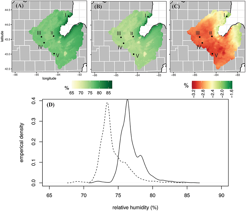
Figure 4. Same as Figure 2, but for mean daily relative humidity.

FIGURE 5

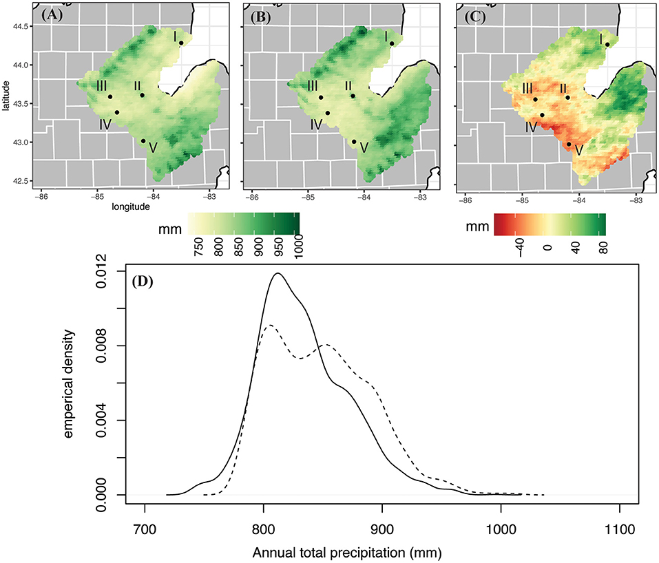
Figure 5. Same as Figure 2, but for annual total precipitation amount.

In Figure 2B, future mean maximum temperatures across the SBW range from 17.3°C in the western portion of the watershed, to as low as 10.0°C along the Saginaw Bay. The mean value across the entire watershed is 15.8°C, with a standard deviation of 0.89 °C. Comparing this spatial distribution to the historic model run (Figure 2A), annual average maximum temperatures in the SBW shows a mean change of 5.7°C by the end of the twenty-first century for the RCP 8.5 scenario. The spatial difference map (Figure 2C) shows the warming is largest along the coast of the Saginaw Bay (highest warming in a single grid cell is 6.1°C) and lowest in “the Thumb” area of 5.4°C. The empirical distributions created from the grid cells in each watershed map show that the entire distribution of temperatures shifts to higher temperatures, putting the majority of grid cells at temperatures above even the warmest maximum temperatures in the historic time period (Figure 2D).

The change signal in minimum temperatures is similar to maximum temperatures (Figure 3). Future values of minimum temperature over the SBW range from a minimum value of 1.7°C to a maximum value of 7.8°C, with a watershed average 5.7°C. The average minimum temperature in the watershed is projected to increase by 6.3°C from the historic run. The map shows that these increases are the highest around the coast (7.1°C), and lowest in the southeast and northwest edged of the watershed (5.9°C). The empirical distribution shows that nearly all grid cells in this watershed experience minimum temperatures in the future time period above even the extreme minimum temperatures in the historic model run.

A slight reducing pattern is projected to occur in relative humidity across the SBW by the end of the century, as can be seen in Figure 4B. The maximum average relative humidity in the future WRF run is 83.9%, compared to 86.1% in the historic run, occurring along the Saginaw Bay. When compared to the historic run (Figures 4A,C), the drying signal appears the smallest (−1.9%) on the northern coast of the Saginaw Bay and is the largest (−3.1%) in the southwestern corner of the watershed, near Owosso, MI (station V). The empirical distribution shows a future shift of ~2.7% drier in the future (watershed mean RH goes from 77.1 to 74.4%).

The northeastern side of the SBW is projected to receive more total annual precipitation by the end of the twenty-first century than it experienced in the historic model run (Figure 5B). When comparing the future projection map to the historic model run, the watershed's average increase of 14.3 mm (848.0 mm vs. the historic run's 833.7 mm) does not convey the spatial variability within the SBW. Particularly, drying occurs in the south and southwestern parts of the watershed, while moistening is isolated to the northeastern part of the SBW (Figure 5C). The maximum change over the twenty-first century at a single grid cell is an increase of 87.4 mm, and the largest drying is −63.0 mm. Figure 5D shows a flattening of the empirical distribution curve in the future model projections, with fewer grids having a precipitation value near the average, and more years with annual precipitation amounts occurring in the right tail of the curve. The reason for this can be more clearly seen by examining precipitation frequency and intensity.

Annual precipitation frequency (number of days with measurable precipitation per year) decreases in a future RCP 8.5 scenario at all grid cells in the Saginaw Bay Watershed (Figure 6) with a range of 4.7 to 24.4 fewer days per year. The average over the entire watershed is a decrease in precipitation frequency of 10.7 days per year. The empirical distributions show a similar shape to the two distributions, but the future distribution is shifted left (toward a lower frequency of days with precipitation) and the right tail of the distribution becomes shorter (fewer extremely high frequency years; Figure 6D).

FIGURE 6

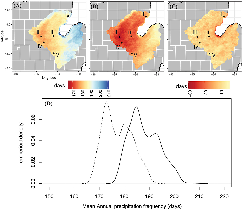
Figure 6. Same as Figure 2, but for mean annual precipitation frequency.

Precipitation intensity is calculated as the mean annual precipitation value at a grid cell divided by the number of days in which precipitation occurs at that location. The average precipitation intensity over the SBW in the historic model run is 4.4 mm/precipitation day while the average intensity in the future model run is 4.8 mm/precipitation day. The model runs have a similar spatial pattern (Figures 7A,B), with the lowest intensities occurring around Saginaw Bay (3.7 mm/precipitation day in the historic model run and 4.2 mm per precipitation day in the future run) and increasing intensities in the northwestern and southeastern parts of the watershed (maximum of 5.1 mm/precipitation day in the historic run and 5.7 mm/precipitation day in the future run). When comparing the average precipitation intensity at each grid cell in the future model run to the historic model run, Figure 7C shows increases in intensity over the twenty-first century with the largest increases of 0.7 mm/precipitation day in the “thumb” region of the Lower Peninsula, the eastern portion of the watershed. This corresponds with the region that saw an increase in total annual precipitation in Figure 6C. The empirical distributions show that in the future time period the average intensity becomes larger and there is less variability within the watershed (as the size of the tails is reduced; Figure 7D). This indicates that by the end of the twenty-first century precipitation in the SBW will become more intense (larger amount per precipitation day) and there will be less variability in the range of intensities experienced.

FIGURE 7

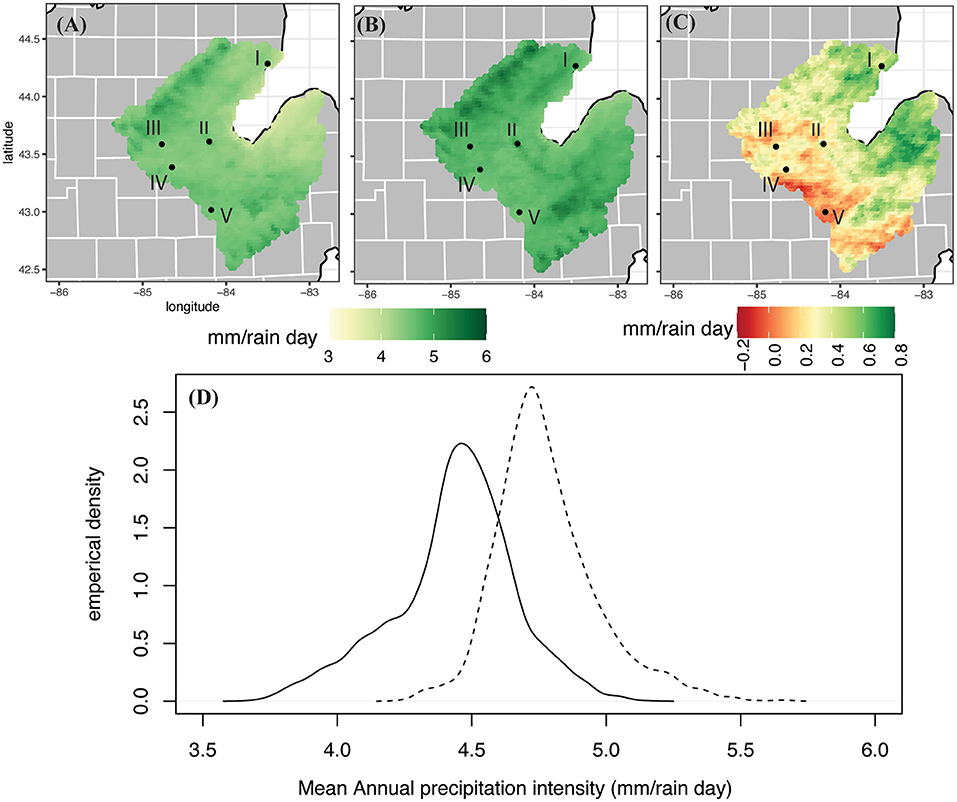
Figure 7. Same as Figure 2, but for mean annual precipitation intensity.

The relative changes in the SBW variables indicate that on average this watershed will warm by 5.7°C in daily maximum temperatures and more (6.3°C) in daily minimum temperatures. Relative humidity shows a slight reducing trend when looking at annual averages. The projected change to total annual precipitation varies across the watershed, but the picture of the characteristics of SBW precipitation is consistent. Precipitation will occur less frequently across the watershed but will be more intense, as the amount that falls per precipitation day will increase. All of the SBW is not projected to have an increase in total annual precipitation because even though all locations are projected to experience increased precipitation intensity, decreases in precipitation frequency also occur across the watershed. In the west and southwestern parts of the watershed the increase in intensity is not enough to negate the decrease in frequency, and the annual total precipitation decreases. Grid cells near the Saginaw Bay coast are expected to experience more extreme changes than the rest of the watershed.

Validation and Bias Correction

WRF Model Validation

For the most accurate one-way coupling of the dynamically downscaled WRF data with a hydrologic model the data must be validated against “ground truth” observations to estimate errors, and bias corrected to compensate for those errors. Since the climate model inputs into SDHMs is spatially explicit both the validation and bias correction are performed at the locations in the SBW that also have in-situ meteorological data for the historic period (1991–2005; Figure 1). For the 5 in-situ weather stations in the study region the average differences between historic modeled data and the historic observations are given in Table 1.

TABLE 1

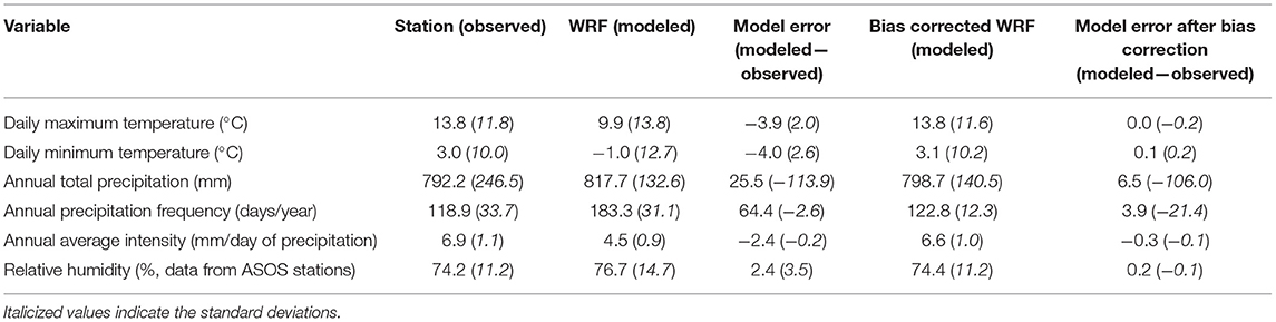
Table 1. Average (standard deviation) of station and WRF variables of interest for hydrologic inputs at the five observational stations within the watershed for 1991–2005.

For daily maximum temperature, the observed mean is warmer than the model output for all stations. The largest difference is 6.5°C, which is located at the north-eastern tip of the SBW. The temperature differences are much smaller near the central part of the lower peninsula [lowest is 2.6°C at Mount Pleasant, MI (station III)]. This indicates that for the SBW region the model keeps the daily maximum temperatures too cool by 3.9°C on average (more near the coast). Standard deviations of the daily maximum temperature show that all station locations have a larger modeled standard deviation than is observed (overall average of 2.0°C larger standard deviation).

The daily minimum temperature shows a similar relationship between modeled and observed values. The largest difference is where modeled temperatures are 6.5°C warmer and again occurs at the East Tawas station, in the north-eastern part of the watershed. Stations in the central part of the MI lower peninsula have smaller differences between the observed minimum temperatures and modeled temperatures, but overall the model generates minimum daily temperatures 4.0°C cooler on average. Differences in standard deviations of minimum temperatures are 2.6°C, indicating that the model produces a larger standard deviation than the observed data. For relative humidity, the WRF model is slightly more moist by 2.4%. It is also more variable, with a standard deviation 3.5% more than observed.

Annual total precipitation (mm) is slightly higher in the historic model run, by 25.5 mm on average. The discrepancy is the highest (765.1 mm observed vs. 861.6 mm modeled) at Midland, MI (station II) in the central part of the lower peninsula, near the western edge of the SBW. The source of this over-production of precipitation in WRF is due to the frequency of precipitation generated in the model. WRF causes precipitation to occur on average 64.4 days too often per year compared to the observed frequency. This is the worst at Mount Pleasant (station III), where the observed frequency is 88.5 days per year and the modeled frequency is 178.7 days per year. On the other hand, the WRF simulation under—produces with regard to precipitation intensity (mm/precipitation day), on average 2.4 mm less than observed [this is larger than the measurement accuracy for human recorded precipitation which is 0.5 mm (NOAA., 2018)]. This difference was also largest at Mount Pleasant, MI (station III) where the average intensity is observed at 9.1 mm/precipitation day and modeled to be 4.5 mm/precipitation day. The combination of too frequent precipitation events but less intense rain events result in close values at Mount Pleasant for total annual precipitation (795.5 mm observed vs. 793.1 mm modeled) although that is because the inaccuracies cancel each other out. This helps to illustrate why adjusting precipitation is still needed, even though errors of total annual precipitation might not seem that high. Accurate capture of precipitation frequency and intensity are particularly important for hydrologic modeling applications. The Kolmogorov-Smirnov test resulted in a p-value is near zero in all cases, indicating that the two distributions are likely not from the same population (p < 0.05) for all stations and all variables. Therefore, bias adjustments are required for the WRF data before ingesting the data into any hydrologic model.

Quantile Mapping Bias Correction

Quantile Mapping bias correction is applied to each of the 5 locations within the SBW that are co-located with in-situ weather stations. The data from the weather stations are used to generate the empirical cumulative distribution function used to transform the WRF historical run data. The transform functions are retained for use at those same locations in future model runs. An example of the results of the bias correction is given in Figure 8, and comparison statistics for all of the variables are shown in Table 1. The Kolomorgov-Smirnov test is again used to determine whether the bias corrected model data is statistically similar to the observed values.

FIGURE 8

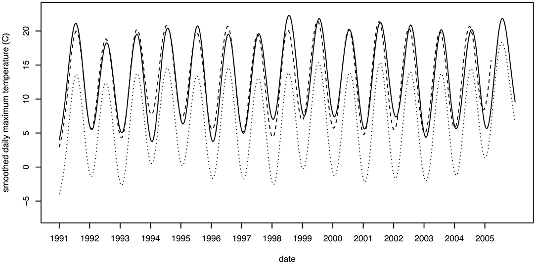
Figure 8. Observed (solid), modeled (dotted), and bias corrected (dashed) modeled daily maximum temperatures for observational station 202423 (Oscoda, MI).

The differences between the bias corrected WRF output and the observational values have been reduced dramatically in Table 1, compared to the un-corrected differences (Model Error column in Table 1). Before, WRF was underpredicting temperatures by 3.9°C (maximum temperatures) and 4.0°C (minimum temperatures). After bias correction, the average difference between modeled maximum temperatures and observed maximum temperatures is 0.0°C, and the average difference for minimum temperatures is 0.1°C. The error associated with the relative humidity also became almost negligible, at a mere 0.2%. A graphical demonstration of the impact of this correction on maximum temperature at the Oscoda, MI location (station I) is shown in Figure 8.

Average annual total precipitation amount observed at the 5 stations is 792.2 mm/year and the un-corrected WRF historic model over-forecasted precipitation by 25.5 mm on average. However, after bias correcting the WRF output, the difference is reduced to 6.5 mm of precipitation per year (Table 1). The intensity of precipitation also shows substantial improvement. Without correction, the WRF model produces precipitation 64.4 more days than observed. After applying the Quantile Mapping bias correction, WRF only generates precipitation 3.8 days per year more than observed. The average intensity of precipitation events was under forecast by WRF by −2.4 mm/day. However, after bias correction this difference is −0.2 mm/day. All three of these variables show the improvements to WRF's ability to represent the nuances of the precipitation regimes after bias correction.

According to the K-S test for the likelihood of two sample distributions coming from the same population, all total precipitation samples (observed, modeled, and bias corrected modeled) are likely from the same population distribution (p ≤ 0.05). This is mostly due to the low error for total annual precipitation values, which we have shown is an artifact of frequency and intensity errors canceling each other out. When considering precipitation frequency and intensity only, the observed and bias-corrected model distributions have statistically significant K-S D values, indicating they are likely from the same distribution (for all 5 stations in the watershed). This is also the case for the other variables, where only after bias-correction could observations and modeled output be assumed to come from the same distribution. The exceptions are with 2 stations failing to meet this assumption at the p ≤ 0.05 significance level for minimum temperature, and one station for maximum temperature.

Bias Corrected Future run

The quantile mapping transforms developed between the station data and historical model data are applied to the 5 corresponding point locations for the RCP 8.5 WRF future run. The resulting values averaged over the 5 locations are given in Table 2 for comparison with the historic model run values. Empirical density functions (edfs) are fit to the historic and future precipitation data in order to estimate the probability distribution functions of the data and to visualize the differences in the entire variable's distribution. The value for the 75th and 90th percentile are computed for precipitation, and the 10th and 90th percentiles for the other variables (Figures 9–12). Above/below average and extreme values can be used to develop relationships between climatological variables and streamflow; this is especially true for precipitation with regards to flood event prediction but also applies temperature and RH for their effects on watershed processes including evapotranspirative demand.

TABLE 2

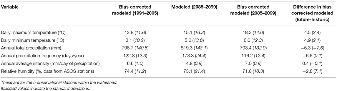
Table 2. Average (standard deviation) of bias corrected WRF variables for the historic and future model runs.

FIGURE 9

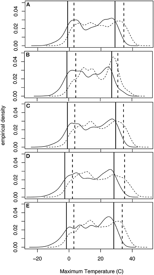
Figure 9. Daily maximum temperature empirical density functions. The solid black line is the historic bias corrected data and the dashed line represents the future bias corrected data at each location. The solid vertical lines represent the 10 and 90% values at location (A) 200146 (Gratiot, IV), (B) 202423 (Oscoda, I), (C) 205434 (Midland, II), (D) 205662 (Mount Pleasant, III) and (E) 206300 (Owosso, V).

FIGURE 10

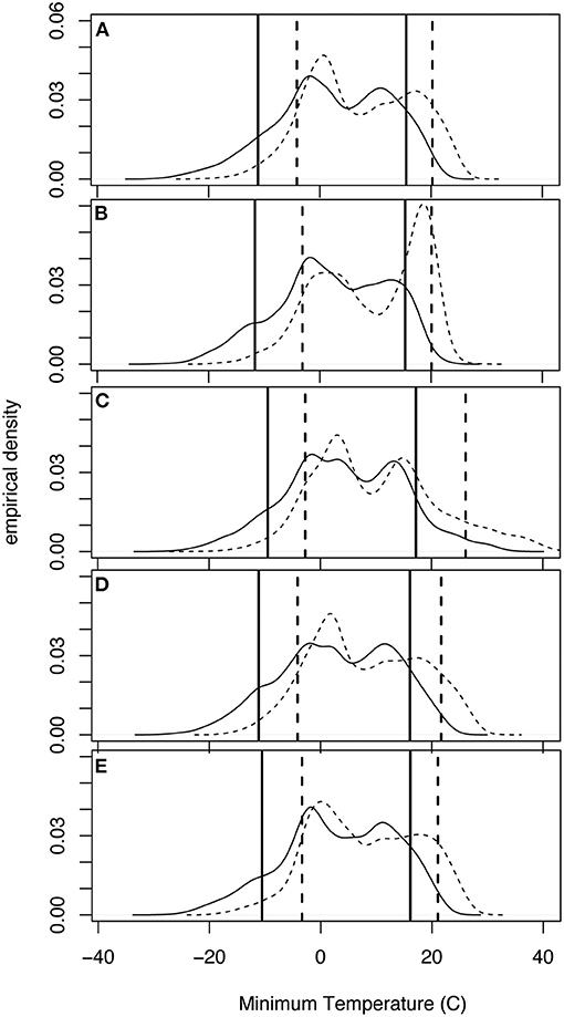
Figure 10. Same as Figure 9 but for daily minimum temperature.

FIGURE 11

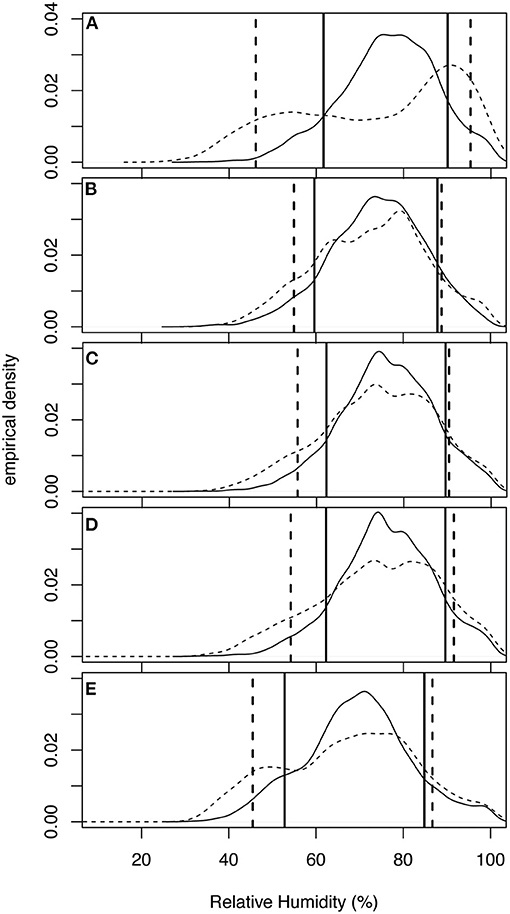
Figure 11. Same as Figure 9 but for daily relative humidity.

FIGURE 12

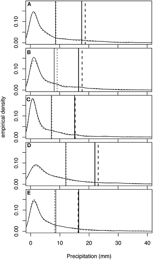
Figure 12. Daily precipitation empirical density functions. The solid black line is the historic bias corrected data and the dashed line represents the future bias corrected data at each location. The dashed vertical lines represent the 75th and 90th (bold) percentile values for the future data and the solid vertical lines represent the 75th and 90th (bold) percentiles values for the historical data at location (A) 200146 (Gratiot, IV), (B) 202423 (Oscoda, I), (C) 205434 (Midland, II), (D) 205662 (Mount Pleasant, III) and (E) 206300 (Owosso, V).

Average daily maximum temperature increases from 13.8 to 18.3°C during the twenty-first century (Table 2). The edfs of maximum temperature calculated for each of the station's historic and future bias corrected variables are displayed in Figure 9. All of the stations experience a shift in the future maximum temperature distributions toward the right, indicating higher temperatures. In addition, the 10th and 90th percentile temperature values increase at all locations with the maximum increase in the 10th percentile of 5.6°C (from −1.1 to 4.5°C) occurring at Oscoda, MI (station I), the northern most location in the SBW (Figure 9B). The largest increase in the size of the 90th percentile temperature is at Mount Pleasant, MI (station III) where the 90th percentile goes from 28.3°C in the historic edf to 35.1°C in the future edf (Figure 9D).

Likewise, the average daily minimum temperatures at the 5 stations within the SBW increase from 3.0 to 8.0°C (Table 2). The edfs of minimum temperatures (Figure 10) show that a shift of the entire distribution toward higher temperatures is consistent across the watershed. It is interesting to note from these comparative distributions that the 10th percentile values increase more than the 90th percentile values at almost all stations, indicating a substantial change in the frequency and value of extreme cold minimum temperatures. The largest of these 10th percentile warmings occurs at Oscoda, MI (station I) in the northern part of the SBW (Figure 10B). The largest warming of the 90th percentile minimum temperature is 8.9°C (from 17.2 to 26.1°C) and occurs at Midland, MI (station II), in the western part of the watershed (Figure 10C).

In the SBW, the future model run produces a signal of decreasing relative humidity from 74.2 to 71.6% (Table 2). Even though the average relative humidity decreases, the average standard deviation of relative humidity increases from 11.2 to 18.3%. This is more easily observed in Figure 11, which plots the historic and future bias corrected edfs of relative humidity at the 5 locations in the SBW. These figures show the flattening of the distribution and the corresponding increase in variability, particularly in the left tail. The 90th percentile values increase at all 5 stations [by as much as 5.3% at Gratiot, MI (station IV); Figure 11A], but the 10th percentiles show the largest amount of change. All of the stations experience a decrease of the 10th percentile values of at least 4.7%, and Gratiot, MI (in the southwestern part of the watershed) experiences a reduction of 15.6% over the twenty-first century. The increased intensity and decreased frequency of precipitation events may lead to longer periods of drier air between events.

Total annual precipitation does not appear to experience substantial change in the future model run once the WRF output is bias corrected (Table 2). There is a slight decrease (−1.2 mm) in average annual precipitation totals at the 5 station locations, due to a decrease in frequency (−2.7 days/year) and increase in intensity (0.1 mm/precipitation day). However, from the spatial maps (Figures 2–7) it can be seen that the projected changes to precipitation vary in magnitude and sign across the watershed, and the bias-corrected future time series are only created at the 5 locations with station data. Figure 12 shows the edfs for the historic and future bias corrected model values for daily precipitation events. For these distributions the 75th and 90th percentiles are indicated on the plots, since understanding above average and extreme precipitation events is paramount for modeling event-based flow. All of the locations experience a slight increase in the magnitude of 75th and 90th percentile events except for Owosso, MI (station V), in the southern part of the watershed (Figure 12E), which corresponds with the area of decreased precipitation intensity in Figure 7C. The largest magnitude increases in 90th percentile precipitation events occur at Gratiot, MI (station IV), Oscoda, MI (station I), and Mount Pleasant, MI (station III; Figures 12A,B,D). These locations experience extreme precipitation increases around 1.2 mm in magnitude and corresponds to areas of increased precipitation intensity in Figure 7C.

Discussion

Inferences and Implications

End-of-century model runs indicate that the SBW will experience substantial and spatially variable effects from climate change. On the whole, the watershed will be slightly drier, with lower relative humidity and fewer precipitation days than at the end of the twentieth century. This change in relative humidity is consistent with what is expected from the Clausius-Clapeyron relation of increased atmospheric moisture capacity without large changes in moisture flux over land (Byrne and O'Gorman, 2016). Temperatures will increase substantially, with the largest changes occurring at the extremes (10th percentile maximum and 90th percentile minimum), meaning that it is likely that the SBW will see simultaneously more frost-free days in the winters and more exceptionally hot days in the summer months. This trend of decreasing diurnal temperature range due to a faster rate of warming by minimum temperatures is consistent with what has happened in the last century (Easterling et al., 1997; Thorne et al., 2016; Sun et al., 2019 among others) and what is expected to continue in a warming climate (Zhou et al., 2009). The small decline in total annual precipitation masks projected increases in precipitation intensity, with the increases in precipitation intensity modeled across nearly the entire watershed. The projected changes will not be uniform, with the coastal region experiencing some of the most extreme temperature changes and considerable spatial variability in precipitation frequency and intensity throughout the watershed. One of the benefits of dynamical downscaling with the WRF model is that finer resolution processes, such as convection, can identify spatial patterns within the study domain that would not be apparent in a coarse-resolution GCM (Qiu et al., 2021). The difference in projected characteristics between the coastal area and inland would have been sub-grid scale in the 1° spatial resolution of the parent climate simulations we used before downscaling, which could also be missed in statistical downscaling without observations to provide “predictand” distributions at those locations. It is important to note that this is on realization of just one GCM-RCM coupling. Other GCMs coupled to other RCMs or multiple realizations of the current GCM-RCM combination would produce different temperature, precipitation, and relative humidity projections. Therefore, the direction and general magnitude of the future projections are more important than the exact magnitude of the changes.

The large increases in mean minimum and maximum temperature along the coast of Saginaw Bay could be a substantial stressor on wetland vegetation; increased air and water temperatures and the associated declines in water level (for emergent wetlands) and water clarity (for submergent wetlands) all can negatively impact wetland plants and potentially decreasing associated ecosystem services including nutrient cycling, sediment trapping and deposition, and flood modulation (Erwin, 2009; Steinman et al., 2012; Junk et al., 2013; Short et al., 2016). Considering the substantial resources that have been committed to restoring coastal wetlands in Saginaw Bay (Hartig et al., 2020), a decline in function due to climate change impacts should be cause for concern. Capturing spatial variability in precipitation frequency and intensity is fundamental to effectively modeling rainfall-runoff ratios, flooding in ungauged catchments, erosion processes, and the potential for mobilization of non-point and point source pollutants. Recognizing that changes in precipitation intensity and frequency will not be uniform and may exacerbate existing watershed stressors like land use change is needed in order to quantify changes in hydrologic regime and prediction of extreme events.

Limitations and Future Work

The distinct difference between the Saginaw Bay coastal grids and the rest of the SBW's projected changes in climate merit future investigation. There are not in-situ stations from the NOAA COOP or ASOS networks within these cells to use for validation, so error cannot be ascertained in the same manner. The closest in-situ station is Oscoda, MI (station I), located along the northern coast of the Saginaw Bay, which had model errors (before bias correction) of less than 0.1 mm for precipitation, ~6% for relative humidity, and ~6.5°C for temperatures. Without further investigation it is unclear if the bias correction applied at Oscoda, MI is appropriate for the rest of the Saginaw Bay coast. Part of the uncertainty here is because the atmospheric model used in this study for dynamical downscaling does not contain a dynamic lake model, but rather designates a “water bodies” land cover type (WRF v3.7; Skamarock et al., 2008), which lacks realistic lake surface temperatures (Gula and Peltier, 2012; Xiao et al., 2016). The study uses a bias-corrected GCM with a nested RCM that was also validated and bias-corrected, which assists in removing some systematic errors that may be introduced because of this inaccurate lake grid treatment. However, research in the last several years has been actively seeking a better coupling between WRF and dynamic lake models for use in regional climate studies (Gu et al., 2015; Xiao et al., 2016; Peltier et al., 2018; Ma et al., 2019; and others). To better understand the reliability of the projections for the Saginaw Bay coastal area, and to what extent bias-correction can remediate a lack of some of the GCM's sub-grid-scale influences, future work may include comparison with some of these lake-coupled models. Additionally, it would be worthwhile to perform the historical downscaling simulation with nudging applied to the RCM, to examine the impact of this “relaxation” toward the GCM on the precipitation variability and extremes over such a fine spatial resolution as the inner domain and over such a long time scale. Another avenue of future work with these data will be to diagnose error and bias-correct all of the modeled grid points within the watershed, for sensitivity analyses with SDHMs. Alternative in-situ observations that are not as long-running as the stations used in this paper or gridded products may be used to supplement the stations within the watershed for these future analyses.

Such high spatial resolution climate data over a long time period processed for coupling with SDHMs is a valuable tool for examining climate change impacts on hydrologic systems. However, the full potential of this dataset is not realized in this study. Even though dynamic downscaling captures the variability in atmospheric processes throughout the watershed, without bias correction of that data before ingestion by hydrologic models errors are needlessly propagated into them and can obfuscate the empirical parameter calibration that must happen. Additionally, questions remain as to how many of the 3 km by 3 km grid cells within the SBW need to be provided as input to a SDHM to capture the necessary atmospheric variability within the watershed, and what is the best method for bias correcting those grid cells without in-situ validation data. Answering these questions will allow future research to more accurately bridge the spatial and temporal gap between GCMs run for future climate scenarios and SDHMs that are able to simulate multifaceted impacts of atmospheric variability on hydrologic processes.

Data Availability Statement

The datasets presented in this study can be found in online repositories. The names of the repository/repositories and accession number(s) can be found below: the dynamically downscaled and bias corrected time series developed for 2085–2099 for the 5 locations can be found at CUASHI's HydroShare (http://www.hydroshare.org/resource/0754e9c2e5a84f90959b2aa9164a4b9e).

Author Contributions

DK and WR contributed to the concept and design of the study. DK performed the dynamical downscaling and climate analysis. Both DK and WR wrote the paper and created the figures. All authors contributed to the article and approved the submitted version.

Conflict of Interest

The authors declare that the research was conducted in the absence of any commercial or financial relationships that could be construed as a potential conflict of interest.

Publisher's Note

All claims expressed in this article are solely those of the authors and do not necessarily represent those of their affiliated organizations, or those of the publisher, the editors and the reviewers. Any product that may be evaluated in this article, or claim that may be made by its manufacturer, is not guaranteed or endorsed by the publisher.

Acknowledgments

The authors would like to thank Lucas Falsetta for technical assistance with the WRF setup at CMU and to the editors and reviewers for their suggestions to improve the manuscript.

Footnotes

1. ^https://rda.ucar.edu/datasets/ds316.1.

References

Alexandru, A., de Elia, R., Laprise, R., Separovic, L., and Biner, S. (2009). Sensitivity study of regional climate model simulations to large-scale nudging parameters. Monthly Weather Rev. 137, 1666–1686. doi: 10.1175/2008MWR2620.1