 Fengyi Xie
 Andre R. Erler2
 Deepak Chandan
- 1Department of Physics, University of Toronto, Toronto, ON, Canada
- 2Aquanty, Waterloo, ON, Canada
Extreme heat events in the Great Lakes Basin (GLB) region of eastern North America are expected to increase in concert with greenhouse gas (GHG) induced global warming. The extent of this regional increase is also influenced by the direct effects of the Great Lakes themselves. This paper describes results from an ensemble of dynamically downscaled global warming projection using the Weather Research and Forecast (WRF) regional climate model coupled to the Freshwater Lake (FLake) model over the Great Lakes region. In our downscaling pipeline, we explore two sets of WRF physics configurations, with the initial and boundary conditions provided by four different fully coupled Global Climate Models (GCMs). Three time periods are investigated, namely an instrumental period (1979–1989) that is employed for validation, and a mid-century (2050–2060) and an end-century (2085–2100) periods that are used to understand the future impacts of global warming. Results from the instrumental period are characterized by large variations in climate states between the ensemble members, which is attributed to differences in both GCM forcing and WRF physics configuration. Results for the future periods, however, are such that the regional model results have good agreement with GCM results insofar as the rise of average temperature with GHG is concerned. Analysis of extreme heat events suggests that the occurrence rate of such events increase steadily with rising temperature, and that the Great Lakes exert strong lake effect influence on extreme heat events in this region.
1. Introduction
Record breaking extreme heat events have been occurring more frequently around the world in recent years. Some, such as the extreme heat events over Europe in 2019 (Vautard et al., 2020) and over western North America in 2021 (Philip et al., 2021) were especially severe, causing significant loss of life and property. This trend of increasingly active heat events has attracted a great deal of attention from the public, businesses and policy makers. Interest is particularly great in attempting to understand the susceptibility of regions of interest, such as those at high risk of wildfires to changes in the frequency of these events.
The Great Lakes Basin (GLB) region of North America is the largest fresh-water system on Earth, by area, and supports a population in the tens of millions along with extensive agricultural and industrial activity. Extreme heat events can be very debilitating to this region, and lead to impacts that would be felt far-and-away. It is therefore of great interest to understand climate change induced changes to extreme heat events and the extent to which the influence of such events may be affected by the presence of the Great Lakes. The purpose of the present paper is to begin a discussion on the expected frequency of occurrence of extreme heat events in the GLB in the future.
The climate of the GLB has traditionally been studied from either an observational perspective (Scott and Huff, 1996) or via the application of coupled Global Climate Models (GCMs; Lofgren, 1997). In recent years, however, there have been advances in the usage of high-resolution Regional Climate Models (RCMs), often in conjunction with a lake model, to study the impacts of global warming in this region at a resolution and fidelity higher than that which is afforded by GCMs.
The first attempt to examine the GLB region with an RCM together with a lake model was undertaken by Gula and Peltier (2012) who employed WRF in a dynamical downscaling pipeline wherein the NCAR CCSM3 global model (Collins et al., 2006) was used to force a nested WRF configuration with an outer domain covering the entire North American continent at 30 km resolution and an inner domain covering the GLB at 10 km resolution. The lake model in their study, FLake (Mironov, 2008), was run in offline mode, nevertheless, it was apparent from the study that FLake was able to accurately represent the area covered by lake ice in winter as well as the timing of onset and retreat of the lake ice. More importantly, the analysis demonstrated the capability of nested dynamical downscaling to fully resolve lake effect meteorological processes such the formation of snow belts in the lee of the lakes during winter, and to describe the impacts of the global warming in that region.
The nested downscaling pipeline of Gula and Peltier (2012) was enhanced further by fully coupling FLake to WRF and the improved configuration was used by d'Orgeville et al. (2014) to present the first study of the expected changes to extreme precipitation in the GLB under the influence of anthropogenic climate change. High resolution output from the inner WRF domain was employed to drive an analysis of precipitation extremes using a peak-over-threshold technique to quantitatively assess the extent to which the return times of extreme precipitation events of varying intensities are expected to decrease through the current century under the RCP8.5 “business as usual” radiative forcing scenario. It was found that the time separating extremes of any given precipitation intensity would decrease by at least a factor of two by mid-century. A follow up study by Peltier et al. (2018) made use of a larger ensemble of WRF physics configurations and investigated the “fattening of the tail” of the probability distribution under climate change by using the Generalized Extreme Values (GEV) distribution methodology. The results for end-century for both temperature and precipitation were in agreement with the earlier analyses of d'Orgeville et al. (2014).
Following Gula and Peltier (2012), results from the application of RCMs to the understanding of the climate of the GLB started to be reported by other researcher groups. Notaro et al. (2013) reported on an RCM configuration that employed the Abdus Salam International Center for Theoretical Physics Regional Climate Model, version 4 (ICTP RegCM4), forced by the National Centers for Environmental Prediction (NCEP)–NCAR reanalysis and the Global Sea Ice and Sea Surface Temperature (GISST) dataset from the UK Met Office, coupled to a one-dimensional energy-balance lake model. By comparing their results for the GLB with those obtained from another model run in which the lakes were replaced by a landscape similar to that of the surrounding region, they demonstrated that the presence of the Great Lakes reduces the amplitude of both diurnal and annual temperature change due to their large thermal inertia. Subsequently, Notaro et al. (2015b) forced their lake coupled RegCM4 model with the outputs of two Coupled Model Intercomparison Project Phase 5 (CMIP5) GCMs over the historical and future global warming periods. The results demonstrated, unsurprisingly, that winter temperature is expected to rise, and that reduced lake ice cover leads to an increase in lake effect precipitation which gradually shifts from snow to rain as the climate continues to warm. In an accompanying paper, Notaro et al. (2015a) discuss the effect of projected changes in precipitation and evaporation on future lake levels.
Mallard et al. (2014) also employed WRF coupled to the FLake model and showed that the configuration is able to simulate the regional climate with higher accuracy than reanalysis that has a lower spatial resolution. Xue et al. (2017) coupled RegCM4 with a different lake model based on the Finite Volume Community Ocean Model (FVCOM) 3D hydrodynamic model to obtain highly accurate lake fields. Recently, by coupling the NASA-Unified WRF model (NU-WRF) to both a 1D lake model and a 3D lake model, Notaro et al. (2021) showed that the 3D lake model performed better over the Great Lakes region.
A major shortcoming in this extensive literature on the application of RCMs to the GLB is that nearly all of these studies used global forcing data from only one GCM. Therefore, the effect of the choice of GCM data on the downscaled results for the GLB remains largely unconstrained. Zobel et al. (2018b) presented regional climate results over the Continent of US (CONUS) from the WRF model forced by 3 different GCMs and demonstrated that different GCM forcings lead to significant differences over their domain. Therefore, we could expect to see a similar variability in the downscaled climate over the GLB region depending on the GCM data. Here we make progress on filling this knowledge gap by using outputs from a selected set of GCMs that have participated in the Coupled Model Intercomparison Project Phase Five (CMIP5; Taylor et al., 2012) and whose data have been uploaded to the project archive. The CMIP5 models have been used to simulate both the twentieth century over which their results can be verified against high quality instrumental observations, and the twenty-first century over which we are interested in performing downscaled projections. The CMIP5 archive was key to the findings reported in the IPCC Fifth Assessment Report (IPCC, 2013a) and the data has been used for understanding climate change projections over North America (Sheffield et al., 2013a,b).
In addition to the mean climate state of the GLB region, the modeling of extreme events and projections of their change into the future has also generated considerable interest. Modeling and projection of changes in extreme precipitation using a lake model coupled to a RCM has been previously reported (d'Orgeville et al., 2014; Peltier et al., 2018), but in contrast much less effort has been expended to studying extreme heat events using this configuration. While some studies have attended to the question of regional extreme heat events, those have been either based on observations (Peterson et al., 2008) and so cannot be used for future projections, or use low-resolution GCM data (Meehl and Tebaldi, 2004; Kharin et al., 2013; Sillmann et al., 2013a,b) or downscale GCM data without resolving lake dynamics (Jeong et al., 2016; Byun and Hamlet, 2018). The latter two approaches are unable to explicitly include lake effects in the Great Lakes region. Studies have shown that lakes are not immune to climate change (O'Reilly et al., 2015; Woolway et al., 2020), and therefore interaction between a warmed lake and its surroundings needs to be resolved by a lake model in order to obtain accurate climate change signal over the surrounding region.
This study will employ the dynamical downscaling pipeline that was recently used in Peltier et al. (2018) but apply it to CMIP5 data to construct a new ensemble of downscaled simulations. This new ensemble will be used to explore the variability in the downscaling process when forcing from different GCM models is employed, and thereby attempt to address the impact of GCM selection on regional climate results. Extreme heat event analysis is performed on this ensemble to explore the evolution of heat waves under the influence of different simulations for climate change.
2. Experimental Design, Climate Models, and Validation Datasets
2.1. Experimental Design
The dynamical downscaling experiments presented in this paper follow the two-step nesting procedure established in Gula and Peltier (2012) and d'Orgeville et al. (2014) wherein the first of the nested domains, namely the outer domain, covers the continent of North America at a resolution of 30 km, and the nested inner domain covers the GLB at 10 km resolution. Technical details are described in Erler (2015). This pipeline has also been employed to perform downscaling experiments in other regions, such as Western Canada (Erler et al., 2015; Erler and Peltier, 2016, 2017), and India and South-east Asia (Huo and Peltier, 2019; Huo et al., 2021).
2.2. CMIP5 GCM Models
The CMIP5 archive contains data generated by over 50 climate models from 20 modeling groups from around the world. It is a comprehensive source of global climate data for both historical and future projection periods (Taylor et al., 2012). Several studies have used the CMIP5 archive to investigate future climate projections over various regions of the world (see for example Kug et al., 2015; Song and Yu, 2015; Cheng et al., 2017; Peings et al., 2017), and the relative performance of the models, over North America has been evaluated for the historical period (Kumar et al., 2013; Sheffield et al., 2013a,b) and the future (Maloney et al., 2014).
Our downscaling pipeline requires the availability of several atmospheric, sea ice and land surface variables from the GCM at 6-h resolution. At the time of this study, only data from MIROC5, GFDL-ESM2M and GFDL-CM3 stored on the CMIP5 archive satisfied these requirements. Accordingly, in this study we use data from these three GCMs, together with data from our own simulation using CESM1. Sheffield et al. (2013a) found that these models cover a broad range of performance and concluded that CESM1 is one of the better performing models, while GFDL-CM3 is among the models that perform worse over the historical period. Both GFDL-ESM2M and MIROC5 were ranked in between CESM1 and GFDL-CM3. We therefore expect this set of models to provide a good spread of climate states in the RCM ensemble.
The Model for Interdisciplinary Research on Climate (MIROC; Watanabe et al., 2010) is developed and operated by the Japanese research community. The atmospheric component of the model has a spectral dynamical core that operates at a horizontal resolution of T85 (1.4° × 1.4°) and has 40 layers in the vertical. The ocean grid uses stereographic projection and conformal mapping to transfer the north pole to 80°N, 40°W and the south pole to 80°S, 40°W in order to prevent the geometric singularity due to the convergence of the meridians from existing in the oceanic domain. The grid resolution in the zonal direction is fixed at 1.4° but the meridional resolution decreases from 0.5° at 8° equivalent latitude to 1.4° at equivalent latitudes poleward of 65°. The vertical discretization includes 49 layers that are unevenly distributed with greater concentration near the surface. The atmospheric component uses parametrization schemes that includes a cumulus convection scheme, cloud and cloud microphysics schemes, turbulence diffusion scheme and an aerosol model. Sea ice is treated on ocean cells with dynamics and thermodynamics included. The land component operates with 6 soil layers and includes snow and ice albedo effects, and a lake submodel.
The Global Coupled Carbon–Climate Earth System Model (GFDL-ESM2M) is developed by the Geophysical Fluid Dynamics Laboratory (GFDL) of the National Oceanic and Atmospheric Administration (NOAA; Dunne et al., 2012, 2013). This model uses a finite volume dynamical coreon an atmospheric grid with 2.5° longitude and 2.0° latitude horizontal resolution and 24 vertical levels. The tripolar ocean grid has a horizontal grid spacing of 1° that gradually decreases to 1/3° meridionally at the equator and has 50 vertical levels. The land model parameterizes all physical and biological processes and the included carbon cycle simulates carbon transport between the model components. Components that treat sea ice and icebergs are also included in the model.
The GFDL Global Coupled Model (GFDL-CM3 Donner et al., 2011; Griffies et al., 2011) is also from GFDL. This model uses a finite-volume dynamical core with a cube-sphere grid that has 48 vertical levels and 48 cells along each edge of the cube, leading to grid cell sizes that range from 163 km to 231 km. The output data of this model are projected to an atmospheric grid with 2.5° longitude × 2.0° latitude resolution. This model includes the same ocean and land model components as GFDL-ESM2M. This model also employed various parametrization schemes including aerosol physics, cloud physics, and schemes for trace gas and ozone.
Using multi-millennial runs performed with the two GFDL models, Paynter et al. (2018) show that GFDL-CM3 model has a higher equilibrium climate sensitivity than GFDL-ESM2M. Furthermore, Maloney et al. (2014) show that the GFDL-CM3 model experiences more warming compared to other models in the CMIP5 archive at the end of the twenty-first century. Therefore, we expect the GFDL-CM3 forced RCM experiments to be warmer than other members during the future projection periods.
The fourth member of our ensemble is driven by the Community Earth System Model version 1 (CESM1; Gent et al., 2011), which has been used in previous studies from the Toronto group. CESM1 is a fully coupled global climate model developed by the National Center for Atmospheric Research (NCAR) and contains submodels for all major components of the climate system. The atmospheric component, called CAM4, (Neale et al., 2013) operates on a latitude-longitude grid with resolution 1.26° × 0.9° and 26 vertical layers. The ocean component, called the Parallel Ocean Program (POP) version 2 (Danabasoglu et al., 2012), uses a displaced-dipole grid with 1° longitudinal resolution, varying latitudinal resolution from 0.27° near the equator to 0.54° near the pole and has 60 vertical level. The land component, Community Land Model version 4 (CLM4 Lawrence et al., 2012), runs on the same grid as the atmospheric component and has 15 soil layers. The sea ice component is the Community Ice Code version 4 (CICE Holland et al., 2012) that runs on the ocean grid and simulates both dynamics and thermodynamics.
The CESM1 data used in this study (and in other studies from this group) is from a local simulation performed with the model and therefore there will be subtle differences between this data and that on the CMIP5 archive. Peings et al. (2017) examined internal variability in a large ensemble of 40 CESM1 simulations and concluded that the model does not display significant internal variability. Therefore, using a local CESM1 simulation as forcing should not affect its reliability and the results can still remain comparable to those obtained using CESM1 data from the CMIP5 archive. Previous studies have thoroughly discussed the behavior of CESM1 forced dynamical downscaling experiments (d'Orgeville et al., 2014; Li et al., 2018; Peltier et al., 2018; Zobel et al., 2018b) with most of the studies concluding that CESM1 forced climate results match observations closely. Henceforth, to distinguish between the models whose data were directly obtained from the CMIP5 archive and CESM1 for which we use local data, we will use the phrase CMIP5 models to refer to the collection of GFDL-CM3, GFDL-ESM2M and MIROC5, and the term CMIP5 data as data for these three models. These terms will not refer to the CESM1 GCM or data from that model.
The representation of lakes in the GCMs and their performance deserve attention since we are interested in the GLB region. All GCMs that we employ in this study contain a lake submodel within the land component. However, given the resolution of the GCMs (1° for CESM, T85 for MIROC5, and 2° for the GFDL models), the representation of lakes is very coarse and they are often defined in terms of fractional units of land grid cells. This leads to a poor representation of lake extents and of land-lake contrast. As a result, those lake models cannot represent lake effects in a manner that is achievable when using a high-resolution lake model within an RCM (Notaro et al., 2013). Briley et al. (2021) analyzed how CMIP5 models simulate the Great Lakes and concluded that representation to not be very credible.
Each GCM is forced by historical greenhouse gas concentrations for the historical period (pre-industrial to 2005) and by Representative Concentration Pathway 8.5 (RCP8.5) emissions scenario from year 2006 to year 2100.
2.3. RCM Model Configuration
The regional climate model employed for this study consists of the Weather Research and Forecasting (WRF) model, version V3.4.1, with the Advanced Research WRF (ARW) dynamical core (Skamarock and Klemp, 2008), fully coupled to the Freshwater Lake (FLake; Mironov, 2008) model. The FLake model is configured with a 70 m false bottom as in d'Orgeville et al. (2014) and Peltier et al. (2018). In these two studies, five different sets of physics configurations were employed and discussed, and here two of the sets, namely G and T (see Table 1 of Peltier et al., 2018, for details of the two sets), will be used so that variations in modeled result caused by differences in GCM forcing data could be cross compared with variations caused by different physics configuration sets. The T physics set use the WRF single-moment 6-class microphysics (Hong and Lim, 2006) and the Kain-Fritsch cumulus parameterization (Kain, 2004) schemes while the G physics set uses the Morrison microphysics scheme (Morrison et al., 2009) and the Grell-3 cumulus scheme (Grell and Dévényi, 2002). Other configurations, which are common to both sets, include the Noah land surface model (Chen and Dudhia, 2001), the Rapid Radiative Transfer Model for General Circulation Models (Iacono et al., 2008) radiation scheme and the Mellor-Yamada-Nakanishi-Niino level-2.5 (Nakanishi and Niino, 2009) planetary boundary layer parameterization scheme.
The dynamical downscaling process follows the procedure established in Gula and Peltier (2012), wherein forcing in the from of large-scale GCM data is used as initial condition and boundary condition for WRF. The boundary forcing data includes 6-h temperature, wind, humidity and pressure, whereas the initial conditions include land surface temperature, sea surface temperature, sea ice cover and assorted variables required for the initialization of the land component. A relaxation zone is used to apply boundary forcing smoothly into the WRF outer domain. Spectral nudging is also applied to the pressure, wind, potential temperature and humidity fields in the outermost domain in all ensemble members in order to preserve the large-scale circulation features of the GCMs. For each ensemble member, we perform experiments for three different time periods: historical (1979–1989), mid-twenty-first century (2050–2060), and end-twenty-first century (2085–2100). The WRF simulations also employ the RCP8.5 emission scenario, so the strength of anthropogenic forcing is kept the same as in the GCMs. Lake data is not used to force WRF runs in this study, so the WRF results presented here are not affected by the lake representation in GCMs.
2.4. Validation Datasets
To validate simulations for the historical period, observational and reanalysis datasets are employed. The Natural Resource Canada (NRCan; McKenney et al., 2011) observational data is used to provide ground truth for surface temperature, precipitation, and incoming shortwave radiation. It should be noted explicitly that the NRCan dataset does not have direct measurements over the lakes, so surface temperatures over the lakes are interpolated from nearby land stations and therefore might deviate from true values. The Climate Forecast System Reanalysis dataset (CFSR; Saha et al., 2010) is used to compare surface pressure fields.
Throughout the paper, summer includes the months June, July, and August while winter includes December, January and February. Unless otherwise stated, model results presented are averaged over all years in the respective time periods.
2.5. Methods and Data Used for Extreme Heat Event Analysis
Before performing any analysis of extreme heat events, it is necessary to fix a working definition for such extremes. Several definitions have been proposed and used in the literature and studies have found that the detected heat events are sensitive to the choice of definition (Robinson, 2001; Perkins and Alexander, 2013). It has also been suggested that the definition of a heat event should be customized to suit the climate of the region of interest. For this study, this requires being cognizant of the lake effects that would be accurately simulated by our setup which includes a lake model. During summertime the lakes reduce the maximum atmospheric temperature achievable by absorbing heat, resulting in a cool zone around the lakes (Scott and Huff, 1996). This cooling effect will dampen the tail end of the distribution of extreme heat events extracted by percentile thresholds, so a static threshold method is preferred. For this reason, we choose the Environmental and Climate Change Canada's definition of a heat wave as ‘a period with more than three consecutive days of maximum temperatures at or above 32°C/90°F’ in this study.
At the same time, the lakes also serve as a source of moisture during the summer season. Although the evaporation process absorbs heat and moderates the temperature, the increase in relative humidity itself increases the risk to the health of the inhabitants of the region. Therefore, here we also use the Heat Index (HI) method from NOAA/National Weather Service (Anderson et al., 2013) which combines temperature and relative humidity into a single index (Appendix A1). There are several other widely used measures that also seek to combine temperature and humidity, including Environmental and Climate Change Canada's Humidex, (https://www.canada.ca/en/environment-climate-change/services/sky-watchers/glossary.html) and the wet bulb globe temperature (Li et al., 2017). Exploring their differences is beyond the scope of this study.
Calculating HI requires both temperature and relative humidity which are provided on daily interval by WRF. Days in each model year that experience extreme heat events are determined using the HI definition above (similarly extreme heat days are identified using temperature only when using the temperature metric). The threshold values for the definition of heat waves is kept the same in both the temperature and HI methods, and for all time periods without any bias correction. Original GCM output is not included in this analysis for two reasons: firstly, as discussed above none of the GCMs include a lake model that can suitably capture lake effect and secondly, extreme heat event analysis with GCMs has already been covered by other studies (e.g., Kharin et al., 2013; Sillmann et al., 2013a,b).
3. Mean Climate and Extreme Heat Event Analysis from Dynamical Downscaling
3.1. Simulation Results Over the Historical Period
The winter average near surface temperature (T2) biases with respect to the NRCan dataset (henceforth bias is defined as model minus observation) over the outermost WRF domain are presented for the selected GCM results and the GCM driven downscaled results in Figure 1. It is readily apparent that the downscaled experiments are producing results that are distinctly different from the GCM data that is used as their forcing. This is particularly the case for WRF simulations forced with CMIP5 models, whereas WRF results forced with CESM1 show the smallest (but still sizeable) differences with the GCM data. The strongest biases in CESM1 are the warm bias over Alaska and northeastern Canada and the cold bias over northern Canada. These features are retained to varying degrees in the downscaled experiments, with the G physics version greatly attenuating the cold bias without effecting the warm bias and the T physics version being successful in reducing the magnitude of both biases. On the other hand, while the G physics version is able to improve the performance by attenuating the moderate warm bias throughout the interior of the continent, the T physics version replaces that with a moderate cold bias.
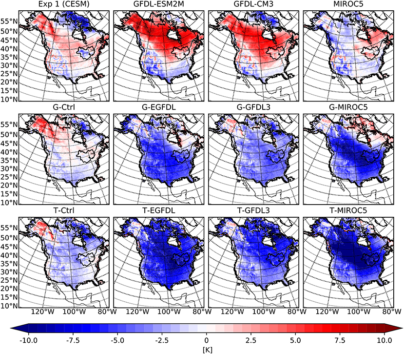
Figure 1. Mean winter season 2 m air temperature biases with respect to the NRCan dataset over the outer WRF domain for the GCMs (top row), WRF ensemble members with G physics (middle row), and WRF ensemble members with T physics (bottom row). From left to right are experiments (GCM or GCM driven WRF) associated with CESM1, GFDL-ESM2M, GFDL-CM3 and MIROC5 respectively.
The MIROC5 model does not have a strong bias over North America, but the two GFDL models produce strong warm bias over Canada, Alaska and northwestern US. In contrast, the WRF results associated with these models all have a large cold bias over the continent, up to 5°C in most regions and up to 10°C in the coldest regions. The magnitude of this bias is larger than the natural variability in the models for this region as previous studies (d'Orgeville et al., 2014; Peltier et al., 2018) have shown that the typical range of bias with physics or initial condition ensemble is ~4°C. This range is also applicable for other regions such as western Canada (Erler and Peltier, 2017), India (Huo and Peltier, 2019), and North America (Zobel et al., 2018b), and is in general also true for other models (for a discussion of variability in GCM results, see Deser et al., 2012, 2014; Peings et al., 2017).
The source of this large cold bias in WRF results with CMIP5 models can be traced to the large-scale wind and pressure fields, and the jet stream position. We begin with an examination of the jet stream position first. The left panel of Figure 2 reveals that in WRF there is a 10° difference in the position of the jet stream between CESM1 forced and CMIP5 forced results. This bias in jet stream position is inherited from CMIP5 forcing data through the spectral nudging process. In order to give a reasonable ground state as reference, the zonal wind from ERA-Interim reanalysis data (Dee et al., 2011) is also plotted, and the ERA-Interim results lie right between the northward biased CESM1 and southward biased CMIP5 results. Since the position of the sub-tropical jet stream marks the northern extent of the Hadley Cell, a southward shift in the position of the jet stream means that heat transport from the tropics by the Hadley cell terminates further southward. This leaves the region north of the jet stream under the influence of colder polar air from the Arctic instead, which disrupts surface temperature fields in the WRF. Furthermore, the largest cold bias in each of the CMIP5 forced WRF results is centered in the range 40° N to 50° N, which overlaps with the region where a shift in the jet stream position would be most influential.
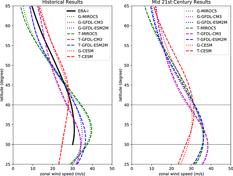
Figure 2. Winter season zonally mean zonal wind speed at 250 hPa pressure level. Left panel shows results for the historical period where ERA-Interim reanalysis result is plotted in black as reference, and the right panel shows result for mid-century period. 30°and 40°latitude are marked to enable easier comparison between plotted curves.
The second cause for the bias in CMIP5 driven WRF results is the surface pressure field. Figure 3 displays the bias of winter season average mean sea level pressure over the WRF outer domain. It is to be noted that the bias in the pressure fields for each GCM differ considerably as a function of increasing latitude: CESM1 varies from high to low, GFDL-CM3 is low over land and high over the Arctic Ocean, and both GFDL-ESM2M and MIROC5 vary from low to high. Since air flows outwards from high-pressure region, a high pressure bias over high latitude forces cold polar air southward thereby causing surface temperatures to drop. As a result, downscaled simulations forced by MIROC5 and GFDL-ESM2M have the largest surface cold bias while GFDL-CM3 forced results have a smaller cold bias and CESM forced results have almost no cold bias.
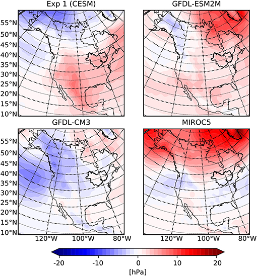
Figure 3. Winter season sea level pressure biases with respect to the CFSR dataset for the GCMs over the WRF model outer domain.
As discussed in Scott and Huff (1996), the Great Lakes moderate air temperature above them by absorbing heat from air during spring-summer season, and releasing it back during the fall-winter season. The release of heat continues until lake surfaces are completely frozen and thermal exchange between lake surface and the atmosphere is blocked. These lake characteristics are confirmed by previous work that employed RCMs coupled to lake models (Gula and Peltier, 2012; Notaro et al., 2013; Mallard et al., 2014). A closer look at winter average near surface temperature (T2) biases over the WRF inner domain (Figure 4) reveals that the cold biases over the lake surfaces and the surrounding regions is smaller by ~2°C than biases over other regions in both CESM and CMIP5 members of the ensemble. This demonstrates that the lake model employed in this study is effective at resolving the temperature mitigating effects of the presence of the lakes even when the region is dominated by a large cold bias. In contrast, in GCM results regions over the lakes are colder than their surroundings, which is contrary to what is expected. This supports the findings of Briley et al. (2021) who found that GCMs do not simulate lake effects accurately because they do not contain a detailed lake model that explicitly resolves land-atmosphere-lake coupling and the exchange of fluxes between them. Figure 5 shows the precipitation bias over the inner WRF domain for all ensemble members in winter, and again the WRF results are able to better capture the spatial distribution compared to their GCM counterparts. Although a smaller bias still exists in regions around the lakes where the lake effect matters, it is likely caused by the cold temperature bias that freezes the lakes early and suppresses evaporation, thereby reducing overall moisture source for those regions.
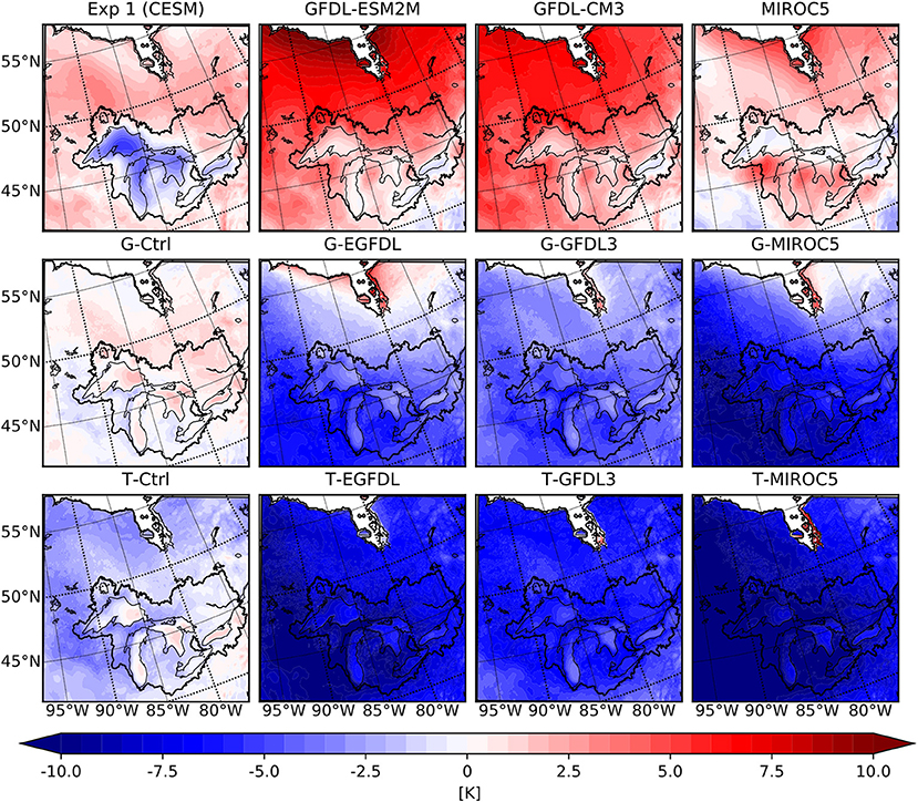
Figure 4. Mean winter season 2 m air temperature biases with respect to the NRCan dataset over the inner WRF domain for the GCMs (top row), WRF ensemble members with G physics (middle row), and WRF ensemble members with T physics (bottom row). From left to right are experiments (GCM or GCM driven WRF) associated with CESM1, GFDL-ESM2M, GFDL-CM3 and MIROC5 respectively. The Great Lakes basin is outlined in black.
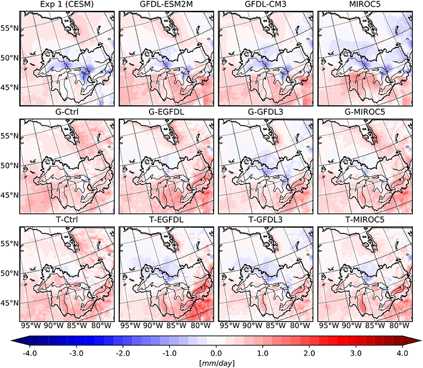
Figure 5. Similar to Figure 4 but for the mean winter precipitation differences.
The near surface temperature (T2) averaged over the summer season for all ensemble members and their respective GCMs are compared with the NRCan dataset over the outermost WRF domain in Figure 6. There is a noticeable difference between the G physics and T physics ensemble members; the latter are warmer than the former by ~2 °C. In Figure 7 the bias in the incoming shortwave radiation for all ensemble members during the summer season is displayed, and it is immediately clear that the primary discriminant in modeled results for this variable is the choice of parameterization set. This difference in surface incoming shortwave radiation is very likely caused by different cloud cover fractions in the atmosphere, which is determined by cumulus and microphysics schemes. These schemes affect cloud cover and cloud reflectance, thereby modifying the planetary albedo. The difference in incoming shortwave radiation also explains why simulations using G physics have a colder surface than those using T physics, which is consistent with earlier results reported in d'Orgeville et al. (2014), and Peltier et al. (2018) that different physics schemes lead to different bias in WRF results. For more information on the impact of physics schemes in atmospheric modelling, see Thompson et al. (2016) who examined the impact of cloud physics and radiation parametrization on WRF simulations, and also Fouquart et al. (1990) for general information on the influence of clouds on radiation in climate modelling.
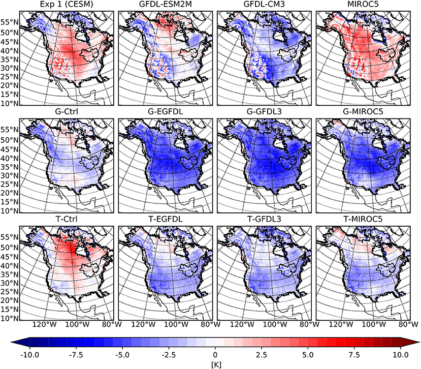
Figure 6. Mean summer season 2 m air temperature biases with respect to the NRCan dataset over the outer WRF domain for the GCMs (top row), WRF ensemble members with G physics (middle row), and WRF ensemble members with T physics (bottom row). From left to right are experiments (GCM or GCM driven WRF) associated with CESM1, GFDL-ESM2M, GFDL-CM3, and MIROC5, respectively.
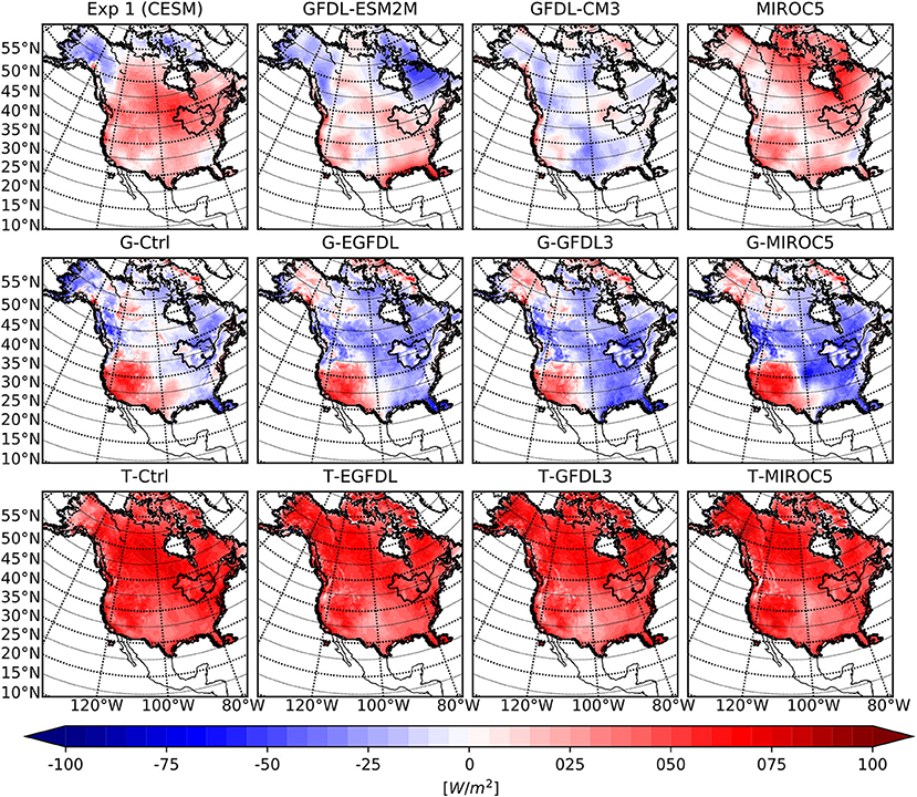
Figure 7. Similar to Figure 6 but for the incoming shortwave radiation differences.
In summer, the CESM1 driven WRF result is ~2°C warmer than CMIP5 driven results, which is caused by differences in GCM forcing data. The jet streams are weaker and meridional pressure gradients are flatter in summer, thus the GCM caused cold bias is smaller in magnitude than in the winter season. Meanwhile in Gula and Peltier (2012) a 2–3°C temperature difference in the region around the lakes is also reported due to the inclusion of the lake model, which is of similar magnitude as biases from other causes discussed herein. Therefore, lake effect is a first order influence on the regional climate and we again confirm the findings in Bates et al. (1993), Lofgren (1997), Notaro et al. (2013) and Mallard et al. (2014) that including a proper lake model is absolutely necessary to properly resolve climate around the lakes.
Choice of physical parameterizations also has a strong influence on the modeled precipitation. The precipitation bias for the same collection of model results is presented in Figure 8 for the winter season and in Figure 9 for the summer season. For both season the primary difference in spatial pattern is between the group of WRF members using G physics and the group using T physics, stronger in summer season as there is little precipitation over winter, and little to no difference across members driven by different GCMs. Related works (d'Orgeville et al., 2014; Huo and Peltier, 2019) also revealed that different sets of physical parameterizations would create large differences in the precipitation result. Note that none of the WRF results have a spatial pattern that resembles the pattern of their respective GCM forcing data, so precipitation data from GCMs is rewritten by the RCM model over the regional domain. Results from (Zobel et al., 2018a) also show that precipitation from RCMs are completely different from GCMs that are used for forcing, indicating that model settings used in the RCM exert a strong influence over modeled precipitation.
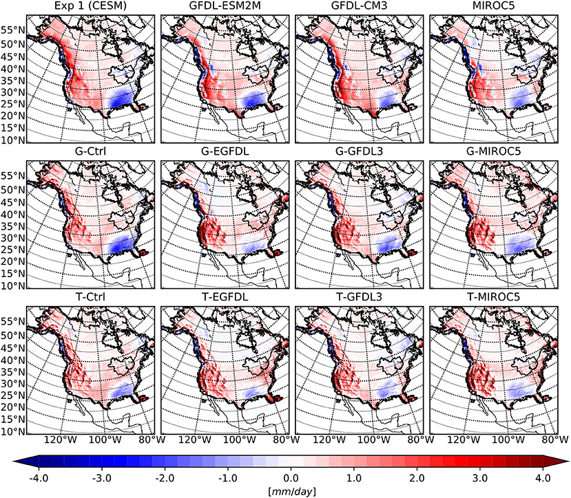
Figure 8. Mean winter season precipitation biases with respect to the NRCan dataset over the outer WRF domain for the GCMs (top row), WRF ensemble members with G physics (middle row), and WRF ensemble members with T physics (bottom row). From left to right are experiments (GCM or GCM driven WRF) associated with CESM1, GFDL-ESM2M, GFDL-CM3, and MIROC5, respectively.
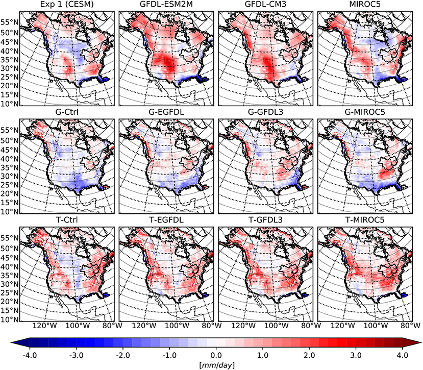
Figure 9. Same as Figure 8 but for summer precipitation biases.
3.2. Simulation Results Over Future Projection Periods
Before presenting climate results for the two climate projection periods discussed in section 2, several technical details need to be stated here. First, all comparisons of CMIP5 ensemble member for future projection period results have been performed with respect to the historical results of each individual ensemble member. Second, in order to preserve the model variability signal, no bias correction has been applied before comparing model results. Third, the two future projection periods (the mid-century (2050–2060) and the end-century (2085–2100) periods) have different time length, but results of the two periods will still be presented in the form of averages over all years over each time period.
According to conclusions in section 3.1, jet stream position has the potential to inflict large temperature bias in the RCM results. Therefore, changes in jet stream position during future projection periods should be examined to determine their contribution to projected climate changes. The right panel of Figure 2 presents the zonally averaged zonal wind speed at 250 hPa vertical level for the CMIP5 ensemble members during mid-twenty-first century projection period, and similar to the left panel of Figure 2 the WRF data forced by CMIP5 GCMs still have their jet stream centered around 30° N latitude, while CESM1 forced results position it at around 40° N latitude. This persistence in the bias of jet stream position indicates that the base state of climate for each CMIP5 member of the ensemble is likely unchanged during future projection periods, and the difference in model results (both WRF and GCMs) are more related to the change in GHG concentration toward the end of twenty-first Century.
Changes in the near surface temperature (T2) field between the mid-twenty-first century projection period and historical period are presented in Figure 10 for the winter season and Figure 11 for summer season. The most important information that follows from these figures is that all of the WRF results, whether obtained using G or T physics, have a surface temperature change signal that closely mimics the strength of the signal in their respective GCM forcing data, regardless of season. Results for the end-twenty-first century period also have WRF regional T2 warming bias closely follow the T2 warming bias in their respective GCM forcing data and are mostly independent of the physics parametrization schemes employed. This closeness in the climate change temperature signal is very interesting given the large difference in the climate base state in both winter and summer season presented in section 3.1, indicating that given a forcing scenario including GHG forcing from emission pathway, general circulation patterns from GCM forcing data, WRF is able to recreate the same amount of surface warming in the GCM forcing data. The amount of climate sensitivity in the GCM is also preserved, as Paynter et al. (2018) has described the high climate sensitivity of the GFDL-CM3 model, and the WRF results forced by GFDL-CM3 data have the same high climate sensitivity in both winter and summer season. This closeness observed between WRF and GCM results shows that the climate change temperature signal is reasonably well captured by the GCMs with respect to their individual climate base state. Therefore, this study affirms that warming forecasts in the GCM model are reliable, and support works on future warming analysis using GCM results such as Kharin et al. (2013) and Maloney et al. (2014). On the other hand, the independence of this closeness from the physics parametrization used means that variability in the choice of cumulus and microphysics schemes within the 2 sets employed in this study will not dominate the temperature forecast results.
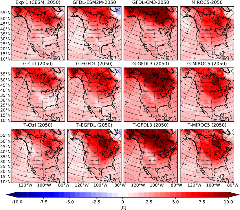
Figure 10. Mean winter season 2 m air temperature anomaly for the 2050–2060 period with respect to the historical period over the outer WRF domain for the GCMs (top row), WRF ensemble members with G physics (middle row), and WRF ensemble members with T physics (bottom row). From left to right are experiments (GCM or GCM driven WRF) associated with CESM1, GFDL-ESM2M, GFDL-CM3, and MIROC5, respectively.
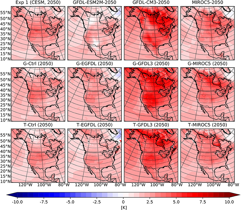
Figure 11. Same as Figure 10 but for the summer season temperature anomalies.
Another important potential implication of this closeness concerns the creation of climate projection forecasts for temperature using bias correction techniques: for the WRF settings used in this study, climate change signal for temperature is well captured at the GCM level, and the bias in the climate forecast result would be primarily in the base climate state. Therefore, bias correcting the GCM base climate state would be sufficient in providing reasonable climate predictions for future periods, at least for similar WRF settings. Other studies have employed bias correction as part of their scheme to forecast future climate (Byun and Hamlet, 2018; Zobel et al., 2018b) and it would be interesting to study future climate projection signals for the CMIP5 ensemble after bias correction. However, this is beyond the scope of this study and left for future works.
Justifying the reliability of GCM predictions in surface temperature warming does not undermine the scientific values of dynamical downscaling experiments, as dynamical downscaling remains capable of improving other variable fields. Precipitation, for example, is strongly dependent on resolution and local processes, and having increased resolution in the climate model will almost certainly improve the quality of precipitation results (Notaro et al., 2013; d'Orgeville et al., 2014; Zobel et al., 2018a). The mid-twenty-first century projection of precipitation changes for the CMIP5 ensemble is showed in Figure 12, where along with similarity between GCM and RCM results, a noticeable difference between results using G or T physics is observed. This means cumulus and microphysics scheme still have their role in refining local precipitation projections. The dependence on physics parametrizations is probably stronger if the outlier physics set ‘g’ described in Peltier et al. (2018) with Morricon microphysics scheme (Morrison et al., 2009), Grell-3 cumulus scheme (Grell and Dévényi, 2002) and Noah MP land surface scheme (Niu et al., 2011) is employed in this study. Details of the physics set dependence on precipitation distributions and precipitation extremes in WRF results over the regional domain of this study are discussed in details in d'Orgeville et al. (2014) and Peltier et al. (2018), so it will not be repeated in this study.
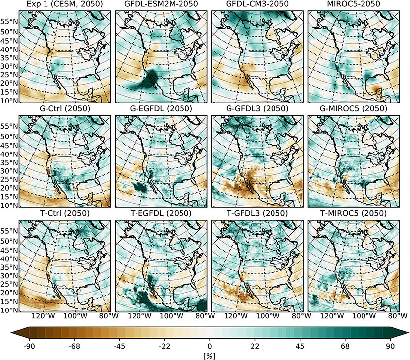
Figure 12. Mean summer season relative change in precipitation for the 2050–2060 period with respect to the historical period over the outer WRF domain for the GCMs (top row), WRF ensemble members with G physics (middle row), and WRF ensemble members with T physics (bottom row). From left to right are experiments (GCM or GCM driven WRF) associated with CESM1, GFDL-ESM2M, GFDL-CM3 and MIROC5 respectively.
Overall, the results of CMIP5 ensemble over future projection periods may be summarized as follows: despite the large difference between WRF and GCM data in the historical period, the climate change signal in surface temperature for the WRF results is closely following the signal in their respective GCM forcing data when comparing to their counterparts in the historical period. Switching between G and T physics parameterizations does not change this closeness in temperature but does affect local change in precipitation projections. These future projection period climate data, along with historical data presented in 3.1, will serve as a reliable database for the extreme heat analysis below.
3.3. Extreme Heat Event Analysis Over the Great Lakes Region Based on the CMIP5 Ensemble Data
On the basis of results from section 3.1, summer season surface temperature between group members differs in magnitude of bias but not in spatial pattern. Therefore, most of our analysis on extreme heat will use a representative ensemble member and we will call upon the full ensemble for only selected analysis. We repeat here for the reader that the definition of a heat wave in this study is “a period with more than three consecutive days of maximum temperatures at or above 32°C/90°F” (section 2.5). Daily data from WRF are used to compute days that have heat wave with temperature and HI metrics and with the same static threshold for all time periods. The wide range of climate covered by our ensemble enables us to explore the change of extreme events around a variety of climate states, and a range of biases. Therefore, no bias correction is applied to the model results before performing this analysis. A direct consequence of this is the preservation of cold biases in the historical results (Figure 6), and therefore we do not expect our extreme heat analysis to match observational records over the historical period.
For our representative ensemble member, we select the simulation with CESM1 forcing and T physics. The first row in Figure 13 compares the number of extreme heat days (computed with surface temperature data and averaged over years within each time period) over the WRF inner domain, between the historical, mid-twenty-first century and end-twenty-first century periods from left to right. During the historical period, extreme heat events are largely confined to the southernmost part of the domain, but they progressively expand to influence most of the land area as the climate change signal strengthens by the end of the century. The number of extreme heat days per year averaged over the GLB (excluding lake surface) increases from 0.5 days during the historical period to 5.7 days during the mid-twenty-first century period to 13.6 days during the end-twenty-first century period. The entire Great Lakes region is largely free from extreme heat events in the historical period, but the number of extreme heat days increases to ~30 days per year south of the lakes and ~5 days per year north of the lakes by the end of the century. The middle row of the figure shows surface relative humidity averaged over the summer season, and which remains moderately high over the domain with little change between the different time periods. When the contribution of this humidity to extreme heat is included through the HI, the region that experiences extreme heat events increases considerably, as displayed in the bottom row of the figure. HI derived number of extreme heat days per year averaged over the GLB also increases to 4.5 days during historical period, 20.9 days during mid-twenty-first century period, and to 42.3 days in end-twenty-first century period. During the historical period, regions south of the Great Lakes experience ~20 extreme heat days per year while such events remain extremely rare north of the Great Lakes. Toward the end of the century, the number of extreme heat days increases to 60–80 days south of the lakes and ~30 days north of the lakes.
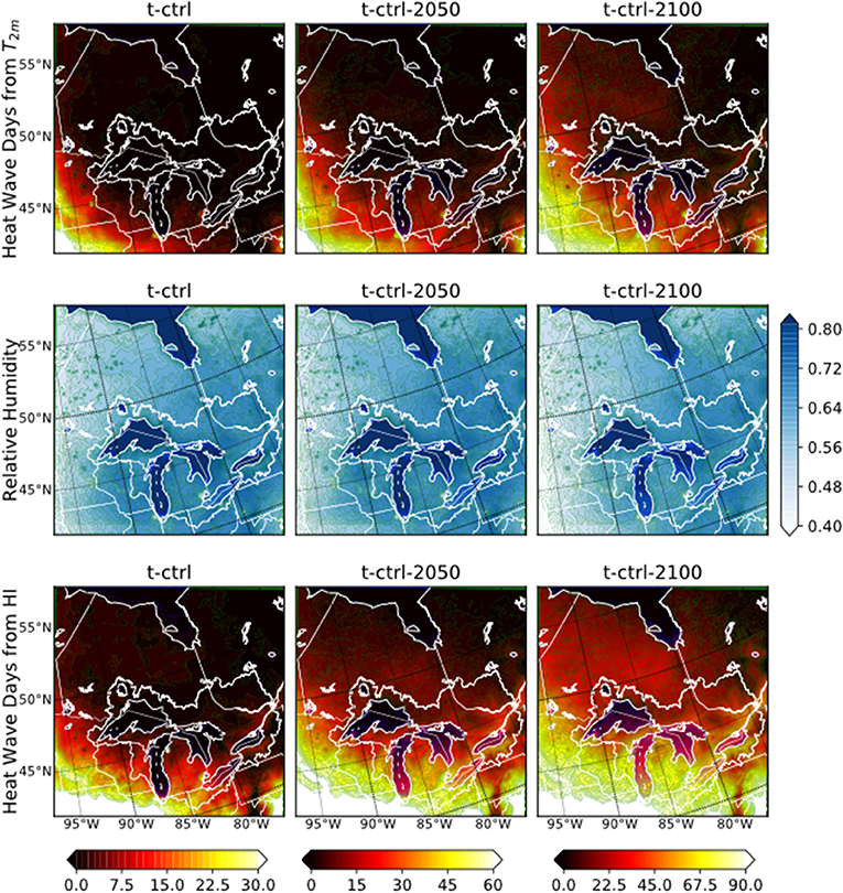
Figure 13. Extreme heat event analysis for simulation with CESM forcing and T physics. The three rows display annually averaged number of extreme heat days per year computed using surface temperature, average summer surface relative humidity, and average number of extreme heat days per year computed using the HI. The three columns represent the historical, mid-twenty-first century and end-twenty-first century time periods. Color bar at the bottom represents the scale used for extreme heat days for each column respectively. Note that the scale of colorbars for heat event days differs between the time periods.
Spatially, it is very clear that the occurrence of extreme heat over the lake surfaces is lower than the surroundings. This is not surprising because the heat capacity of water is much higher than that of the surrounding landscape. Furthermore, when temperature is used as the metric, the number of extreme heat days is significantly lower in regions east of Lake Superior and northeast of Lake Huron compared to other regions at the same latitude. When HI is used the same spatial pattern is obtained, but with reduced magnitude. This is likely due to lake effect: when extremely hot air coming from the south passes over the lakes, both heat conduction and evaporation of lake water extracts sensible heat from that air mass, resulting in cooler air in the downwind region which reduces both temperature and HI. At the same time, the increase in the humidity of the air as it passes over the lakes leads to an increase in the HI. Thus employing the HI accounts for competing influences of lakes, through temperature and moisture, on the likelihood of heat events. The extent of the region with low extreme heat activity is larger than that described by Scott and Huff (1996), and the reasons for this difference will warrant a future study. In our results the differences between the analysis produced using temperature and using the HI is clear and similar for all ensemble members (not shown), and this difference reflects the importance of including moist effects in calculating extreme heat risks in a moist environment.
Influence of lake effects is also visible when the number of extreme heat days over land is zonally averaged, excluding lakes (Figure 14). Regardless of the metric used to determine the occurrence of extreme heat days, the zonally averaged number of heat days decreases as a function of latitude, and which is clearly due to the latitudinal decrease of temperature. However, at the latitudes of Lake Superior (47–49N°), there is a conspicuous drop in the number of days, punctuating the trend of a smooth decrease with latitude. This drop is clearly due to the temperature mitigating effect of the lakes that matches the region with low extreme heat activity described just above. Since part of the mitigation of extreme heat events is associated with the conversion of heat to humidity, the drop is smaller in the HI calculated results that capture moisture effect as part of extreme heat risk. Results over all time periods have this latitudinal drop, while end-twenty-first century result with the clearest signal is presented in Figure 14.
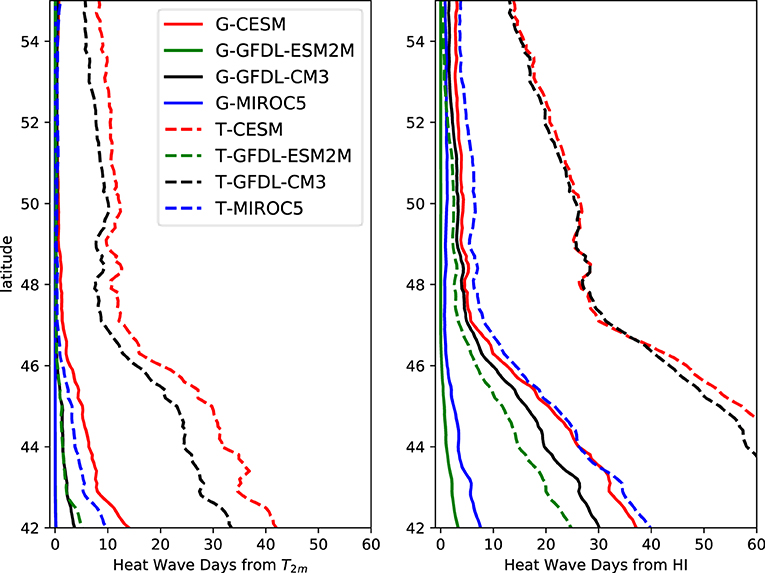
Figure 14. Zonally averaged number of extreme heat days over the central part of the domain (95 − 75W°,41 − 56N°) for all end-century ensemble members. Water surfaces are excluded when taking average.
The dependence of extreme heat activity on the mean climate state is illustrated in Figure 15 where results from all ensemble members is used. Each data point on this figure represents the GLB averaged surface temperature and number of extreme heat days (on a log scale), based upon either temperature or HI, for one ensemble member at one time period. From this figure it is noted first that the number of extreme heat days increase with increasing temperature, which is obvious since the method employed is static. With a rise in temperature, increasing extreme heat events is predicted by almost all studies that discuss extreme event frequency under climate change (see IPCC, 2013b, for a nice summary), regardless of the method of analysis employed. Secondly, when using the temperature metric for extreme, for average temperatures above 18°C (16°C when HI is used), the simulated number of extreme heat days scales roughly linear with respect to average temperature on the log plot, which implies an exponential growth in the number of heat days with temperature. This nonlinear increase of extreme heat days in the coming years deserves attention from policy makers to better understand the associated health risk.
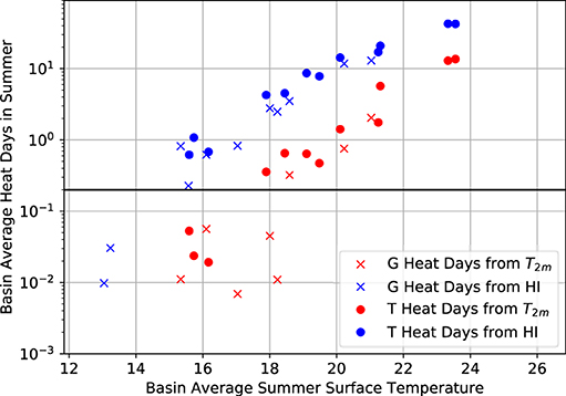
Figure 15. Log plot of annually and spatially averaged number of extreme heat days vs. average summer surface temperature, for all members of the ensemble and all time periods. Dots and crosses represent ensemble members with different physical parameters, red color represent results calculated using temperature, with blue color represents results calculated using the HI. The black line marks reference value of 0.2.
Another point worth noting from Figure 15 is that the exponential dependence of the number of extreme heat days on temperature starts a few degrees earlier using the HI method than temperature. This difference represents the effect of humidity in enhancing the severity of a heat wave event, which is important for a moisture rich region such as the GLB. This signal implies that for regions that have an abundant supply of moisture, increase in extreme heat events will commence earlier than predicted using only temperature as a metric. Future studies focusing on related fields should invest some attention on this moisture effect, to ensure the full risk of extreme heat event is captured.
4. Summary and Discussion
An ensemble of WRF-based dynamically downscaled experiments for climate change projections over the Great Lakes Basin (GLB) has been completed using forcing data from four GCMs. Previous studies using the same dynamical downscaling process (d'Orgeville et al., 2014; Peltier et al., 2018) were focused on validating the experiment setup and model reliability and therefore their physics ensemble was driven only by simulations performed with the CESM1 global model. Here, we use multiple data from several GCMs available in the CMIP5 archive, along with data from our own simulations with CESM1 as forcing for the regional model in order to cover a wide range of possible climate states and to validate the quality of CMIP5 forced WRF results. We also perform analysis of extreme heat events with this ensemble to explore the evolution of such events around the GLB under increasing GHG toward the end of the twenty-first century.
The bias in our ensemble is governed by GCM forcing, WRF physics scheme selection, and inclusion of the lake model. Temperature bias is dominated by large scale effects in the winter season while in summer all sources of biases have first order impact. Precipitation bias in our ensemble is mostly influenced by the cumulus and microphysics schemes used in WRF, and the FLake lake model resolves lake effects effectively around the Great Lakes. However, sources of bias in WRF are not limited to just these factors, as Zobel et al. (2018b) have shown that spectral nudging is capable of generating large differences in WRF results, and Zagar et al. (2013) have shown that there can be uncertainty in WRF results associated with domain size and nesting. Despite large difference between GCM and RCM results in the historical period, the magnitude of climate warming signal is found to be the same between the downscaled simulations and their associated GCMs. This similarity is independent from the physics parametrization employed, indicating that this signal is primarily determined by the large scale circulation features resolved in GCMs, and well captured over the RCM domain by the dynamical downscaling process. Meanwhile, projected changes in local precipitation are still influenced by the physics parametrizations employed, which agrees with findings in previous studies (d'Orgeville et al., 2014; Peltier et al., 2018).
The wide spread of possible climate states in this expanded ensemble provides an excellent basis on which to perform extreme heat event analysis. This analysis reveals a steady increase of extreme heat days with respect to increasing GHG forcing toward the end of the twenty-first century. This increase of extreme heat days with temperature during the projection periods is not surprising, as it would emerge naturally from the definition of extreme heat events used in this study. Meanwhile, our analysis shows that the rate of growth of extreme heat days as a function of surface temperature is independent of physics parametrization and GCM forcing, suggesting that our conclusions for the increase in heat waves toward the end of the century is robust. The extreme heat analysis takes further advantage of the fact that WRF is coupled to a proper lake model (FLake) which helps us simulate the impact of lake effect on the frequency of heat waves in the surrounding regions. A key outcome is the reduction in the number of extreme heat days in the downwind region of the lakes as the lakes absorb heat from the atmosphere.
Along with high temperature, high moisture content in the atmosphere also increases the severity of extreme heat events. The Great Lakes region includes a significant source of moisture, the effect of which on the occurrence of extreme heat events is captured with the HI method for detecting the occurrence of such events. With this method it is shown that the presence of moisture will trigger the onset of extreme heat events in the GLB region at a lower temperature threshold, and that the effect of lake induced sensible cooling in regions downwind of the lakes is also reduced as a result of the conversion of sensible heat to humidity. Since humans are vulnerable to both high temperature and high humidity environments, decision makers should be fully aware of the consequence of high moisture in the Great Lakes region, especially when evaporation from lake surfaces converts high temperature to high relative humidity, leaving a change in the net heat effect that is smaller than that which would be expected from the reduction of air temperature.
Data Availability Statement
The raw data supporting the conclusions of this article will be made available by the authors, without undue reservation.
Author Contributions
FX, AE, and WP contributed to the conception and design of this study. FX, AE, and DC contributed to the software, data analysis and visualization of this study. All authors contributed to discussing the result and preparing the submitted version of the article.
Funding
Support for FX has been provided by NSERC Discovery Grant A9627 to WP.
Conflict of Interest
AE is employed by Aquanty Inc.
The remaining authors declare that the research was conducted in the absence of any commercial or financial relationships that could be construed as a potential conflict of interest.
Publisher's Note
All claims expressed in this article are solely those of the authors and do not necessarily represent those of their affiliated organizations, or those of the publisher, the editors and the reviewers. Any product that may be evaluated in this article, or claim that may be made by its manufacturer, is not guaranteed or endorsed by the publisher.
Acknowledgments
The simulations presented in this manuscript were performed on the SciNet High Performance Computing facility at the University of Toronto, which is a component of the Compute Canada HPC platform. The authors would like to thank Frédéric Laliberté for providing support with using the cdb_query software that processes CMIP5 data.
References
Anderson, G. B., Bell, M. L., and Peng, R. D. (2013). Methods to calculate the heat index as an exposure metric in environmental health research. Environ. Health Perspect. 121, 1111–1119. doi: 10.1289/ehp.1206273
Bates, G. T., Giorgi, F., and Hostetler, S. W. (1993). Toward the simulation of the effects of the great lakes on regional climate. Mon. Weather Rev. 121, 1373–1387. doi: 10.1175/1520-0493(1993)121<1373:TTSOTE>2.0.CO;2
Briley, L. J., Rood, R. B., and Notaro, M. (2021). Large lakes in climate models: a great lakes case study on the usability of cmip5. J. Great Lakes Res. 47, 405–418. doi: 10.1016/j.jglr.2021.01.010
Byun, K., and Hamlet, A. F. (2018). Projected changes in future climate over the midwest and great lakes region using downscaled cmip5 ensembles. Int. J. Climatol. 38, e531–e553. doi: 10.1002/joc.5388
Chen, F., and Dudhia, J. (2001). Coupling an advanced land surface-hydrology model with the penn state-ncar mm5 modeling system. part i: Model implementation and sensitivity. Mon. Weather Rev. 129, 569–585. doi: 10.1175/1520-0493(2001)129<0569:CAALSH>2.0.CO;2
Cheng, G. H., Huang, G. H., Dong, C., Zhu, J. X., Zhou, X., and Yao, Y. (2017). An evaluation of cmip5 gcm simulations over the athabasca river basin, canada. River Res. Appl. 33, 823–843. doi: 10.1002/rra.3136
Collins, W. D., Bitz, C. M., Blackmon, M. L., Bonan, G. B., Bretherton, C. S., Carton, J. A., et al. (2006). The community climate system model version 3 (ccsm3). J. Clim. 19, 2122–2143. doi: 10.1175/JCLI3761.1
Danabasoglu, G., Bates, S. C., Briegleb, B. P., Jayne, S. R., Jochum, M., Large, W. G., et al. (2012). The ccsm4 ocean component. J. Clim. 25, 1361–1389. doi: 10.1175/JCLI-D-11-00091.1
Dee, D. P., Uppala, S. M., Simmons, A. J., Berrisford, P., Poli, P., Kobayashi, S., et al. (2011). The era-interim reanalysis: configuration and performance of the data assimilation system. Q. J. R. Meteorol. Soc. 137, 553–597. doi: 10.1002/qj.828
Deser, C., Phillips, A., Bourdette, V., and Teng, H. (2012). Uncertainty in climate change projections: the role of internal variability. Climate Dyn. 38, 527–546. doi: 10.1007/s00382-010-0977-x
Deser, C., Phillips, A. S., Alexander, M. A., and Smoliak, B. V. (2014). Projecting north american climate over the next 50 years: uncertainty due to internal variability. J. Clim. 27, 2271–2296. doi: 10.1175/JCLI-D-13-00451.1
Donner, L. J., Wyman, B. L., Hemler, R. S., Horowitz, L. W., Ming, Y., Zhao, M., et al. (2011). The dynamical core, physical parameterizations, and basic simulation characteristics of the atmospheric component am3 of the gfdl global coupled model cm3. J. Clim. 24, 3484–3519. doi: 10.1175/2011JCLI3955.1
d'Orgeville, M., Peltier, W. R., Erler, A. R., and Gula, J. (2014). Climate change impacts on great lakes basin precipitation extremes. J. Geophys. Res. Atmos. 119, 10799–10812 doi: 10.1002/2014JD021855
Dunne, J. P., John, J. G., Adcroft, A. J., Griffies, S. M., Hallberg, R. W., Shevliakova, E., et al. (2012). Gfdl's esm2 global coupled climate-carbon earth system models. part i: physical formulation and baseline simulation characteristics. J. Clim. 25, 6646–6665. doi: 10.1175/JCLI-D-11-00560.1
Dunne, J. P., John, J. G., Shevliakova, E., Stouffer, R. J., Krasting, J. P., Malyshev, S. L., et al. (2013). GFDL's ESM2 global coupled climate?carbon earth system models. part ii: carbon system formulation and baseline simulation characteristics. J. Clim. 26, 2247–2267. doi: 10.1175/JCLI-D-12-00150.1
Erler, A. R. (2015). High Resolution Hydro-climatological Projections for Western Canada (Ph.D. thesis). University of Toronto.
Erler, A. R., and Peltier, W. R. (2016). Projected changes in precipitation extremes for western canada based on high-resolution regional climate simulations. J. Clim. 29, 8841–8863. doi: 10.1175/JCLI-D-15-0530.1
Erler, A. R., and Peltier, W. R. (2017). Projected hydroclimatic changes in two major river basins at the canadian west coast based on high-resolution regional climate simulations. J. Clim. 30, 8081–8105. doi: 10.1175/JCLI-D-16-0870.1
Erler, A. R., Peltier, W. R., and D'Orgeville, M. (2015). Dynamically downscaled high-resolution hydroclimate projections for western canada. J. Clim. 28, 423–450. doi: 10.1175/JCLI-D-14-00174.1
Fouquart, Y., Buriez, J. C., Herman, M., and Kandel, R. S. (1990). The influence of clouds on radiation: A climate-modeling perspective. Reviews of Geophysics, 28, 145–166. doi: 10.1029/RG028i002p00145
Gent, P. R., Danabasoglu, G., Donner, L. J., Holland, M. M., Hunke, E. C., Jayne, S. R., et al. (2011). The community climate system model version 4. J. Clim. 24, 4973–4991. doi: 10.1175/2011JCLI4083.1
Grell, G. A., and Dévényi, D. (2002). A generalized approach to parameterizing convection combining ensemble and data assimilation techniques. Geophys. Res. Lett. 29, 38-1–38-4. doi: 10.1029/2002GL015311
Griffies, S. M., Winton, M., Donner, L. J., Horowitz, L. W., Downes, S. M., Farneti, R., et al. (2011). The gfdl cm3 coupled climate model: Characteristics of the ocean and sea ice simulations. J. Clim. 24, 3520–3544. doi: 10.1175/2011JCLI3964.1
Gula, J., and Peltier, W. R. (2012). Dynamical downscaling over the great lakes basin of north america using the wrf regional climate model: the impact of the great lakes system on regional greenhouse warming. J. Clim. 25, 7723–7742. doi: 10.1175/JCLI-D-11-00388.1
Holland, M. M., Bailey, D. A., Briegleb, B. P., Light, B., and Hunke, E. (2012). Improved sea ice shortwave radiation physics in ccsm4: The impact of melt ponds and aerosols on arctic sea ice. J. Clim. 25, 1413–1430. doi: 10.1175/JCLI-D-11-00078.1
Hong, S.-Y., and Lim, J.-O. J. (2006). The WRF single-moment 6-class microphysics scheme (WSM6). J. Korean Meteor. Soc, 42, 129–151.
Huo, Y., and Peltier, W. R. (2019). Dynamically downscaled climate simulations of the indian monsoon in the instrumental era: physics parameterization impacts and precipitation extremes. J. Appl. Meteorol. Climatol. 58, 831–852. doi: 10.1175/JAMC-D-18-0226.1
Huo, Y., Peltier, W. R., and Chandan, D. (2021). Mid-holocene monsoons in south and southeast asia: dynamically downscaled simulations and the influence of the green sahara. Clim. Past 17, 1645–1664. doi: 10.5194/cp-17-1645-2021
Iacono, M. J., Delamere, J. S., Mlawer, E. J., Shephard, M. W., Clough, S. A., and Collins, W. D. (2008). Radiative forcing by long-lived greenhouse gases: calculations with the aer radiative transfer models. J. Geophys. Res. Atmos. 113:D13103. doi: 10.1029/2008JD009944
IPCC (2013a). The Fifth Assessment Report (AR5) of the United Nations Intergovernmental Panel on Climate Change (IPCC), Climate Change 2013: The Physical Science Basis, IPCC WGI AR5, Chapter 14. Cambridge; New York, NY: Cambridge University Press; Climate Phenomena and their Relevance for Future Regional Climate Change.
IPCC (2013b). The Fifth Assessment Report (AR5) of the United Nations Intergovernmental Panel on Climate Change (IPCC), Climate Change 2013: The Physical Science Basis, IPCC WGI AR5, Chapter 9. Cambridge University Press; Evaluation of Climate Models.
Jeong, D. I., Sushama, L., Diro, G. T., Khaliq, M. N., Beltrami, H., and Caya, D. (2016). Projected changes to high temperature events for canada based on a regional climate model ensemble. Clim. Dyn. 46, 3163–3180. doi: 10.1007/s00382-015-2759-y
Kain, J. S. (2004). The kain?fritsch convective parameterization: An update. J. Appl. Meteorol. 43, 170–181. doi: 10.1175/1520-0450(2004)043<0170:TKCPAU>2.0.CO;2
Kharin, V. V., Zwiers, F. W., Zhang, X., and Wehner, M. (2013). Changes in temperature and precipitation extremes in the cmip5 ensemble. Clim. Change 119, 345–357. doi: 10.1007/s10584-013-0705-8
Kug, J.-S., Jeong, J.-H., Jang, Y.-S., Kim, B.-M., Folland, C. K., Min, S.-K., et al. (2015). Two distinct influences of arctic warming on cold winters over north america and east asia. Nat. Geosci. 8, 759–762. doi: 10.1038/ngeo2517
Kumar, S., Kinter, J., Dirmeyer, P. A., Pan, Z., and Adams, J. (2013). Multidecadal climate variability and the “warming hole” in north america: results from cmip5 twentieth- and twenty-first-century climate simulations. J. Clim. 26, 3511–3527. doi: 10.1175/JCLI-D-12-00535.1
Lawrence, D. M., Oleson, K. W., Flanner, M. G., Fletcher, C. G., Lawrence, P. J., Levis, S., et al. (2012). The ccsm4 land simulation, 1850–2005: assessment of surface climate and new capabilities. J. Clim. 25, 2240–2260. doi: 10.1175/JCLI-D-11-00103.1
Li, C., Zhang, X., Zwiers, F., Fang, Y., and Michalak, A. M. (2017). Recent very hot summers in northern hemispheric land areas measured by wet bulb globe temperature will be the norm within 20 years. Earths Future 5, 1203–1216. doi: 10.1002/2017EF000639
Li, K., Zhang, J., and Wu, L. (2018). Assessment of soil moisture-temperature feedbacks with the ccsm-wrf model system over east asia. J. Geophys. Res. Atmos. 123, 6822–6839. doi: 10.1029/2017JD028202
Lofgren, B. M. (1997). Simulated effects of idealized laurentian great lakes onregional and large-scale climate. J. Clim. 10, 2847–2858. doi: 10.1175/1520-0442(1997)010<2847:SEOILG>2.0.CO;2
Mallard, M. S., Nolte, C. G., Bullock, O. R., Spero, T. L., and Gula, J. (2014). Using a coupled lake model with wrf for dynamical downscaling. J. Geophys. Res. Atmos. 119, 7193–7208. doi: 10.1002/2014JD021785
Maloney, E. D., Camargo, S. J., Chang, E., Colle, B., Fu, R., Geil, K. L., et al. (2014). North american climate in cmip5 experiments: Part iii: assessment of twenty-first-century projections. J. Clim. 27, 2230–2270. doi: 10.1175/JCLI-D-13-00273.1
McKenney, D. W., Hutchinson, M. F., Papadopol, P., Lawrence, K., Pedlar, J., Campbell, K., et al. (2011). Customized spatial climate models for north america. Bull. Am. Meteorol. Soc. 92, 1611–1622. doi: 10.1175/2011BAMS3132.1
Meehl, G. A., and Tebaldi, C. (2004). More intense, more frequent, and longer lasting heat waves in the 21st century. Science 305, 994–997. doi: 10.1126/science.1098704
Mironov, D. V. (2008). Parameterization of lakes in numerical weather prediction. description of a lake model. Technical report, Deutscher Wetterdienst, Offenbach am Main, Germany.
Morrison, H., Thompson, G., and Tatarskii, V. (2009). Impact of cloud microphysics on the development of trailing stratiform precipitation in a simulated squall line: comparison of one- and two-moment schemes. Mon. Weather Rev. 137, 991–1007. doi: 10.1175/2008MWR2556.1
Nakanishi, M., and Niino, H. (2009). Development of an improved turbulence closure model for the atmospheric boundary layer. J. Meteor. Soc. Jpn 87, 895–912. doi: 10.2151/jmsj.87.895
Neale, R. B., Richter, J., Park, S., Lauritzen, P. H., Vavrus, S. J., Rasch, P. J., et al. (2013). The mean climate of the community atmosphere model (cam4) in forced sst and fully coupled experiments. J. Clim. 26, 5150–5168. doi: 10.1175/JCLI-D-12-00236.1
Niu, G.-Y., Yang, Z.-L., Mitchell, K. E., Chen, F., Ek, M. B., Barlage, M., et al. (2011). The community noah land surface model with multiparameterization options (noah-mp): 1. model description and evaluation with local-scale measurements. J. Geophys. Res. Atmos. 116:D12. doi: 10.1029/2010JD015139
Notaro, M., Bennington, V., and Lofgren, B. (2015a). Dynamical downscaling?based projections of great lakes water levels. J. Clim. 28, 9721–9745. doi: 10.1175/JCLI-D-14-00847.1
Notaro, M., Bennington, V., and Vavrus, S. (2015b). Dynamically downscaled projections of lake-effect snow in the great lakes basin. J. Clim. 28, 1661–1684. doi: 10.1175/JCLI-D-14-00467.1
Notaro, M., Holman, K., Zarrin, A., Fluck, E., Vavrus, S., and Bennington, V. (2013). Influence of the laurentian great lakes on regional climate. J. Clim. 26, 789–804. doi: 10.1175/JCLI-D-12-00140.1
Notaro, M., Zhong, Y., Xue, P., Peters-Lidard, C., Cruz, C., Kemp, E., et al. (2021). Cold season performance of the nu-wrf regional climate model in the great lakes region. J. Hydrometeorol. 22, 2423–2454. doi: 10.1175/JHM-D-21-0025.1
O'Reilly, C. M., Sharma, S., Gray, D. K., Hampton, S. E., Read, J. S., Rowley, R. J., et al. (2015). Rapid and highly variable warming of lake surface waters around the globe. Geophys. Res. Lett. 42, 10773–10781. doi: 10.1002/2015GL066235
Paynter, D., Frölicher, T. L., Horowitz, L. W., and Silvers, L. G. (2018). Equilibrium climate sensitivity obtained from multimillennial runs of two gfdl climate models. J. Geophys. Res. Atmos. 123, 1921–1941. doi: 10.1002/2017JD027885
Peings, Y., Cattiaux, J., Vavrus, S., and Magnusdottir, G. (2017). Late twenty-first-century changes in the midlatitude atmospheric circulation in the cesm large ensemble. J. Clim. 30, 5943–5960. doi: 10.1175/JCLI-D-16-0340.1
Peltier, W. R., d'Orgeville, M., Erler, A. R., and Xie, F. (2018). Uncertainty in future summer precipitation in the laurentian great lakes basin: dynamical downscaling and the influence of continental-scale processes on regional climate change. J. Clim. 31, 2651–2673. doi: 10.1175/JCLI-D-17-0416.1
Perkins, S. E., and Alexander, L. V. (2013). On the measurement of heat waves. J. Clim. 26, 4500–4517. doi: 10.1175/JCLI-D-12-00383.1
Peterson, T. C., Zhang, X., Brunet-India, M., and Vázquez-Aguirre, J. L. (2008). Changes in north american extremes derived from daily weather data. J. Geophys. Res. Atmos. 113:D7. doi: 10.1029/2007JD009453
Philip, S. Y., Kew, S. F., van Oldenborgh, G. J., Yang, W., Vecchi, G. A., Anslow, F. S., et al. (2021). Rapid attribution analysis of the extraordinary heatwave on the pacific coast of the us and canada june 2021. Technical report.
Robinson, P. J. (2001). On the definition of a heat wave. J. Appl. Meteorol. 40, 762–775. doi: 10.1175/1520-0450(2001)040<0762:OTDOAH>2.0.CO;2
Saha, S., Moorthi, S., Pan, H.-L., Wu, X., Wang, J., Nadiga, S., et al. (2010). The ncep climate forecast system reanalysis. Bull. Am. Meteorol. Soc. 91, 1015–1058. doi: 10.1175/2010BAMS3001.1
Scott, R. W., and Huff, F. A. (1996). Impacts of the great lakes on regional climate conditions. J. Great Lakes Res. 22, 845–863. doi: 10.1016/S0380-1330(96)71006-7
Sheffield, J., Barrett, A. P., Colle, B., Fernando, D. N., Fu, R., Geil, K. L., et al. (2013a). North american climate in cmip5 experiments. part i: evaluation of historical simulations of continental and regional climatology*. J. Clim. 26, 9209–9245. doi: 10.1175/JCLI-D-12-00592.1
Sheffield, J., Camargo, S. J., Fu, R., Hu, Q., Jiang, X., Johnson, N., et al. (2013b). North american climate in cmip5 experiments. part ii: evaluation of historical simulations of intraseasonal to decadal variability. J. Clim. 26, 9247–9290. doi: 10.1175/JCLI-D-12-00593.1
Sillmann, J., Kharin, V. V., Zhang, X., Zwiers, F. W., and Bronaugh, D. (2013a). Climate extremes indices in the cmip5 multimodel ensemble: Part 1. model evaluation in the present climate. J. Geophys. Res. Atmos. 118, 1716–1733. doi: 10.1002/jgrd.50203
Sillmann, J., Kharin, V. V., Zwiers, F. W., Zhang, X., and Bronaugh, D. (2013b). Climate extremes indices in the cmip5 multimodel ensemble: Part 2. future climate projections. J. Geophys. Res. Atmos. 118, 2473–2493. doi: 10.1002/jgrd.50188
Skamarock, W. C., and Klemp, J. B. (2008). A time-split nonhydrostatic atmospheric model for weather research and forecasting applications. J. Comput. Phys. 227, 3465–3485. doi: 10.1016/j.jcp.2007.01.037
Song, Y., and Yu, Y. (2015). Impacts of external forcing on the decadal climate variability in cmip5 simulations. J. Clim. 28, 5389–5405. doi: 10.1175/JCLI-D-14-00492.1
Taylor, K. E., Stouffer, R. J., and Meehl, G. A. (2012). An overview of cmip5 and the experiment design. Bull. Am. Meteorol. Soc. 93, 485–498. doi: 10.1175/BAMS-D-11-00094.1
Thompson, G., Tewari, M., Ikeda, K., Tessendorf, S., Weeks, C., Otkin, J., et al. (2016). Explicitly-coupled cloud physics and radiation parameterizations and subsequent evaluation in wrf high-resolution convective forecasts. Atmospheric Research, 168, 92–104. doi: 10.1016/j.atmosres.2015.09.005
Vautard, R., van Aalst, M., Boucher, O., Drouin, A., Haustein, K., Kreienkamp, F., et al. (2020). Human contribution to the record-breaking june and july 2019 heatwaves in western europe. Environ. Res. Lett. 15:094077. doi: 10.1088/1748-9326/aba3d4
Watanabe, M., Suzuki, T., O'ishi, R., Komuro, Y., Watanabe, S., Emori, S., et al. (2010). Improved climate simulation by miroc5: mean states, variability, and climate sensitivity. J. Clim. 23, 6312–6335. doi: 10.1175/2010JCLI3679.1
Woolway, R. I., Kraemer, B. M., Lenters, J. D., Merchant, C. J., O'Reilly, C. M., and Sharma, S. (2020). Global lake responses to climate change. Nat. Rev. Earth Environ. 1, 388–403. doi: 10.1038/s43017-020-0067-5
Xue, P., Pal, J. S., Ye, X., Lenters, J. D., Huang, C., and Chu, P. Y. (2017). Improving the simulation of large lakes in regional climate modeling: two-way lake?atmosphere coupling with a 3d hydrodynamic model of the great lakes. J. Clim. 30, 1605–1627. doi: 10.1175/JCLI-D-16-0225.1
Zagar, N., Honzak, L., Zabkar, R., Skok, G., Rakovec, J., and Ceglar, A. (2013). Uncertainties in a regional climate model in the midlatitudes due to the nesting technique and the domain size. J. Geophys. Res. Atmos. 118, 6189–6199. doi: 10.1002/jgrd.50525
Zobel, Z., Wang, J., Wuebbles, D. J., and Kotamarthi, V. R. (2018a). Analyses for high-resolution projections through the end of the 21st century for precipitation extremes over the united states. Earths Future 6, 1471–1490. doi: 10.1029/2018EF000956
Zobel, Z., Wang, J., Wuebbles, D. J., and Kotamarthi, V. R. (2018b). Evaluations of high-resolution dynamically downscaled ensembles over the contiguous united states. Clim. Dyn. 50, 863–884. doi: 10.1007/s00382-017-3645-6
A1. Heat Index Equation
Heat Index (HI) equation we use following https://www.wpc.ncep.noaa.gov/html/heatindex_equation.shtml is given as:
where T is temperature in degrees Fahrenheit and RH is relative humidity in percent. HI is the heat index expressed as an apparent temperature in degrees Fahrenheit. If the RH is less than 13% and the temperature is between 80°F and 112°F, then the following adjustment is subtracted from HI:
On the other hand, if the RH is greater than 85% and the temperature is between 80°F and 87°F, then the following adjustment is added to HI:
An alternative equation is used when heat index value is expected to fall below about 80°F where the regression analysis that leads to the main HI equation becomes inappropriate. The alternative simpler equation is the following:
However, this alternative equation is less relevant for this study since HI threshold for extreme heat events is 32°C=89.6°F that is strictly above the 80°F limit.
Keywords: FLake, CMIP5, WRF, climate change, extreme heat event, Great Lakes (North America)
Citation: Xie F, Erler AR, Chandan D and Peltier WR (2021) Great Lakes Basin Heat Waves: An Analysis of Their Increasing Probability of Occurrence Under Global Warming. Front. Water 3:782265. doi: 10.3389/frwa.2021.782265
Received: 24 September 2021; Accepted: 01 November 2021;
Published: 13 December 2021.
Edited by:
Julie A. Winkler, Michigan State University, United StatesReviewed by:
Jimy Dudhia, National Center for Atmospheric Research (UCAR), United StatesJoni-Pekka Pietikäinen, Climate Service Center Germany (GERICS), Germany
Copyright © 2021 Xie, Erler, Chandan and Peltier. This is an open-access article distributed under the terms of the Creative Commons Attribution License (CC BY). The use, distribution or reproduction in other forums is permitted, provided the original author(s) and the copyright owner(s) are credited and that the original publication in this journal is cited, in accordance with accepted academic practice. No use, distribution or reproduction is permitted which does not comply with these terms.
*Correspondence: Fengyi Xie, ZmVuZ3lpLnhpZUBtYWlsLnV0b3JvbnRvLmNh; W. Richard Peltier, cGVsdGllckBhdG1vc3AucGh5c2ljcy51dG9yb250by5jYQ==