 Victoria M. H. Deman1
 Akash Koppa1
 Willem Waegeman2David A. MacLeod3Michael Bliss Singer4,5,6
 Diego G. Miralles1*
- 1Hydro-Climate Extremes Laboratory, Ghent University, Ghent, Belgium
- 2Department of Data Analysis and Mathematical Modelling, Ghent University, Ghent, Belgium
- 3School of Geographical Sciences, University of Bristol, Bristol, United Kingdom
- 4School of Earth and Environmental Sciences, Cardiff University, Cardiff, United Kingdom
- 5Water Research Institute, Cardiff University, Cardiff, United Kingdom
- 6Earth Research Institute, University of California, Santa Barbara, Santa Barbara, CA, United States
The Horn of Africa is highly vulnerable to droughts and floods, and reliable long-term forecasting is a key part of building resilience. However, the prediction of the “long rains” season (March–May) is particularly challenging for dynamical climate prediction models. Meanwhile, the potential for machine learning to improve seasonal precipitation forecasts in the region has yet to be uncovered. Here, we implement and evaluate four data-driven models for prediction of long rains rainfall: ridge and lasso linear regressions, random forests and a single-layer neural network. Predictors are based on SSTs, zonal winds, land state, and climate indices, and the target variables are precipitation totals for each separate month (March, April, and May) in the Horn of Africa drylands, with separate predictions made for lead-times of 1–3 months. Results reveal a tendency for overfitting when predictors are preselected based on correlations to the target variable over the entire historical period, a frequent practice in machine learning-based seasonal forecasting. Using this conventional approach, the data-driven methods—and particularly the lasso and ridge regressions—often outperform dynamical seasonal hindcasts. However, when the selection of predictors is done independently of both the train and test data, by performing this predictor selection within the cross-validation loop, the performance of all four data-driven models is poorer than that of the dynamical hindcasts. These findings should not discourage future applications of machine learning for rainfall forecasting in the region. Yet, they should be seen as a note of caution to prevent optimistically biased results that are not indicative of the true power in operational forecast systems.
1. Introduction
Accurate seasonal forecasts could bring enormous societal benefits and lead to improved agricultural productivity, water resource management, and disaster response planning (He et al., 2021). There is a growing interest from governments, industries, and non-governmental organizations (NGOs) in seasonal forecasts that could support early actions to weather extremes (Lang et al., 2020; Merryfield et al., 2020). As a consequence, seasonal timescales, lying between the short range weather forecasts and long range climate projections, have been receiving increasing attention by the forecast community (Bauer et al., 2015; Merryfield et al., 2020). However, traditional weather forecast models were not originally designed for those timescales (Cohen et al., 2019). Skilful seasonal predictions require accurate characterization of “slowly-changing” climate variables that influence weather conditions over weeks to months. These include ocean temperatures, persistent atmospheric pressure patterns, land conditions, and sea ice (Mariotti et al., 2020). Despite the progress in the representation of these variables in weather models (Merryfield et al., 2020), error propagation still limits predictive power at seasonal scales (Cohen et al., 2019). These factors suggest a need for a different approach that can leverage the plethora of reanalysis data and observations from satellite remote sensing.
Artificial Intelligence (AI) has the potential to revolutionize multiple research fields, and the arena of weather and climate prediction is no exception (Reichstein et al., 2019; Zhao et al., 2019). While the limited volumes of high-quality climate observations, along with their strong spatiotemporal correlation and high-dimensionality, impose a great challenge for AI algorithms (Cohen et al., 2019), pure AI forecasting models may already exhibit skills that are comparable to conventional weather forecast models, even at short time scales (Scher, 2018). A recent review of the use of AI for weather forecast modeling even stated that it is conceivable that numerical weather models may one day become obsolete (Schultz et al., 2021). Yet, as of today, the best practical results can still be expected from a combination of AI and physical models (Cohen et al., 2019; Schultz et al., 2021). If seasonal climate predictions were improved by incorporating AI, this could help support socioeconomic preparedness and resilience, particularly in regions with significant exposure to seasonal climate hazards. Nonetheless, only a limited number of machine learning studies have focused on seasonal prediction so far (Dewitte et al., 2021), and seasonal timescales are often only briefly mentioned in surveys (Nayak et al., 2013). Comprehensive reviews on machine learning in seasonal prediction include Cohen et al. (2019) and Bochenek and Ustrnul (2022). Cohen et al. (2019), in particular, argued that machine learning can be adopted to further improve the accuracy of operational seasonal predictions, a field that almost exclusively relies on complex fully coupled dynamical forecast systems to date.
The Horn of Africa—including the countries of Djibouti, Eritrea, Ethiopia, Kenya, and Somalia—is one of those regions. The rainfall in this region is characterized by two main seasons—long (March–May, MAM) and short (October–December, OND) rains. Not only is it host to a large rural population that is dependent on this highly seasonal rainfall supply, but it is also regularly exposed to climatic extremes such as droughts and floods. Moreover, the prediction via dynamical models is notoriously challenging in the region. Chronic droughts occurred during the periods 2005–2006 and 2008–2011, which faced rainfall deficits of 30–75% below average (Nicholson, 2014a; Funk et al., 2019). The 2011 crisis, partly caused by the drought event, affected millions of people and resulted in significant displacement of communities, with millions suffering from loss of livelihoods and assets (Slim, 2012). Flood conditions arose after the drought that ended in the second half of 2011, aggravating the already critical humanitarian situation in the region (Nicholson, 2014a). These extreme events and difficulties associated with them are still ongoing: in April–May 2020 and August 2021 Ethiopia experienced flash floods affecting more than 100,000 people (Davies, 2021). At the time of this article, four consecutive rain seasons failing, starting from October 2020 have resulted in millions of people in Ethiopia, Somalia and Kenya facing food insecurity and water shortages in the present (UN OCHA, 2022). These below-normal rainfall seasons have not always been anticipated by existing dynamical forecast systems in the region, particularly for the long rain seasons (March–May, MAM). More accurate drought predictions are sorely needed, and AI techniques offer a potential opportunity to overcome limitations in dynamical models (Cohen et al., 2019).
To date, efforts to use data-driven approaches for seasonal prediction in the Horn of Africa remain limited. Mwale and Gan (2005) used artificial neural networks, where the parameters were optimized using genetic algorithms, to predict September–November precipitation with a one-season lead-time over eastern Africa. They achieved forecast skills that overcame those by linear methods (Ntale et al., 2003). More recently, Alhamshry et al. (2019) constructed an Elman recurrent neural network model to forecast summer rainfall from teleconnected SSTs over the Lake Tana Basin in Ethiopia, with good results over the region. However, seasonal forecasts targeting Horn of Africa's long rains using data-driven learning approaches are especially rare or non-existent. Moreover, Alhamshry et al. (2019), as well as multiple other studies using AI for seasonal weather prediction in other regions, used SSTs over preselected regions based on a preassessment of the correlations between SSTs and rainfall over the entire historical period. This approach is prone to overfitting, due to the dependency between predictor variables and test data, and could give optimistically biased results (Hastie et al., 2009).
This study assesses the predictability of the Horn of Africa's rainfall using data-driven approaches. The focus is on the long rains, as it is not only understudied in this context, but also particularly challenging to dynamical weather forecasts and crucial for the supply of water to the region (Camberlin and Philippon, 2002; Nicholson, 2014b). The study specifically focuses on drylands, as they are home to many agropastoral communities with a lifestyle that is highly dependent on water, and thus rainfall, making the region especially susceptible to disasters resulting from climate extremes such as the ongoing drought event. Four different data-driven methods are explored: ridge and lasso linear regression, random forests and single-layer neural networks. The goal is to assess the potential of these methods in forecasting MAM rainfall for lead-times from 1 to 3 months. Predictors of the long rains are based on SSTs, zonal winds, land state and climate indices. A specific focus is placed on investigating the influence of including predictors that are preselected based on correlations to the target variable, a frequent practice in machine learning-based seasonal forecasting.
2. Study area
The focus of this study is the Horn of Africa drylands, encompassing Somalia, northern Kenya and a part of eastern Ethiopia (Figure 1). The study area is selected to highlight the bimodal seasonality of rainfall as per (Adloff et al., 2022), including grid cells for which the climatological rainfall over February, July, and September is below 30 mm. Most of the region is characterized by a flat topography mainly consisting of lowlands, plateaus and coastal plains with an arid and semiarid climate. It borders the Gulf of Aden in the north and the Indian Ocean to the east. To the west and southwest, it is bounded by the Ethiopian highlands and the East African highlands, respectively. The area has a bimodal rainfall regime, with so-called long and a short rainfall season, which are consistently relied upon for regional lives and livelihoods (Figure 1), and a yearly average rainfall amount of ~311 mm. While the interannual variability of the short rains is strongly associated with coupled ocean–atmosphere oscillations, specifically the El Niño Southern Oscillation (ENSO) and the Indian Ocean Dipole (Behera et al., 2005; Manatsa and Behera, 2013; Nicholson, 2015a; MacLeod et al., 2021), the drivers of the long rains are more complex. Vellinga and Milton (2018) suggests that the most significant factors influencing long rains variability are: the Madden-Julian Oscillation (MJO), SST in the north-west Indian Ocean, and the Quasi-Biennial Oscillation. Recent evidence has suggested the association of a fast-warming region in the west Pacific Ocean, termed as “Western V”, with the frequency of droughts during the long rain season, and its long term drying (Funk et al., 2018). As mentioned above, our specific focus is on the long rains, which contribute a total of 134 mm (±43%). The region exhibits a north–south gradient in rainfall, with the northern tip of the Horn receiving very low volumes.
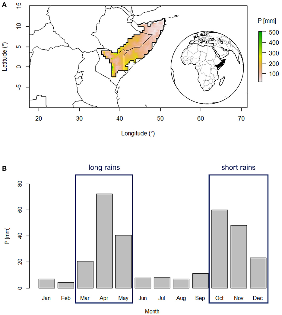
Figure 1. Study area climatology. (A) Location of the study region and average total long rains (MAM) rainfall P (mm). (B) Precipitation data from CenTrends (Funk et al., 2018) based on 1981–2014. The area has been delimited based on Adloff et al. (2022).
3. Data and methods
Four data-driven models are compared in their skill to hindcast the long rains in the Horn of Africa drylands (Section 3.1). Their input data consist of reanalysis and satellite data of multiple atmospheric, land and ocean variables (Section 3.3). Forecast models were developed for every month of the long rains season separately, at lead-times of 1–3 months. Here, a 1-month lead time refers to data used of 1 month before the target month. Nested k-fold cross-validation is used to assess their performance (Section 3.2). March, April, and May are considered separately because the long rains season is not homogeneous, and rainfall is only mildly correlated among the different months (Camberlin and Philippon, 2002; Nicholson, 2014b, 2015b). The time period used in this study is 1981–2014, capped by rainfall and vegetation greenness data availability. Furthermore, two approaches for predictor selection are adopted (Section 3.4): one in which the predictors were selected based on correlations on the whole available dataset (A1) and one where correlation-based predictor selection was performed within the cross-validation loop (A2). Results are compared against the dynamical SEAS5 hindcasts produced at the European Centre for Medium-Range Weather Forecasts (Johnson et al., 2019).
3.1. Prediction models
3.1.1. Ridge regression
Ridge regression is a regularization method designed to deal with covarying predictors, and it reduces overfitting by shrinking model coefficients toward zero. Since data for this study is scarce with a high number of predictors (N < p), shrinkage methods are particularly appropriate (Hastie et al., 2009). The ridge regression is a linear method that employs an iterative shrinking operation, rather than for example focusing on subsets. The regression coefficients in ridge regression are shrunk toward zero and each other by imposing a penalty on their size, thus reducing model capacity. The amount of shrinkage is controlled by a parameter λ≥0; smaller λ values give a smaller amount of shrinkage (Hastie et al., 2009). The ridge coefficients aim to minimize a penalized residual sum of squares (Equation 1).
with the ridge estimate, yi the targets, xi,j the inputs, β0 the intercept, βj the coefficient estimates, λ the penalty factor, p the number of predictors and N the number of observations.
3.1.2. Lasso regression
Similar to the ridge regression, lasso is also a regularization method designed to deal with covarying predictors, and thus it reduces overfitting by shrinking model coefficients toward zero. Lasso stands for “least absolute shrinkage and selection operator”, and it penalizes the absolute value of the model coefficients. In contrast to ridge regression, the lasso regression procedure (Equation 2) can produce coefficients that are exactly zero and thus reduce the number of model parameters. In the case of correlated predictors, lasso might randomly select one predictor over the other (Tibshirani, 1996; Hastie et al., 2009).
with the lasso estimate, and every other variable defined as in Equation (1).
3.1.3. Random forest
Random forests is an ensemble learning technique in which a collection of regression trees is fitted to bootstrapped versions of the training data (Breiman, 2001). Random forests are suitable for a wide range of prediction problems, as they are simple to use with only a few parameters to tune (Hastie et al., 2009; Biau and Scornet, 2016), and have shown good performances in settings with a small sample size and a high-dimensional predictor space (Biau and Scornet, 2016). They are particularly recommended in case of complex non-linear interactions (Hastie et al., 2009). For new instances, the predictions of individual regression trees are averaged to obtain a final prediction (a.k.a. bagging). Bagging reduces variance by averaging many noisy, but approximately unbiased models. The random forest regression predictor after B trees are grown is shown in Equation (3).
with Θb the bth random forest tree in terms of split variables, cutpoints at each node and terminal-node values (Hastie et al., 2009).
3.1.4. Neural network
Neural networks are defined as a network of interconnected nodes where information processing occurs. Connection links pass signals between the nodes, each with an associated weight that represents its connection strength. A non-linear transformation, known as an activation function, is applied to the net input of each node in order to determine the output signal. The most common type of neural networks are multilayer perceptrons, which consist of an input layer, at least one hidden layer and an output layer, where information flows in a single direction only, from the input to the output layer. The number of predictors and target variables determines the number of input and output nodes, respectively. Hidden layers allow for non-linearity in the relationship between the inputs and outputs. The number of hidden layers and neurons depends on the problem and data availability (Mekanik et al., 2013). Here, a multilayer perceptron with a single hidden layer is used: since we have a low number of samples with a high number of predictors, this helps reduce the risk of overfitting.
3.2. Cross-validation
To compare the performance of each model, a nested k-fold cross-validation is used (see Supplementary material for the pseudocode). This procedure is more appropriate than a single split into training and testing data, since the sample size is relatively low (Varma and Simon, 2006; Wainer and Cawley, 2021). Nested cross-validation requires two cross-validation steps, referred to as the outer and inner loops. In the outer loop, datasets are split into k groups, or folds, in which the models, generated in the inner loop, are evaluated by determining unbiased performance estimates. In the outer loop, each fold is once held out for testing, and the remaining k–1 folds are then merged and split into inner folds for training (Wainer and Cawley, 2021). For this study, a five-fold cross validation in the outer loop and a four-fold cross-validation in the inner loop are chosen (Figure 2). These values are decided based on a trade-off between having enough folds with performance estimates, having enough data to calculate a performance metric, and compute time.
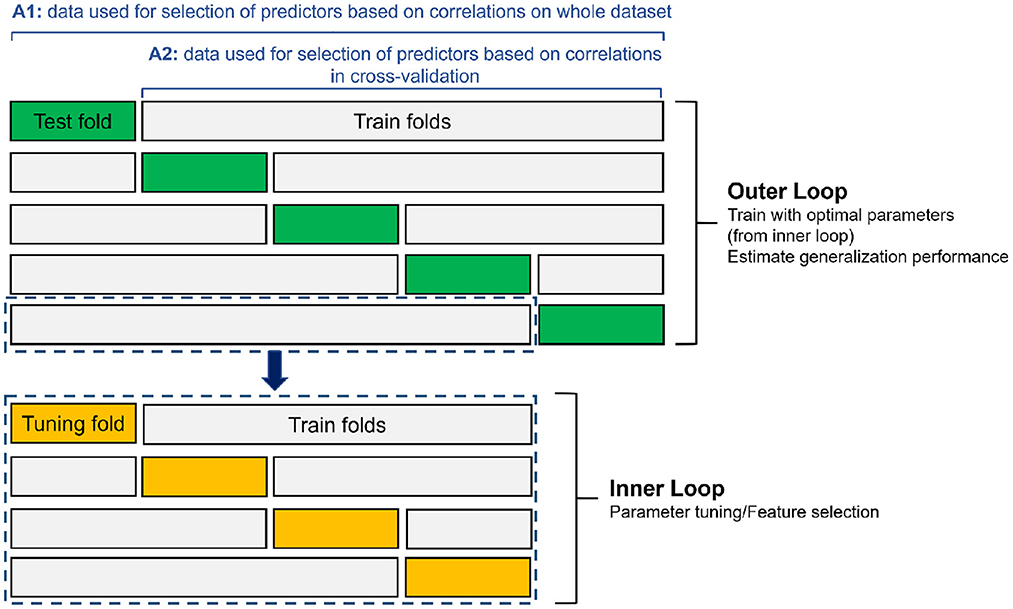
Figure 2. Schematic overview of nested k-fold cross-validation procedure with 5 outer folds and 4 inner folds. A1 refers to the general approach with selecting predictors based on correlations on the whole dataset (1981–2014), while A2 refers to the approach where selection of predictors based on correlations is done only on the training data in the cross-validation procedure (see Section 3.4).
The training data of the outer loop is fed into the inner loop, that splits the data again into training and test (or tuning) data. The inner loop includes predictor selection and hyperparameter optimization procedures that are described in the Supplementary material. Once the optimal set of hyperparameters is found, a final model is constructed using all inner loop data, i.e., the outer loop train data. The performance is then assessed with the never-seen-before test data from the outer loop. For the single-layer neural network, the procedure is slightly different. In the inner loop, a single validation dataset is set apart, because it is not common to use cross-validation in neural networks. Therefore, for the neural networks, we select the best performing model instance of the inner loop—where the tuning set serves as validation set for overfitting—and use this model to estimate the performance on the test data.
In general, the outer loop is used for estimating the performance of a model, while the inner cross-validation is used for tuning the hyperparameters and performing some additional predictor selection. The inner loop can then be seen as a “model selection” phase, where optimal hyperparameters and number of predictors are selected based on performances obtained on the inner loop tuning fold. The selected parameters are then used to construct the model using the training data in the outer loop during a “model training” phase. The trained model is then evaluated in the outer loop using the test data in a “model testing” phase (Varma and Simon, 2006). In each of the outer loop folds, the performance is calculated using the outer loop test data, and those performances obtained over the different folds of the outer loop are subsequently averaged to arrive at an overall performance score, and the standard deviation of the different performances serve as an uncertainty metric. Comparing the outer loop performances of the different modeling methods enables identification of the best method. With nested cross-validation, the test data used in each iteration of the outer loop are completely independent of the data used to optimize the performance of the model, hence it can be seen as a reliable approach for choosing the best modeling method (Varma and Simon, 2006; Wainer and Cawley, 2021).
3.3. Data
Monthly rainfall data comes from the gridded observational Centennial Trends Greater Horn of Africa (CenTrends) precipitation dataset v1.0 [mm/month] (Funk et al., 2015). The data spans the period 1900–2014, at a resolution of 0.1°, and covers the Greater Horn of Africa (–15°S–18°N, 28°E–54°E). Root-zone soil moisture (SMroot) and surface soil moisture (SMsurf) data are acquired from the Global Land Evaporation Amsterdam Model (GLEAM) v3.5a which is available from 1980 with a 0.25° resolution (Miralles et al., 2011; Martens et al., 2017). The Normalized Difference Vegetation Index (NDVI) and Leaf Area Index (LAI) are used to characterize vegetation dynamics. LAI and NDVI data are available from 1981 at a resolution of 0.05° from the National Oceanic and Atmospheric Administration (NOAA) Climate Data Record version 5, and are based on observations from the Advanced Very High Resolution Radiometer (AVHRR) (Vermote, 2019a,b). For the monthly averaged land surface temperature (LST), the Gridded Berkeley Earth Surface Temperature Anomaly Field, available from 1750 with a resolution of 1°, is used (Rohde and Hausfather, 2020).
Global SST data are obtained from the COBE–SST2 product, provided by the NOAA Oceanic and Atmospheric Research (OAR) Earth System Research Laboratory (ESRL) Physical Sciences Laboratory. The dataset has a resolution of 1° and is available over the period 1850–2019 (Hirahara et al., 2014). Monthly data on zonal winds come from the National Centers for Environmental Prediction–National Center for Atmospheric Research (NCEP–NCAR) Climate Data Assimilation System I CDAS–1, and are available from 1949 with a resolution of 2.5° (Kalnay et al., 1996). Zonal winds at 200 and 850 hPa are chosen to consider both the upper troposphere and low level flow. Moreover, ocean–atmosphere oscillation indices are used to diagnose different modes of climate variability; Supplementary Table 2 gives an overview of these indices. They are obtained from NOAA and the Royal Netherlands Meteorological Institute (KNMI).
Finally, retrospective forecast (or hindcast) precipitation data from the European Centre for Medium-Range Weather Forecasts (ECMWF) fifth generation seasonal forecast system (SEAS5, Johnson et al., 2019) are used, not as input, but for comparison. The ECMWF SEAS5 hindcasts consist of 25 ensemble members, at 1° resolution, of which the ensemble average is considered. The hindcast is available from 1981. Datasets have been rescaled to a common 0.25° resolution by bilinear interpolation. Supplementary Table 1 gives an overview of the datasets and their general characteristics.
3.4. Predictor selection
3.4.1. Physics-guided and correlation-based data selection
For a number of predictors (i.e., SMroot, SMsurf, LST, NDVI, LAI, and SST), a physics-guided approach is used for data selection. First, the climatological source regions for precipitation are identified; these are the regions which contribute moisture (through evaporation) to the rainfall occurring in the study region. This is enabled by the use of the Lagrangian FLEXible PARTicle dispersion model FLEXPART (Stohl et al., 2005). Specifically, the FLEXPART model simulations are carried out at a global scale using millions of air parcels which are uniformly distributed throughout the globe and are tracked both in space and time. The following variables are used to force FLEXPART: temperature, specific humidity, horizontal and vertical wind, cloud cover, precipitation, 2-m air temperature, dew-point temperature, sensible and latent heat fluxes, and North/South and West/East surface stress. FLEXPART tracks the location (latitude, longitude, and height) of each parcel and simulates their dynamic and thermodynamic properties (temperature, density, specific humidity). Then, the outputs from FLEXPART are used to construct and evaluate the parcel trajectories, i.e., all air parcels residing over the study region are tracked backward in time and parsed for precipitation in the study region to identify moisture sources in previous time steps and locations. In doing so, all the locations in which the air parcel gains or loses moisture are identified. In this study, the evaluation of air parcel trajectories from the FLEXPART simulations, forced by ERA-Interim reanalysis, are carried out using a recently developed moisture tracking framework (Keune et al., 2022).
The aforementioned steps allow us to delineate the rainfall source regions of the study region, for each of the three MAM months. Once the source regions are determined, predictors are averaged over them. These source regions are shown in Supplementary Figure 1. Atmospheric dynamics such as wind direction play a big role in their location. The dominant easterlies in March are followed by the appearance of low-level flow patterns of the Asian monsoon in April, which show a change in wind and pressure patterns over the Indian Ocean. By May, the low-level flow becomes stronger, with southeasterlies prevailing south of the equator and dominant southwesterlies north of the equator (Nicholson, 2015b). To the authors' knowledge, the use of moisture source regions to delineate and select predictors is novel in the context of seasonal rainfall forecasting.
The set of physics-guided terrestrial and oceanic predictors is combined with the SSTs, zonal winds (200 and 850 hPa) and coupled ocean–atmosphere oscillation indices that are significantly (p < 0.05) correlated with monthly rainfall over the study region. Rainfall data for March, April, and May are correlated with the SST for each lead-time and each pixel, and neighboring significantly correlated pixels are then clustered together. Finally, the averages over these clusters are taken as predictors. For zonal winds at 200 and 850 hPa, the same procedure is repeated. In addition, the climate indices from Supplementary Table 1 are also correlated with MAM rainfall for the 1- to 3-month lead-time and only indices showing significant correlation are retained as predictors. All predictors are standardized using a min–max normalization to rescale them to the same [0–1] range prior to their use in the prediction models (Section 3.1).
3.4.2. Approaches for selection of correlated predictors
The selection of predictors used in data-driven models is typically based on correlations, as outlined above. These correlations are often calculated over all available data, with this approach followed by many studies in seasonal rainfall forecasting (e.g., Block and Rajagopalan, 2007; Diro et al., 2008; Alhamshry et al., 2019). For example, for their prediction of the Ethiopian spring rains, Diro et al. (2008) selected their predictors based on SST correlations over all available years (1969–2003). More recently, Alhamshry et al. (2019) calculated correlations of Ethiopian summer rainfall with global SST fields across the period 1985–2015 and used the result to select predictors. Following this, they trained an Elman recurrent neural network using 1985–2000 data, and optimized their model for 2001–2015, eventually defining their final optimization as the best fit for the whole period 1985–2015. Multiple other studies have used this approach, both in the eastern Africa region (e.g., Block and Rajagopalan, 2007; Nicholson, 2014b, 2015b), as well as elsewhere (e.g., Singhrattna et al., 2005). This commonly-used predictor selection approach is also explored in this study and referred to as A1. The problem with A1 is that it may lead to biased performance measures, as the test set is not fully independent.
In the field of machine learning, it is known that selecting variables within the cross-validation procedure, instead of prior to it, is of utmost importance, and doing otherwise may yield optimistically biased predictions (Krstajic et al., 2014). Therefore, a more “statistically correct” approach is also examined in this study, and further referred to as A2. In A2, and just like in A1, for each fold of the five outer cross-validation loops, a subset of good predictors is found that show strong enough correlation using all samples. However, unlike in A1, the test data are excluded in the selection of predictors. As a consequence, in A2, significantly correlated SSTs, winds and climate indices are selected and clustered in the outer cross-validation procedure, as also shown in Figure 2. In other words, instead of using all data (1981–2014) to select correlation-based predictors (e.g., the SST correlations), the correlations and the clustering are done excluding test years. This predictor set is subsequently merged with the physics-guided input data. The set of predictors, selected in the outer loop, is then further used to fit the models in the inner loop and to eventually evaluate performance against the test set. For every fold of the outer loop, the set of predictors may thus be different. Selecting variables within the cross-validation procedure is not necessary for the physics-guided predictors, as those are independent because they are not selected based on correlations with the long rains. By using both approaches, a comparison between them can be made, and enables the discussion of the effect of selecting predictors based on correlations prior to cross-validation for seasonal forecasting in the study area. See Supplementary material for the pseudocode of the predictor selection.
4. Results
4.1. Performance of data-driven models vs. dynamic weather hindcasts
First, the A1 approach, in which the entire time series is used to preselect correlated predictors, is evaluated. Figure 3 provides an overview of the performance of the different data-driven models when following this A1 approach, and it indicates a good predictive skill, comparable to dynamical weather hindcasts (SEAS5), and frequently superior. Figure 3A shows time series of cumulative precipitation for MAM at a 1-month lead-time. Even some of the more extreme years are reasonably well-hindcasted. The Kling–Gupta efficiency (KGE) metric is used to compare the performance of the different models in Figure 3B. KGE combines the correlation coefficient (r), bias (β), and ratio of the standard deviations (α) by computing the Euclidean distance (ED) of the three components from its ideal point (Gupta et al., 2009); KGE-values > −0.41 indicate some skill compared to using the climatological mean as hindcast (Knoben et al., 2019). For a 1-month lead-time, the highest KGE values for the month of March are found for using lasso models (KGE = 0.27), while ridge regressions perform best in April (0.30) and May (0.60). For 2- and 3-month lead-times, the performances are slightly worse, as expected, but the lasso and ridge regression models still maintain a high level of predictability, consistently outperforming the dynamical hindcasts. Supplementary Table 2 illustrates the partitioning of the KGE values into its three different components (r, β, α). The skill demonstrated by the data-driven hindcasts in terms of correlation coefficient to the observations (best model frequently r> 0.4) is comparable to the values reported by previous studies in eastern Africa that use this conventional A1 approach for predictor selection (Nicholson, 2015b; Alhamshry et al., 2019).
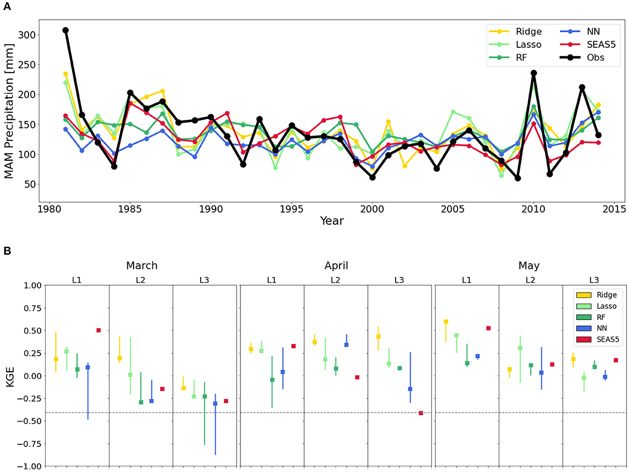
Figure 3. Performance of the conventional A1 approach for predictor selection. (A) Time series of observations and hindcasts of the nested cross-validation procedure of all modeling methods for MAM at a 1-month lead-time representing the first approach where correlation-based predictors were done on the whole dataset (A1). (B) Median and interquartile ranges illustrating the Kling–Gupta Efficiency (KGE) performances of the cross-validation procedure for the four data-driven models and the dynamical hindcast at all lead-times (L1–L3). RF and NN refer to the random forest and the single-layer neural network, respectively. KGE-values > −0.41 (see discontinuous line) indicate some skill compared to using the climatological mean as hindcast.
4.2. On the pitfall of using correlation-based predictors
As mentioned in Section 3.4, the main issue with the conventional (A1) approach is that its verification sample is not fully independent, resulting in the forecast skill being optimistically biased (Hastie et al., 2009). Therefore, the analysis is repeated using the statistically correct A2 approach. As noted in Section 3.4, in A2, the correlations and clustering used to preselect predictor variables were computed excluding the years used for testing. Figure 4 shows poor results for the A2 approach in terms of predicted performance. Extreme years are no longer adequately represented. While the performance of random forests, lasso regression and neural networks at 1-, 2-, and 3-month lead-times (respectively) is comparatively superior to the other data-driven approaches, the performance of SEAS5 is still typically superior to all of them. To fully understand the origin of the low performance for A2, the KGE is decomposed into its three components (r, α, and β) in Supplementary Table 2. The correlation (r) differs greatly between the two approaches and rarely exceeds 0.2 in A2, being sometimes even negative, while the values of A1 are in line with those in literature (Nicholson, 2015b; Alhamshry et al., 2019). For A2, the performance of the data-driven hindcasts drops significantly below that of SEAS5 (Figure 4B). The bias (β) is not responsible for the low KGE values for A2, which fluctuate around the mean. The reason for the low KGE of A2 is the low correlation (r) in hindcasted vs. observed rainfall, but also the low variability (α). Overall, extremes are almost never captured with the A2 approach with hindcasts showing only a slight deviation from the mean, and hence with peaks and lows being under- and overestimated, respectively. Comparing the statistics shown in Figure 3B for the A1 approach, it is clear that A1 performs unrealistically well because of the dependency between the predictor selection and testing samples. This hides a problem of overfitting in the conventional A1 approach, which would result in low predictability for the years outside the pool of data used in predictor selection, misrepresenting the true value of the models for real-world forecasting.
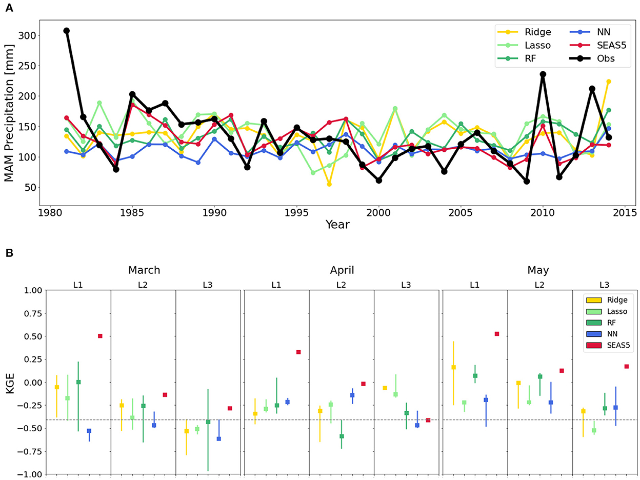
Figure 4. Performance of the A2 approach for predictor selection where independent test data is used that is not employed in the preselection of correlated predictors. (A) Time series of observations and hindcasts of the nested cross-validation procedure of all modeling methods for MAM at a 1-month lead-time representing the second approach where correlations are performed inside the cross-validation loop, excluding the years used for testing (A2). (B) Median and interquartile ranges illustrating the Kling–Gupta Efficiency (KGE) performances of the cross-validation procedure for the four data-driven models and the dynamical hindcast at all lead-times (L1–L3). RF and NN refer to the random forest and the single-layer neural network, respectively. KGE-values > −0.41 (see discontinuous line) indicate some skill compared to using the climatological mean as hindcast.
5. Discussion
Our results point to a serious issue affecting many previous studies which evaluate statistical seasonal climate forecasting. If predictor selection is not carried out properly, and performed based on correlations over the entire data record, overly optimistic predictive skill is expected. Therefore, the reported level of forecast skill in data-driven methods is often significantly overestimated. Future studies must consider this potential pitfall and explore new avenues to increase predictability without overfitting. The overfitting underlying the A1 approach is evidenced once more by Figure 5, which illustrates how the temporal correlation clusters between pixel SST and the study region precipitation differ when looking at slightly different periods for the calculation of these correlations. Purely coincidental correlations occur due to the large number of pixels and the limited temporal granularity, and it falsely increases the predictive power of the models that use these regions as predictors when the test data is also included in the time series used to compute these correlations. If the SSTs from these correlation clusters were selected as predictors in the data-driven models, the spurious nature of these correlations would indicate that they do not necessarily reflect any underlying physical process linking the SSTs and the region's rainfall. This makes the SSTs in these regions uninformative when it comes to operational forecast systems that go beyond the historical observational period. In larger datasets, it could be that the significant correlations do not change as much when taking a part of the data out as a test set, which could result in correlation clusters that are more consistent. The difference in outcome between the two approaches would then also be smaller. Nonetheless, it is important to consider that the use of longer time periods may mean historical correlations are unrepresentative of present times due to non-stationarity in climate teleconnections (Weisheimer et al., 2017).

Figure 5. Maps with clusters of significant correlations (p < 0.05) of SSTs with May rainfall at a 1-month lead-time, indicated in blue for the five folds and over the whole available period.
Although recent work improved in investigating sources of interannual variability, the long rains in the Horn of Africa remain difficult to predict at seasonal scales (Vellinga and Milton, 2018; MacLeod, 2019; Finney et al., 2020). This is particularly the case during the long rains, and it is evidenced by the low predictability as the lead-time increases. Therefore, the low predictability achieved when using the statistically correct approach (A2) is not totally unexpected. Nonetheless, there are several means to improve machine-learning predictions of long rains upon what is presented in this study. First, with only 34 years of data available, the partitioning into train, test, and validation yields limited samples, which hinders the accuracy of the hindcasts. In the case of neural networks this is particularly important, and they should be used with larger datasets to fully capture the complex interactions. Second, the hindcasting was done for the study area as a whole, delineated as a region of homogeneous bimodal annual rainfall seasonality. However, during the long rains, the amount of rain falling over the area still differs; the northeastern tip is drier than the southwestern part (Figure 1A). Third, the predictor selection based on correlations used linear correlations (for SSTs and zonal winds), while the random forest and neural network algorithm can capture possible non-linear trends as well. Possible SST and wind clusters with a non-linear relationship with rainfall might thus be missing in the predictor set. If longer time series were used for training, the higher probability of non-stationary and non-linear changes should be considered in the predictions and in the predictor selection. Finally, the added value of using physics-guided input data as predictors could not be determined given the low predictability of the target variable. This approach should be further studied in the future, and is expected to have a larger potential in regions with continental-origin rainfall, in which the land state upwind may have a large influence on the precipitation occurrence in the downwind region (Miralles et al., 2019).
6. Conclusion
In this study, seasonal rainfall hindcasting in the Horn of Africa drylands was performed using four data-driven modeling methods: ridge and lasso linear regression, random forests, and single-layer neural networks. The performance of each of the methods was assessed using nested k-fold cross-validation. The three long rain months (March, April, and May) were studied separately and hindcasts were done for lags of 1–3 months. Significantly correlated clusters of SSTs, zonal winds, and coupled ocean–atmosphere oscillation indices were selected as predictor data. These were merged with terrestrial and oceanic variables which were averaged over the region sourcing moisture during each of the long rain months. The source regions were obtained through Lagrangian transport modeling.
Our findings reveal a pitfall in the conventional approach of selecting predictors as predictors based on correlations to the target variable, without testing the performance using independent data. This conventional approach yielded prediction scores that indicated a high performance of the data-driven models—particularly ridge and lasso regressions—compared to the performance of dynamical hindcasts. However, comparison with a more statistically correct approach wherein the predictor selection was done inside the cross-validation loop on the training data (and thus maintaining the test and predictor selection as independent samples) demonstrated a tendency toward overfitting by the conventional approach. When testing and selecting predictors in independent samples, all four modeling methods performed poorly in their prediction of long rains, especially at 2- or 3-month lead-times, and worse than the dynamical hindcasts. The results in this study should not discourage future applications of machine learning for rainfall forecasting in the region, but rather be seen as a note of caution to prevent the (frequently done) selection of predictors based on correlations to the entire observational period. That gives optimistically biased results that are not indicative of the true power in operational forecast systems that aim to predict beyond the historical period.
Furthermore, our results also confirm that seasonal rainfall forecasting in the Horn of Africa dryland region is particularly challenging, certainly during the long rain season, and particularly for extreme values. The lack of forecast skill could be attributed to several factors, such as the lack of understanding of long rain interannual variability, limitations in record length, and the consideration of a large study area as a homogeneous geographical unit. Further research should continue focusing on pinpointing sources of predictability during the long rains and improving process understanding in order to inform predictor selection (Vellinga and Milton, 2018). Furthermore, other suggestions include exploring more advanced deep learning techniques such as convolutional or recurrent neural networks, and hybrid techniques combining dynamical and data-driven approaches.
Data availability statement
The raw data supporting the conclusions of this article will be made available by the authors, without undue reservation.
Author contributions
AK and DGM conceived the study. VMHD, AK, DGM, and WW designed the experiments. VMHD conducted the analysis. VMHD and DGM wrote the paper, with contributions from all coauthors. All authors contributed to the interpretation and discussion of the results.
Funding
This study was funded by the European Union Horizon 2020 Programme (DOWN2EARTH, 869550).
Acknowledgments
DGM acknowledges support from the European Research Council (DRY–2–DRY, 715254). WW acknowledges funding from the Flemish Government under the Onderzoeksprogramma Artificiële Intelligentie (AI) Vlaanderen programme.
Conflict of interest
The authors declare that the research was conducted in the absence of any commercial or financial relationships that could be construed as a potential conflict of interest.
Publisher's note
All claims expressed in this article are solely those of the authors and do not necessarily represent those of their affiliated organizations, or those of the publisher, the editors and the reviewers. Any product that may be evaluated in this article, or claim that may be made by its manufacturer, is not guaranteed or endorsed by the publisher.
Supplementary material
The Supplementary Material for this article can be found online at: https://www.frontiersin.org/articles/10.3389/frwa.2022.1053020/full#supplementary-material
References
Adloff, M., Singer, M. B., MacLeod, D. A., Michaelides, K., Mehrnegar, N., Hansford, F.unk, C., et al. (2022). Sustained water storage in Horn of Africa drylands dominated by seasonal rainfall extremes. Environ. Res. Lett. 49, e2022GL099299. doi: 10.1029/2022GL099299
Alhamshry, A., Fenta, A. A., Yasuda, H., Shimizu, K., and Kawai, T. (2019). Prediction of summer rainfall over the source region of the Blue Nile by using teleconnections based on sea surface temperatures. Theoret. Appl. Climatol. 137, 3077–3087. doi: 10.1007/s00704-019-02796-x
Bauer, P., Thorpe, A., and Brunet, G. (2015). The quiet revolution of numerical weather prediction. Nature 525, 47–55. doi: 10.1038/nature14956
Behera, S. K., Luo, J.-J., Masson, S., Delecluse, P., Gualdi, S., Navarra, A., et al. (2005). Paramount impact of the Indian Ocean dipole on the east african short rains: a CGCM study. J. Clim. 18, 4514–4530. doi: 10.1175/JCLI3541.1
Biau, G., and Scornet, E. (2016). A random forest guided tour. Test 25, 197–227. doi: 10.1007/s11749-016-0481-7
Block, P., and Rajagopalan, B. (2007). Interannual variability and ensemble forecast of Upper Blue Nile Basin Kiremt season precipitation. J. Hydrometeorol. 8, 327–343. doi: 10.1175/JHM580.1
Bochenek, B., and Ustrnul, Z. (2022). Machine learning in weather prediction and climate analyses—applications and perspectives. Atmosphere 13, 180. doi: 10.3390/atmos13020180
Camberlin, P., and Philippon, N. (2002). The East African March-May rainy season: associated atmospheric dynamics and predictability over the 1968-97 period. J. Clim. 15, 1002–1019. doi: 10.1175/1520-0442(2002)015<1002:TEAMMR>2.0.CO;2
Cohen, J., Coumou, D., Hwang, J., Mackey, L., Orenstein, P., Totz, S., et al. (2019). S2S reboot: an argument for greater inclusion of machine learning in subseasonal to seasonal forecasts. Wiley Interdiscipl. Rev. Clim. Change 10, e00567. doi: 10.1002/wcc.567
Davies, R. (2021). Ethiopia–Deadly Flash Floods in Addis Ababa. Floodlist. Available online at: https://floodlist.com/africa/ethiopia-floods-addis-ababa-august-2021 (accessed December 20, 2021).
Dewitte, S., Cornelis, J. P., Müller, R., and Munteanu, A. (2021). Artificial intelligence revolutionises weather forecast, climate monitoring and decadal prediction. Remote Sens. 13, 3209. doi: 10.3390/rs13163209
Diro, G. T., Black, E., and Grimes, D. (2008). Seasonal forecasting of Ethiopian spring rains. Meteorol. Appl. 15, 73–83. doi: 10.1002/met.63
Finney, D. L., Marsham, J. H., Walker, D. P., Birch, C. E., Woodhams, B. J., Jackson, L. S., et al. (2020). The effect of westerlies on East African rainfall and the associated role of tropical cyclones and the Madden-Julian Oscillation. Q. J. R. Meteorol. Soc. 146, 647–664. doi: 10.1002/qj.3698
Funk, C., Harrison, L., Shukla, S., Pomposi, C., Galu, G., Korecha, D., et al. (2018). Examining the role of unusually warm indo-pacific sea-surface temperatures in recent African droughts. Q. J. R. Meteorol. Soc. 144, 360–383. doi: 10.1002/qj.3266
Funk, C., Nicholson, S. E., Landsfeld, M., Klotter, D., Peterson, P., and Harrison, L. (2015). The centennial trends greater Horn of Africa precipitation dataset. Sci. Data 2, 1–17. doi: 10.1038/sdata.2015.50
Funk, C., Shukla, S., Thiaw, W. M., Rowland, J., Hoell, A., McNally, A., et al. (2019). Recognizing the famine early warning systems network: over 30 years of drought early warning science advances and partnerships promoting global food security. Bull. Am. Meteorol. Soc. 100, 1011–1027. doi: 10.1175/BAMS-D-17-0233.1
Gupta, H. V., Kling, H., Yilmaz, K. K., and Martinez, G. F. (2009). Decomposition of the mean squared error and NSE performance criteria: implications for improving hydrological modelling. J. Hydrol. 377, 80–91. doi: 10.1016/j.jhydrol.2009.08.003
Hastie, T., Tibshirani, R., and Friedman, J. H. (2009). The Elements of Statistical Learning: Data Mining, Inference, and Prediction, Vol. 2. New York: Springer. doi: 10.1007/978-0-387-84858-7
He, S., Li, X., DelSole, T., Ravikumar, P., and Banerjee, A. (2021). “Sub-seasonal climate forecasting via machine learning: challenges, analysis, and advances,” in Proceedings of the AAAI Conference on Artificial Intelligence, 169–177. doi: 10.1609/aaai.v35i1.16090
Hirahara, S., Ishii, M., and Fukuda, Y. (2014). Centennial-scale sea surface temperature analysis and its uncertainty. J. Clim. 27, 57–75. doi: 10.1175/JCLI-D-12-00837.1
Johnson, S. J., Stockdale, T. N., Ferranti, L., Balmaseda, M. A., Molteni, F., Magnusson, L., et al. (2019). SEAS5: the new ECMWF seasonal forecast system. Geosci. Model Dev. 12, 1087–1117. doi: 10.5194/gmd-12-1087-2019
Kalnay, E., Kanamitsu, M., Kistler, R., Collins, W., Deaven, D., Gandin, L., et al. (1996). The NCEP/NCAR 40-year reanalysis project. Bull. Am. Meteorol. Soc. 77, 437–471. doi: 10.1175/1520-0477(1996)077<0437:TNYRP>2.0.CO;2
Keune, J., Schumacher, D. L., and Miralles, D. G. (2022). A unified framework to estimate the origins of atmospheric moisture and heat using Lagrangian models. Geosci. Model Dev. 15, 1875–1898. doi: 10.5194/gmd-15-1875-2022
Knoben, W. J. M., Freer, J. E., and Woods, R. A. (2019). Inherent benchmark or not? Comparing Nash-Sutcliffe and Kling-Gupta efficiency scores. Hydrol. Earth Syst. Sci. 23, 4323–4331. doi: 10.5194/hess-23-4323-2019
Krstajic, D., Buturovic, L. J., Leahy, D. E., and Thomas, S. (2014). Cross-validation pitfalls when selecting and assessing regression and classification models. J. Cheminform. 6, 1–15. doi: 10.1186/1758-2946-6-10
Lang, A. L., Pegion, K., and Barnes, E. A. (2020). Introduction to special collection: “bridging weather and climate: subseasonal-to-seasonal (S2S) prediction”. J. Geophys. Res. Atmos. 125, e2019JD031833. doi: 10.1029/2019JD031833
MacLeod, D. (2019). Seasonal forecasts of the East African long rains: insight from atmospheric relaxation experiments. Clim. Dyn. 53, 4505–4520. doi: 10.1007/s00382-019-04800-6
MacLeod, D., Graham, R., O'Reilly, C., Otieno, G., and Todd, M. (2021). Causal pathways linking different flavours of enso with the greater horn of africa short rains. Atmos. Sci. Lett. 22, e1015. doi: 10.1002/asl.1015
Manatsa, D., and Behera, S. K. (2013). On the epochal strengthening in the relationship between rainfall of East Africa and IOD. J. Clim. 26, 5655–5673. doi: 10.1175/JCLI-D-12-00568.1
Mariotti, A., Baggett, C., Barnes, E. A., Becker, E., Butler, A., Collins, D. C., et al. (2020). Windows of opportunity for skillful forecasts subseasonal to seasonal and beyond. Bull. Am. Meteorol. Soc. 101, E608–E625. doi: 10.1175/BAMS-D-18-0326.1
Martens, B., Miralles, D. G., Lievens, H., Van Der Schalie, R., De Jeu, R. A., Fernández-Prieto, D., et al. (2017). GLEAM v3: Satellite-based land evaporation and root-zone soil moisture. Geosci. Model Dev. 10, 1903–1925. doi: 10.5194/gmd-10-1903-2017
Mekanik, F., Imteaz, M., Gato-Trinidad, S., and Elmahdi, A. (2013). Multiple regression and Artificial Neural Network for long-term rainfall forecasting using large scale climate modes. J. Hydrol. 503, 11–21. doi: 10.1016/j.jhydrol.2013.08.035
Merryfield, W. J., Baehr, J., Batté, L., Becker, E. J., Butler, A. H., Coelho, C. A., et al. (2020). Subseasonal to decadal prediction: filling the weather-climate gap. Bull. Am. Meteorol. Soc. 101, 767–770. doi: 10.1175/BAMS-D-19-0037.A
Miralles, D. G., Gentine, P., Seneviratne, S. I., and Teuling, A. J. (2019). Land-atmospheric feedbacks during droughts and heatwaves: state of the science and current challenges. Ann. N. Y. Acad. Sci. 1436, 19–35. doi: 10.1111/nyas.13912
Miralles, D. G., Holmes, T., De Jeu, R., Gash, J., Meesters, A., and Dolman, A. (2011). Global land-surface evaporation estimated from satellite-based observations. Hydrol. Earth Syst. Sci. 15, 453–469. doi: 10.5194/hess-15-453-2011
Mwale, D., and Gan, T. Y. (2005). Wavelet analysis of variability, teleconnectivity, and predictability of the September-November East African rainfall. J. Appl. Meteorol. 44, 256–269. doi: 10.1175/JAM2195.1
Nayak, D. R., Mahapatra, A., and Mishra, P. (2013). A survey on rainfall prediction using artificial neural network. Int. J. Comput. Appl. 72, 32–40. doi: 10.5120/12580-9217
Nicholson, S. E. (2014a). A detailed look at the recent drought situation in the Greater Horn of Africa. J. Arid Environ. 103, 71–79. doi: 10.1016/j.jaridenv.2013.12.003
Nicholson, S. E. (2014b). The predictability of rainfall over the Greater Horn of Africa. Part I: Prediction of seasonal rainfall. J. Hydrometeorol. 15, 1011–1027. doi: 10.1175/JHM-D-13-062.1
Nicholson, S. E. (2015a). Long-term variability of the east African “short rains” and its links to large-scale factors. Int. J. Climatol. 35, 3979–3990. doi: 10.1002/joc.4259
Nicholson, S. E. (2015b). The predictability of rainfall over the Greater Horn of Africa. Part II: Prediction of monthly rainfall during the long rains. J. Hydrometeorol. 16, 2001–2012. doi: 10.1175/JHM-D-14-0138.1
Ntale, H. K., Gan, T. Y., and Mwale, D. (2003). Prediction of East African seasonal rainfall using simplex canonical correlation analysis. J. Climate 16, 2105–2112. doi: 10.1175/1520-0442(2003)016<2105:POEASR>2.0.CO;2
Reichstein, M., Camps-Valls, G., Stevens, B., Jung, M., Denzler, J., Carvalhais, N., et al. (2019). Deep learning and process understanding for data-driven Earth system science. Nature 566, 195–204. doi: 10.1038/s41586-019-0912-1
Rohde, R. A., and Hausfather, Z. (2020). The Berkeley Earth land/ocean temperature record. Earth Syst. Sci. Data 12, 3469–3479. doi: 10.5194/essd-12-3469-2020
Scher, S. (2018). Toward data-driven weather and climate forecasting: approximating a simple general circulation model with deep learning. Geophys. Res. Lett. 45, 12–616. doi: 10.1029/2018GL080704
Schultz, M. G., Betancourt, C., Gong, B., Kleinert, F., Langguth, M., Leufen, L. H., et al. (2021). Can deep learning beat numerical weather prediction? Philos. Trans. R. Soc. A 379, 20200097. doi: 10.1098/rsta.2020.0097
Singhrattna, N., Rajagopalan, B., Clark, M., and Krishna Kumar, K. (2005). Seasonal forecasting of Thailand summer monsoon rainfall. Int. J. Climatol. J. R. Meteorol. Soc. 25, 649–664. doi: 10.1002/joc.1144
Slim, H. (2012). IASC Real-Time Evaluation of the Humanitarian Response to the Horn of Africa Drought Crisis in Somalia, Ethiopia and Kenya. Available online at: reliefweb.int/sites/reliefweb.int/files/resources/RTE_HoA_SynthesisReport_FINAL.pdf
Stohl, A., Forster, C., Frank, A., Seibert, P., and Wotawa, G. (2005). Technical note: the Lagrangian particle dispersion model flexpart version 6.2. Atmos. Chem. Phys. 5, 2461–2474. doi: 10.5194/acp-5-2461-2005
Tibshirani, R. (1996). Regression shrinkage and selection via the lasso. J. R. Stat. Soc. Ser. B Methodol. 58. 267–288. doi: 10.1111/j.2517-6161.1996.tb02080.x
UN OCHA (2022). Horn of Africa Drought: Humanitarian Key Messages. Available online at: https://reliefweb.int/sites/reliefweb.int/files/resources/20220422_RHPT_KeyMessages_HornOfAfricaDrought.pdf (accessed April 26, 2022).
Varma, S., and Simon, R. (2006). Bias in error estimation when using cross-validation for model selection. BMC Bioinformatics 7, 91. doi: 10.1186/1471-2105-7-91
Vellinga, M., and Milton, S. F. (2018). Drivers of interannual variability of the east african “long rains”. Q. J. R. Meteorol. Soc. 144, 861–876. doi: 10.1002/qj.3263
Vermote, E. (2019a). NOAA Climate Data Record (CDR) of AVHRR Leaf Area Index (LAI) and Fraction of Absorbed Photosynthetically Active Radiation (FAPAR). Version 5.
Vermote, E. (2019b). NOAA Climate Data Record (CDR) of AVHRR Normalized Difference Vegetation Index (NDVI). Version 5.
Wainer, J., and Cawley, G. (2021). Nested cross-validation when selecting classifiers is overzealous for most practical applications. Expert Syst. Appl. 182, 115222. doi: 10.1016/j.eswa.2021.115222
Weisheimer, A., Schaller, N., O'Reilly, C., MacLeod, D. A., and Palmer, T. (2017). Atmospheric seasonal forecasts of the twentieth century: multi-decadal variability in predictive skill of the winter North Atlantic Oscillation (NAO) and their potential value for extreme event attribution. Q. J. R. Meteorol. Soc. 143, 917–926. doi: 10.1002/qj.2976
Keywords: Horn of Africa, seasonal rainfall prediction, machine learning, long rains, drylands
Citation: Deman VMH, Koppa A, Waegeman W, MacLeod DA, Bliss Singer M and Miralles DG (2022) Seasonal prediction of Horn of Africa long rains using machine learning: The pitfalls of preselecting correlated predictors. Front. Water 4:1053020. doi: 10.3389/frwa.2022.1053020
Received: 24 September 2022; Accepted: 22 November 2022;
Published: 08 December 2022.
Edited by:
Ibrahim Demir, The University of Iowa, United StatesReviewed by:
Salim Heddam, University of Skikda, AlgeriaGuoqiang Tang, University of Saskatchewan, Canada
Copyright © 2022 Deman, Koppa, Waegeman, MacLeod, Bliss Singer and Miralles. This is an open-access article distributed under the terms of the Creative Commons Attribution License (CC BY). The use, distribution or reproduction in other forums is permitted, provided the original author(s) and the copyright owner(s) are credited and that the original publication in this journal is cited, in accordance with accepted academic practice. No use, distribution or reproduction is permitted which does not comply with these terms.
*Correspondence: Diego G. Miralles, RGllZ28uTWlyYWxsZXNAVUdlbnQuYmU=