 Parul Vinze
 Mohd. Farooq Azam
- Department of Civil Engineering, Indian Institute of Technology Indore, Indore, MP, India
Snowmelt runoff plays a major role in the glacierized and snow-covered basins in the western Himalaya. Modeling is the most helpful tool to quantify snowmelt contribution in mountainous rivers. However, the model calibration is very difficult because of the scarcity of ground observations in the Himalaya. We applied snowmelt runoff model (SRM) in a reference catchment of Chhota Shigri Glacier in the Chandra-Bhaga Basin, western Himalaya. Three model parameters [temperature lapse rate and recession coefficients (x and y)] among the nine model parameters were constrained using extensive field observations while initial values of other parameters were adopted from previous studies and calibrated, and the model was calibrated and validated against the observed discharge data. The daily discharge was simulated over 2003–2018 for both Chhota Shigri Catchment and Chandra-Bhaga Basin using snow cover area (SCA), precipitation, and temperature as inputs. The simulated mean annual discharges were 1.2 ± 0.2 m3/s and 55.9 ± 12.1 m3/s over 2003–2018 for Chhota Shigri Catchment and Chandra-Bhaga Basin, respectively. The reconstructed discharge was mainly controlled by summer temperature and summer SCA in the Chhota Shigri Catchment and summer SCA and summer precipitation in the Chandra-Bhaga Basin. The decadal comparison showed an increase (11% and 9%) and early onset (10 days and 20 days) of maximum monthly discharge over 2011–2018 compared to 2003–2010 in both catchment and basin scales. The model output is almost equally sensitive to the “degree day factor” and “runoff coefficient for snow” in the Chhota Shigri Catchment and most sensitive to the “runoff coefficient for snow” in the Chandra-Bhaga Basin. Though the SRM parameters were constrained/calibrated in a data-plenty reference catchment of Chhota Shigri Glacier, their application resulted in large discharge overestimation at the basin scale and were not transferable in the same basin i.e., Chandra-Bhaga Basin. Extreme care must be taken while using SRM parameters from other basins.
1. Introduction
The Himalaya-Karakoram (HK) Range also known as the Water Tower of Asia contains huge storage of water in the form of large number of glaciers, snow cover, and permafrost. The HK Range contributes to the discharge of major river systems like the Ganga, Indus, and Brahmaputra in the form of snow and glacier melt (Immerzeel et al., 2020; Azam et al., 2021). Due to global and regional warming (Banerjee and Azam, 2016; Pörtner et al., 2022), glaciers in the Himalaya have been losing their mass at an accelerating rate since 2000 (Brun et al., 2017; Azam et al., 2018; Bolch et al., 2019; Maurer et al., 2019; Shean et al., 2020) which resulted in the increased discharge volume in these rivers (Lutz et al., 2014; Azam et al., 2021). The latest IPCC 6th assessment report stated that global warming will reach or exceed 1.5°C above the pre-industrial level in the next two decades (Pörtner et al., 2022). This temperature rise would result in decreasing snow cover, retreating glaciers, changes in river seasonality, and higher river discharge, which can be the main cause of different hazards like floods, landslides, etc. The discharge from snow-covered and glacierized catchments mainly involves contributions from snowmelt, glacier melt, baseflow, and rainfall-runoff. The snowmelt contribution to the river discharge is large in the Indus Basin (Karakoram and western Himalaya) because it receives a major portion of annual precipitation in the form of snow during winter that provides snowmelt discharge during summer (Azam et al., 2021). Conversely, in the Ganga and Brahmaputra basins (central and eastern Himalaya), the total discharge is dominated by the monsoonal rains as these basins receive the maximum precipitation from Indian Summer Monsoon during summer. A study by Bookhagen and Burbank (2010) found a pronounced contribution of snowmelt to total discharge in the Karakoram and western Himalaya as compared to the central and eastern Himalaya. Since snowmelt plays a significant role in the discharge of Himalayan rivers, it must be accurately estimated using suitable methods and modeling techniques with appropriate model parameters and inputs.
Snowmelt runoff modeling has usually been done using temperature-index or energy balance models. Whereas, the temperature-index models are simple and need fewer input data, the energy balance models are sophisticated and require plenty of meteorological data (Hock, 2003; Shea et al., 2015; Srivastava and Azam, 2022). In the Himalayan region due to the adverse situations induced by steep terrain, harsh climatic conditions, and remote access to the high-altitude regions (Vishwakarma et al., 2022), the monitoring of meteorological data is very difficult hence the application of energy balance models is very challenging. The temperature-index models follow the degree-day approach to estimate the melt (Hock, 2003). The snowmelt runoff model (SRM), based on the degree-day approach, is developed to simulate the daily discharge under changing climate from mountain basins where the snowmelt plays an important role (Martinec et al., 2007). SRM has widely been applied and tested on more than 100 basins of varying areas by different agencies (Martinec et al., 2007) to simulate and forecast the daily discharge from the glacierized catchments in different mountain ranges. This model uses long-term meteorological and remotely sensed snow cover data as basic input for generating discharge at the outlet (Martinec et al., 2007; Tahir et al., 2011).
The SRM has also been applied in several studies for simulating daily discharge in the HK range (Immerzeel et al., 2009; Bookhagen and Burbank, 2010; Jain et al., 2010; Tahir et al., 2011; Panday et al., 2014). As snow cover area (SCA) has also been included in SRM for the simulation of daily discharge hence it can also be applied to study the impact of reduced snow cover on discharge (Immerzeel et al., 2009). For the regions where only the gridded precipitation and temperature dataset are available, SRM performs as an efficient tool for snowmelt runoff modeling. Several studies tested this model with gridded datasets of temperature and precipitation like APHRODITE, TRMM, etc. (Immerzeel et al., 2009; Bookhagen and Burbank, 2010; Tahir et al., 2011; Zhang et al., 2014). Jain et al. (2010) applied SRM in the Sutlej Basin (western Himalaya) and found that seasonally varied temperature lapse rate increases the efficiency of the SRM, which shows the model is sensitive to the temperature lapse rate parameter. Applying the SRM in the Hunza River Basin (Karakoram), Tahir et al. (2011) demonstrated that SRM, using SCA as an input, is relatively less sensitive to the precipitation input hence its efficiency is not hampered in high-altitude catchments where the precipitation measurements contain large uncertainties. The high accuracy of SRM runoff simulation in the Astore River Basin part of the Indus Basin showed that the SRM is suitable for the runoff forecast and water resource management (Butt and Bilal, 2011). Tahir et al. (2019) applied SRM in the Shyok River Basin (Karakoram) to assess the snowmelt discharge under climate change scenarios and found that the SRM is an efficient tool to simulate the snowmelt discharge in data-scarce regions. SRM was also applied for future runoff simulation under different climate scenarios in the Astore Basin (Karakoram) and Hunza Basin (western Himalaya) and resulted in an effective tool for runoff forecast (Hayat et al., 2019). Different SCA products from MODIS like MOD10A2 and MOD10C2 have been widely used and shown to perform well in several studies (Immerzeel et al., 2009; Bookhagen and Burbank, 2010; Tahir et al., 2011; Panday et al., 2014; Zhang et al., 2014; Haq et al., 2020, 2021a).
Available studies suggested that the SRM is a simple and efficient model which can be applied in high-altitude catchments due to its less sensitivity toward the precipitation input, flexibility with the gridded dataset, and SCA integration in the modeling scheme. Further, SRM requires a set of parameters that depends on the catchment area characteristics and the climatic conditions in the catchment. Due to the lack of information about the observed parameters in the Himalayan catchments, these parameters are being calibrated with the observed discharge or have been taken from previous studies (Butt and Bilal, 2011; Tahir et al., 2011; Panday et al., 2014; Hayat et al., 2019). But since model parameters play a vital role in model calibration to constrain the model to overfit, they require special attention in snowmelt runoff modeling.
In the present study, we applied SRM to reconstruct the daily discharge from a small catchment of Chhota Shigri Glacier [34.7 km2; volume of Chhota Shigri glacier is 1.69 km3 (Haq et al., 2021b)] and Chandra-Bhaga Basin (including Chhota Shigri Catchment) having a large area (~4,108 km2) up to the point of confluence of Chandra and Bhaga rivers at Tandi village in Himachal Pradesh. We simulated the daily discharge for the period of 2003–2018 for both the study regions: Chhota Shigri Catchment and Chandra-Bhaga Basin. We selected small and large scales to check the performance of SRM for snowmelt runoff modeling at catchment scale and basin-scale having distinct characteristics. The main objectives for this study are (a) To reconstruct the daily discharge separately for the Chhota Shigri Catchment and Chandra-Bhaga Basin and assess the discharge pattern characteristics, (b) to analyze the model sensitivity to all input parameters in SRM, and (c) to assess the transferability of model parameters calibrated at Chhota Shigri Catchment to simulate the discharge in the Chandra-Bhaga Basin.
2. Study area and datasets
2.1. Topographical and climatic characteristics of the study area
Chandra-Bhaga Basin is a part of the Indus River system located in the western Himalaya, it is formed by the confluence of rivers Chandra and Bhaga at Tandi village in the Lahaul-Spiti Valley, Himachal Pradesh, India (Figures 1A–C). It covers an area of ~4,108 km2 up to Tandi, which lies between the elevation range from 2,846 to 6,370 m a.s.l. (Figure 2B). This basin is having 25% glacierized area as per GAMDAM inventory (Sakai, 2019). The Chhota Shigri Catchment, situated in the same basin, covers an area of 34.7 km2, having a discharge site at 3,840 m a.s.l. downstream of the Chhota Shigri Glacier terminus (Azam et al., 2016) (Figure 1D). Chhota Shigri Catchment lies between the elevation range from 3,840 to 6263 m a.s.l. and contains 47% of the glacierized area (Figure 2A). The Chandra-Bhaga Basin is selected because this basin as well as its Chhota Shigri Glacier Catchment has been investigated for glaciohydrology by several studies (Azam et al., 2019; Mandal et al., 2020; Singh et al., 2021; Gaddam et al., 2022; Srivastava et al., 2022, etc.) and also, the Chhota Shigri Glacier Catchment is having the longest series of observed meteorological data and discharge measurements that were available for the present study (Azam, 2021).
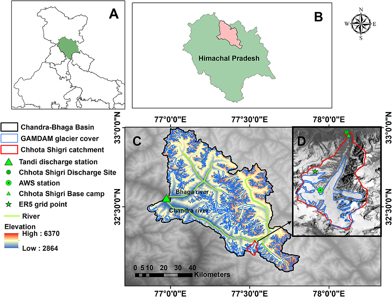
Figure 1. Location map of Chandra-Bhaga Basin (A–C), Basin boundary (black) with Tandi discharge site (green), river (green), and GAMDAM glacier cover (blue). Inset is the map of Chhota Shigri Catchment (D) with the catchment outline (red), Chhota Shigri Glacier (blue), and location of AWS station, discharge site, Chhota Shigri base camp, and ERA5 grid point (green symbols).
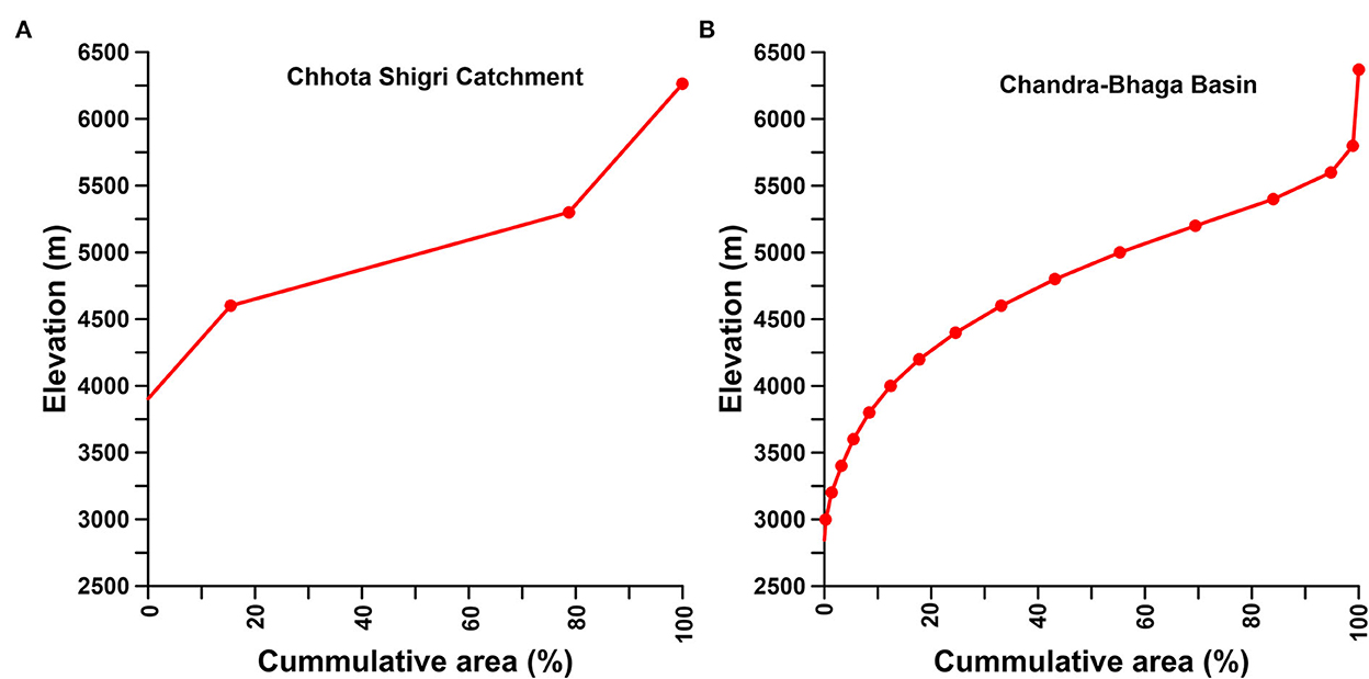
Figure 2. Hypsometry curve for Chhota Shigri Catchment (A) and Chandra-Bhaga Basin (B) showing the area distribution over the different elevations. Points represent the maximum elevations for each zone and cumulative percentage area.
The climate of the Chandra-Bhaga Basin is governed by two weather systems: Indian Summer Monsoon (ISM) and Western Disturbances (WDs; Dimri et al., 2015, 2016), however, 67% of the precipitation ( Mandal et al., 2020) come in the form of snow during winter months from WDs (Pratap et al., 2019; Singh et al., 2019; Mandal et al., 2020; Laha et al., 2021). The study region receives maximum precipitation in February and March from WDs (Mandal et al., 2020). Major discharge contribution in this basin is governed by the seasonal snow and glacier melt from major glaciers like Bara Shigri, Samudra Tapu, Sutri Dhaka, Batal, Chhota Shigri, and Hamtah, which are losing their mass over the last few decades (Singh et al., 2019; Mandal et al., 2020; Vishwakarma et al., 2022). In the Chhota Shigri Catchment, the discharge is dominated by snowmelt having around 69% contribution to the total discharge (Srivastava and Azam, 2022). The maximum discharge in the Chhota Shigri Catchment occurs in July-August corresponding to the maximum temperature (Mandal et al., 2020).
2.2. Datasets
2.2.1. DEM data and elevation zones
For snowmelt runoff modeling Cartosat Digital Elevation Model (DEM) having 30 m resolution was downloaded from the Bhuvan portal (https://bhuvan-app3.nrsc.gov.in) and extracted separately for both, the catchment and basin. The Chhota Shigri Catchment was divided into three 700 m interval elevation zones and the Chandra-Bhaga Basin was divided into sixteen 200 m interval elevation zones and their mean elevation and zone area were extracted using the digital elevation model (Table 1, Figure 2). The Chandra-Bhaga Basin was divided into the maximum possible number of elevation zones in SRM (WinSRM) but we kept a higher elevation difference in Chhota Shigri Catchment because the zonal areas were too small with the same elevation difference as Chandra-Bhaga Basin.
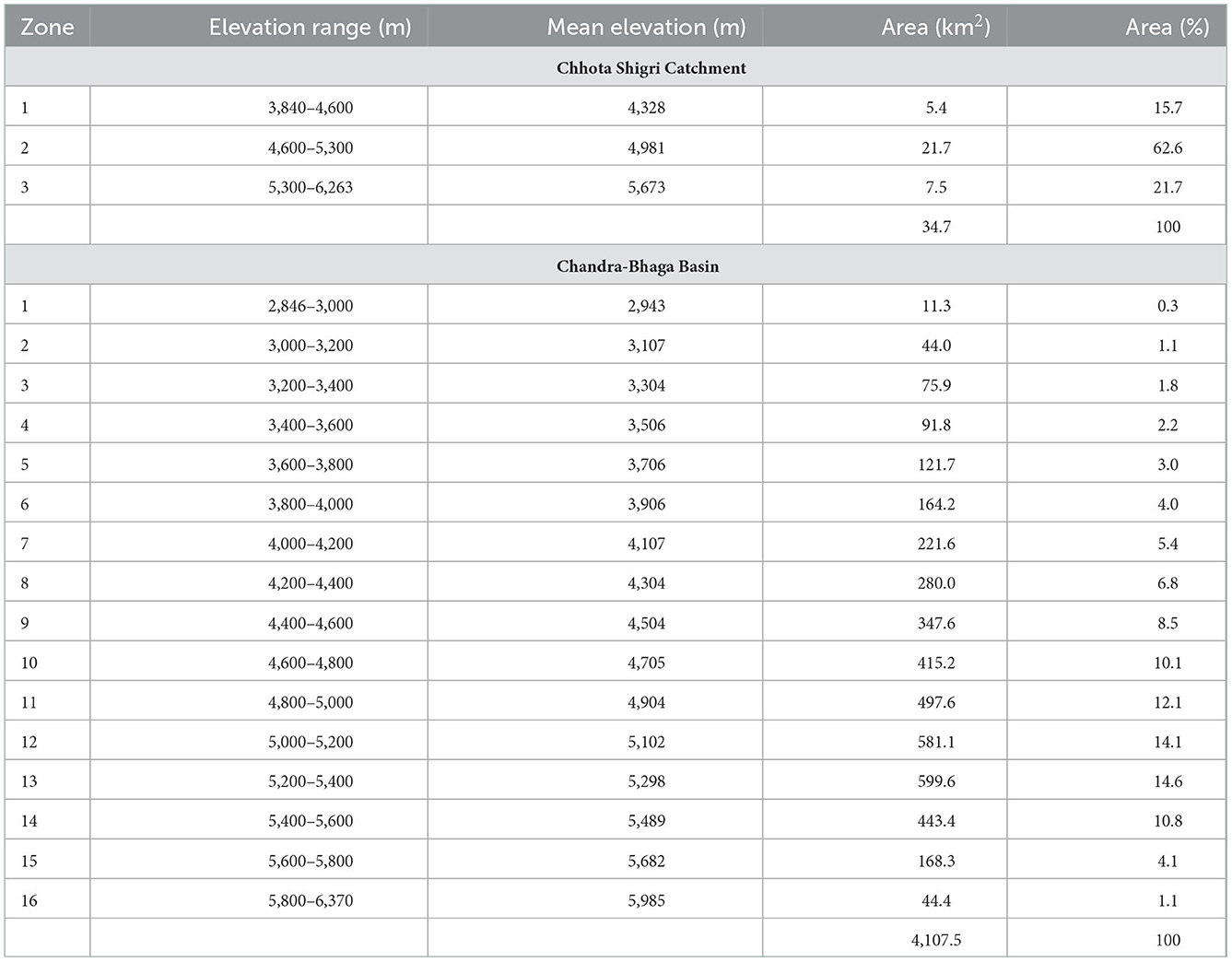
Table 1. Characteristics of different zones used in SRM for Chhota Shigri Catchment and Chandra-Bhaga Basin.
2.2.2. Meteorological data, discharge data, and bias correction
Reanalysis product ERA5 precipitation and temperature data at resolution 0.25° × 0.25° were downloaded (https://cds.climate.copernicus.eu) at the nearest ERA5 grid point to the automatic weather station (AWS) at 4,863 m a.s.l. in the Chhota Shigri Catchment (Figure 1D). ERA5 reanalysis data is available since 1950. For this study, the ERA5 temperature and precipitation data were bias-corrected using the field observations from the Chhota Shigri Catchment. The in-situ precipitation data was available from the Chhota Shigri base camp (3,850 m a.s.l.) over 2012–2020 from an automatic precipitation gauge (Geonor T-200B) and the temperature data was available from the AWS (Campbell CR1000 data logger; details can be found in Mandal et al., 2020; 4,863 m a.s.l.) in the Chhota Shigri Catchment over 2009–2019 (Azam et al., 2016; Mandal et al., 2020; Figure 1D). For the bias correction of temperature data, a linear regression equation was developed between the daily raw ERA5 temperature and the observed temperature, whereas monthly scale factors were used to bias correct the raw ERA5 precipitation series. The ERA5 bias-corrected data was used for snowmelt runoff modeling in the Chhota Shigri Catchment as well as Chandra-Bhaga Basin.
The ERA5 bias-corrected mean annual temperature at the nearest ERA5 grid point was −5.5°C over 2003–2018 with the maximum mean monthly and minimum mean monthly temperature of 4.1°C in July and −14.9°C in January. The mean monthly temperature for summer (May-September) was 1.2°C and for winter (January-April and October-December) it was −10.3°C (Figure 3). The ERA5 bias-corrected mean annual precipitation was 819.9 mm over 2003–2018 with maximum monthly precipitation of 129.7 mm in March and minimum monthly precipitation of 18 mm in November (Figure 3). The mean precipitation for summer and winter was 263.1 and 556.8 mm, respectively. The higher mean precipitation in winter shows that the major portion of the precipitation occurs in winter as suggested by previous studies (Azam et al., 2014; Mandal et al., 2020).
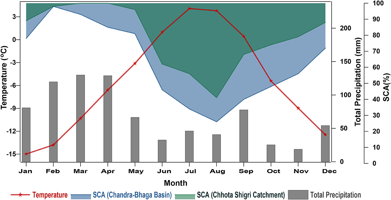
Figure 3. Monthly variation of model variables ERA5 bias-corrected (temperature and precipitation) and SCA for Chhota Shigri Catchment and Chandra-Bhaga Basin over 2003–2018.
The observed daily discharge data from Chhota Shigri Catchment at a gauging site (~3,840 m a.s.l.), ~2 km downstream of the Chhota Shigri glacier terminus, is available for the summer months over 2010–2015 (Azam et al., 2019). The measurement of discharge was done using the velocity-area method. A graduated staff gauge for monitoring the water level, dipsticks for measuring the cross-sectional area, and a current meter for the measurement of velocity were used (Mandal et al., 2020). The daily discharge measurements for the Chandra-Bhaga Basin are available over 2004–2006 at a gauging site located at Tandi village. This gauging site is maintained by the central water commission (CWC). For the measurement of discharge by CWC at this gauging site, the velocity-area method was used with a current meter for velocity, a rod and bamboo for depth measurement (http://cwc.gov.in/mco/discharge-observation).
2.2.3. Snow cover data
Snow cover data for the study area was available from an enhanced snow cover and glacier combined product MOYDGL06* at the 8-day interval for the period 2002–2018. This product is generated by reducing the overestimation caused by MODIS sensors and underestimation caused by cloud cover in MODIS snow cover products MOD10A2.006 (Terra) and MYD10A2.006 (Aqua; Muhammad and Thapa, 2020). This product is freely available in tiff format and WGS1984 projection (https://doi.pangaea.de/10.1594/PANGAEA.901821). For this study, a total of 736 images were used between 2003 and 2018. The SCA for each elevation zone of the Chhota Shigri Catchment and Chandra-Bhaga Basin was extracted for each 8-day interval and linearly interpolated to get the daily values.
In the Chhota Shigri Catchment, SCA was least in August (41% of the catchment area) and started increasing from September, achieved maximum SCA in March-April (100% of the catchment area), and then started decreasing in May (Figures 3, 4A). Whereas, in the Chandra-Bhaga Basin the SCA started increasing in September and decreased from March. Chandra-Bhaga Basin showed the maximum SCA in February (99% of the basin area) and the minimum SCA in August (26% of the basin area; Figures 3, 4B). The mean summer and winter SCA were 65% and 90%, respectively in the Chhota Shigri Catchment whereas for the Chandra-Bhaga Basin it was 45% and 76% of the total basin area, respectively.
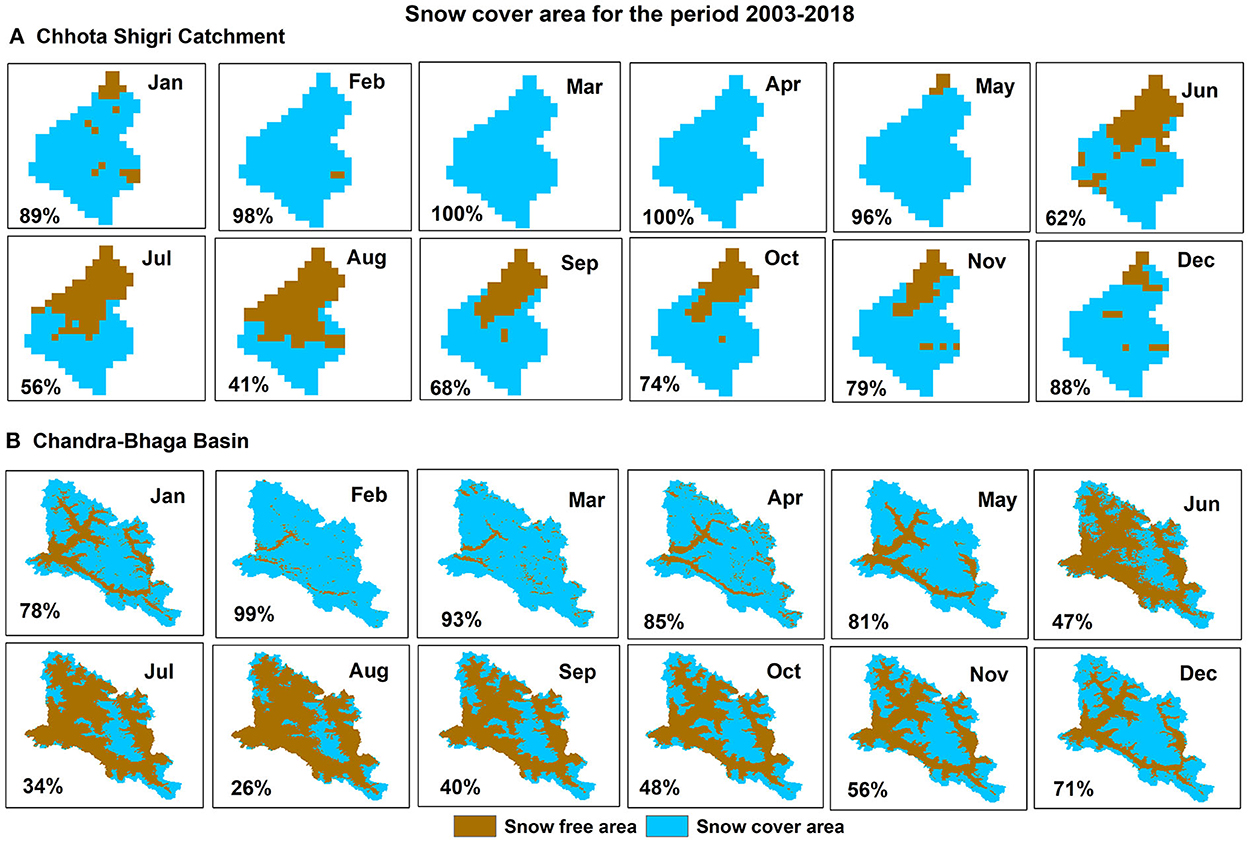
Figure 4. Mean monthly variation of SCA for Chhota Shigri Catchment (A) and Chandra-Bhaga Basin (B) over 2003–2018. Maps of both the areas are not on the same scale.
3. Methodology
3.1. Snowmelt runoff model
SRM (WinSRM version 1.12) is based on the degree-day approach and runs for a maximum of 366 days in one simulation. This model can be applied in two ways basin-wide and zone-wise applications. For reconstructing the discharge in the Chhota Shigri Catchment and Chandra-Bhaga Basin, we ran the model zone-wise to compute the catchment-wide or basin-wide discharge. The simulated discharge is a combination of snowmelt runoff and rainfall runoff superimposed on recession flow to transform all the components into daily discharge (Martinec et al., 2007). This model follows Equation 1 for the daily discharge computation from each zone:
Where Q is the daily discharge in m3/s, CS and CR are the runoff coefficients for snow and rain, respectively, a is the degree-day factor (cm °C−1 d−1), Tn+△Tn are the degree days (°C d−1) after extrapolation for each zone mean elevation, S is the ratio of snow-covered area to the zone area, P is precipitation contributing to runoff (cm), A is the zone area (km2), k is the recession coefficient (input as “x” and “y” in the model) and n shows the sequence of days.
The critical temperature (Tcrit) is used to decide the precipitation phase as snow or rain. If the precipitation is determined as snow, its delayed effect is considered in two ways: (1) snowfall over the snow-covered area is assumed to become part of the snowpack and its contribution is determined by the snow depletion curve (Martinec et al., 2007) and (2) snowfall occurring over snow-free areas contributes to the discharge immediately, depending on the available degree days. When the precipitation is determined as rain its contribution to the discharge depends on the snowpack characteristics. In winter, the snowpack is dry and thick so the rain falling over the SCA is retained by the snowpack and the rain contribution to the total runoff is limited to the only snow-free area. Later in summer, the snow becomes ripe, and the rain is allowed to contribute to the runoff from the entire zone area. The rainfall-induced melting and base flow (sub-surface fluxes) are ignored in SRM (Martinec et al., 2007). Further, the glacier ice melt contribution is also ignored (Tahir et al., 2011).
3.2. Model parameters
In SRM, a total of nine different parameters are used. These parameters are runoff coefficient for snow and rain (CS and CR), degree-day factor (a), temperature lapse rate (LR), critical temperature (Tcrit), time lag, recession coefficients (x and y), and rainfall contributing area (RCA). In rough terrain like the Himalaya, the measurement of these parameters is very difficult because of the remote access and adverse climate conditions. But the Chhota Shigri Catchment is one of the glacier catchments which is having the longest series of observed meteorological data and discharge measurements (Azam, 2021), hence among the nine parameters three parameters (LRs, “x” and “y”) were calculated and constrained using the field measurements in the Chhota Shigri Catchment, whereas the other model parameters were calibrated for the Chhota Shigri Catchment.
CS and CR represent the losses between the available water (snowmelt + rainfall) and the runoff volume from the catchment or basin, it depends on the surface conditions in the catchment or basin. The default values of CS and CR in the model were adopted initially for the Chhota Shigri Catchment as 0.7 and 0.6 for CS and CR, respectively (Martinec et al., 2007). “a” is converting the positive temperatures on a particular day into the melt depth. For the Chhota Shigri Catchment, the initial “a” was considered as 5.28 mm °C−1 d−1 (Azam et al., 2014). The daily temperature LRs for the Chhota Shigri Catchment were available between the two temperature measurement stations at 3,850 m a.s.l. (base camp) and 4,863 m a.s.l. (AWS station; Mandal et al., 2022; Srivastava et al., 2022). The mean LR was 0.63 °C (100 m)−1 and it was 0.71°C (100 m)−1 for summer (May-September) and 0.57 °C (100 m)−1 for winter (October–April). For precipitation extrapolation, we adopted a precipitation gradient (PG) of 0.20 m/km constrained through a mass balance model calibration on the Chhota Shigri Glacier (Azam et al., 2014). Tcrit is the threshold temperature that determines the precipitation phase. The time lag is the time interval between the start of increasing temperature and the corresponding increase in discharge. For both, the catchment and basin, we have adopted the time lag range from 6 to 18 h varying with the elevation zones from previous studies (Martinec et al., 2007; Tahir et al., 2011; Panday et al., 2014). The time lag tends to increase with elevation because at higher elevations, the mean temperature is less and the travel time for the melted water to the discharge point is more as compared to the lower zones, which results in the delayed discharge from the higher elevations. k deals with the proportion of the daily discharge which appears immediately in the runoff. In the SRM, this coefficient is used in the form of “x” and “y,” which is usually determined by the historical discharge series. Based on the relation between k, “x,” “y,” and discharge i.e., and the values of “x” and “y” can be determined (Martinec et al., 2007). In our study, we have calculated the value of “x” and “y” from the available discharge series for the Chhota Shigri Catchment and Chandra-Bhaga Basin. The RCA was taken as 1 for summer and 0 for winter depending on the melting season for both catchment and basin. RCA 1 represents that the rain from the total zone area is contributing to the runoff and 0 shows that rain only from the snow-free area is contributing to the runoff.
3.3. Model variables
Precipitation, temperature, and SCA are the three most important input variables in SRM which are required to simulate the daily discharge (Martinec et al., 2007). We extrapolated the bias-corrected temperature and precipitation data from the ERA5 grid point for the mean altitude of each elevation zone using the daily LR and PG, respectively, available from previous studies in the Chhota Shigri Catchment (Azam et al., 2019; Srivastava et al., 2022). The extrapolated daily temperature and precipitation values were fed in the model, separately for each zone in both Chhota Shigri Catchment and Chandra-Bhaga Basin. The model also needs daily SCA fractions as an input which is the ratio of zonal SCA to the total zonal area. For each zone, these values were calculated at a daily timestep as discussed in Section 2.2.3.
3.4. Model calibration and validation
The model for the Chhota Shigri Catchment was calibrated with the observed discharge values over 2010–2013 (Figure 5A). The parameters Tcrit, “a,” CS, CR, x, and y were calibrated over 2010–2013 while LR, time lag, and RCA were kept constant. The calibrated parameters were kept within a permissible range corresponding to the previous studies on SRM to avoid the overfitting of the model. The calibration was done by considering different performance criteria i.e., coefficient of determination (R2), RMSE, and NSE (Nash-Sutcliff efficiency) that is determined using the equation:
Here, n, Oi, are the number of observations, observed discharge, simulated discharge, mean observed discharge and mean simulated discharge, respectively (Nash and Sutcliffe, 1970). NSE lies between 1 and −∞ where 1 corresponds to the perfect match and R2 lies between 0 and 1. The calibrated parameters are shown in Table 2.
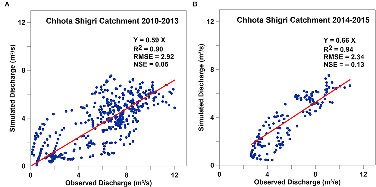
Figure 5. Scatter plots for calibration on Chhota Shigri Catchment over 2010–2013 (A) and validation on Chhota Shigri Catchment over 2014–2015 (B). Plots are showing the relations between observed and simulated discharges.
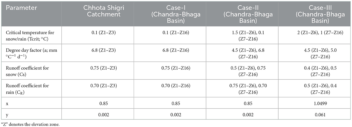
Table 2. List of calibrated parameters and their calibrated values for the Chhota Shigri Catchment over 2010–2013 and Chandra-Bhaga Basin over 2004–2006.
3.5. Sensitivity and uncertainty estimation
To understand the sensitivity of simulated discharge to different model parameters, sensitivity analysis was performed for eight model parameters including k (x and y), CS, CR, “a,” Tcrit, LR, and time lag. The sensitivity analysis was performed separately for both the Chhota Shigri Catchment and Chandra-Bhaga Basin over 2003–2018. For sensitivity analysis, each parameter was increased and decreased one by one by 10, 20, and 30% while keeping all other parameters constant, and the sensitivities were estimated using simulated mean daily discharge (Oerlemans et al., 1998) as following:
Here, S is the sensitivity of each parameter, QH and QL is the mean daily discharge values at the highest (+10, +20, and +30%) and lowest (−10, −20, and −30%) values of parameters.
For the uncertainty estimation in the simulated discharge, each model parameter among x, y, CS, CR, “a,” and Tcrit were changed one by one, within a 10% range of its calibrated value (Heynen et al., 2013; Ragettli et al., 2013). The parameters which were not calibrated kept the same i.e., LR, time lag, and RCA, using the field observations from Chhota Shigri Catchment, are not changed in this process. The uncertainty estimation was done for both the study region Chhota Shigri Catchment and Chandra-Bhaga Basin separately. The overall mean uncertainty in the simulated daily discharge was estimated using the error propagation law as following:
Here, U is the overall uncertainty, n is the number of parameters, and Q+10% and Q−10% are the mean daily simulated discharge when the parameters increased and decreased by 10%.
4. Results and discussions
4.1. Calibration and validation
The calibrated daily discharge over 2010–2013 showed a good agreement with the observed data (R2 = 0.90, RMSE = 2.92 and NSE = 0.05; Figure 5A). However, the mean calibrated discharge showed an underestimation of 41% (Figures 5A, 7A). As already highlighted, we kept all the model parameters within plausible ranges based on previous studies to avoid overfitting of the SRM. The 41% underestimation is most probably due to the lack of baseflow and glacier melt contribution in the SRM (details in Section 4.7). After the calibration, the SRM output for the Chhota Shigri Catchment was validated with the observed discharge over 2014–2015. In validation the mean simulated discharge showed a good agreement with the observed discharge (R2 = 0.94, RMSE = 2.34, and NSE = −0.13; Figure 5B) but with an underestimation of 34% (Figures 5B, 7A). After the validation, the same calibrated model was used to simulate the daily discharge for the Chhota Shigri Catchment over 2003–2018.
The observed daily discharge was also available for the Chandra-Bhaga Basin over 2004–2006. To check the transferability of catchment-scale calibrated model parameters to basin-scale discharge simulation, the discharge for Chandra-Bhaga Basin was simulated over 2004–2006 for two different case scenarios. Case-I: the calibrated parameters on Chhota Shigri Catchment were applied on all the zones in Chandra-Bhaga Basin and Case-II: the calibrated parameters were applied on zones having elevation above 3,900 m a.s.l., as the Chhota Shigri Catchment is having a minimum elevation of ~3,900 m a.s.l. and altered parameters (based on previous SRM studies) were applied for zones below 3,900 m a.s.l.
In Case-II, for the zones below 3,900 m a.s.l., the parameters were altered based on previous studies (Tahir et al., 2011; Panday et al., 2014). We adopted a lower value of “a” (4.5 mm °C−1 d−1) for the lower zones because “a” is expected to decrease with a decrease in elevation, due to the high direct solar radiation at higher altitudes (Hock, 2003; Zhang et al., 2006; Tahir et al., 2011; Panday et al., 2014). Tcrit for rain/snow separation was taken as 1.5°C for lower zones, like the previous studies in the western Himalaya (Singh and Jain, 2003; Aggarwal et al., 2014; Kiba et al., 2021). The values of CS and CR were also varied with the zone elevation, for the higher altitudes, the values for CS are higher and the values for CR are less as compared to the lower zones (Tahir et al., 2011; Panday et al., 2014). In the Chandra-Bhaga Basin for the lower elevations (below 3,900 m a.s.l.), the values for these coefficients were altered as 0.5 and 0.75 for CS and CR, respectively. The values of x, y, RCA, time lag, and LR were kept the same as the Chhota Shigri Catchment for all the zones (Table 2).
With the above-mentioned values of all the parameters for Case-I and Case-II (Table 2), the daily discharge for Chandra-Bhaga Basin was simulated over 2004–2006. The daily simulated discharge in both the cases showed a good agreement with the observed discharge over 2004–2006 (Figures 6A, B) but an overestimation of 83% in Case-I and an overestimation of 74% in Case-II. Despite the underestimation in simulated discharge at Chhota Shigri Catchment, large discharge overestimation in the Chandra-Bhaga Basin showed that the catchment-scale calibrated parameters are not transferable for basin-scale discharge simulation. This overestimation is further discussed in Section 4.7.
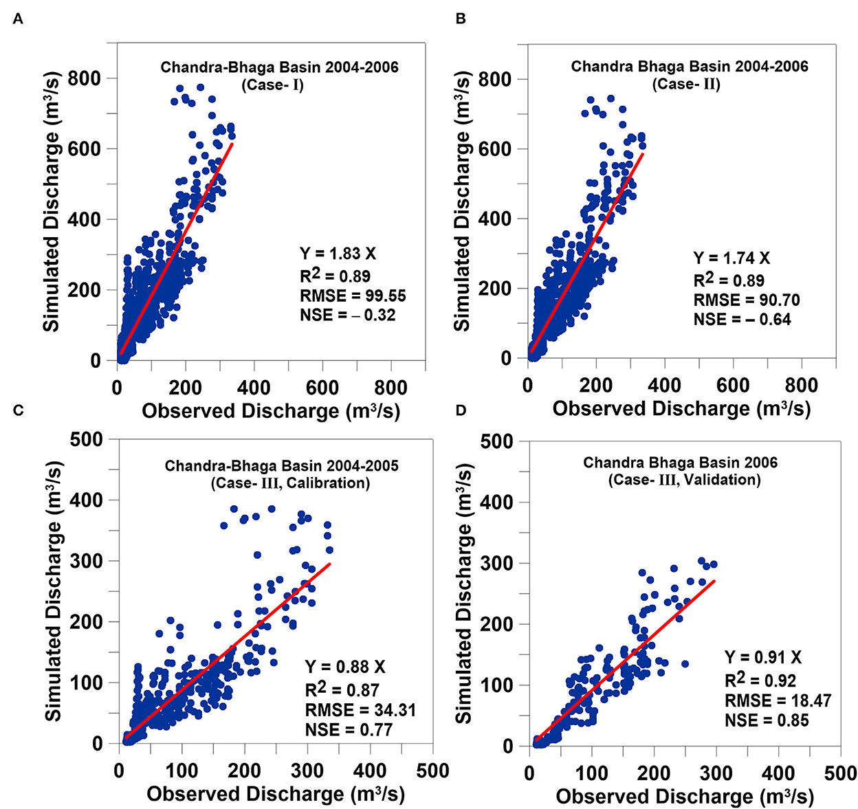
Figure 6. Scatter plots between the observed and simulated discharge for Chandra-Bhaga Basin in all three case scenarios (A) Chandra-Bhaga Basin 2004–2006 (Case-I), (B) Chandra-Bhaga Basin 2004–2006 (Case-II), (C) Chandra-Bhaga Basin 2004–2005 (Case-III, calibration), and (D) Chandra-Bhaga Basin 2006 (Case-III, validation).
Apart from these two case scenarios (Case-I and Case-II), where the Chandra-Bhaga simulated discharge is largely overestimated, we performed an independent model calibration for the Chandra-Bhaga Basin using the discharge data from Tandi village (Case-III; Table 2), ignoring the calibrated parameters on Chhota Shigri Catchment. The calibrated daily discharge over 2004–2005 showed a good agreement with the observed data with R2 = 0.87, RMSE = 34.31, and NSE = 0.77 (Figure 6C). After the calibration, the same model was validated with the observed data for 2006 that showed a good agreement with R2 = 0.92, RMSE = 18.47, and NSE = 0.85 (Figure 6D). The calibrated and validated modeled discharge in Chandra-Bhaga Basin showed an underestimation of 12 and 9%, respectively unlike the overestimation shown in Case-I and Case-II for the same basin. The daily discharge for the Chandra-Bhaga Basin was simulated with these calibrated parameters over 2003–2018.
4.2. Reconstructed daily discharge and its pattern
The discharge from Chhota Shigri Catchment and Chandra-Bhaga Basin was reconstructed for 2003–2018 at a daily time step (Figure 7). The mean of daily discharges over 2003–2018 for the Chhota Shigri Catchment was 1.2 ± 0.2 m3/s (Figure 7A). In the Chhota Shigri Catchment, the simulated daily discharge starts increasing in April and reaches the maximum in July. The highest peak in daily discharge was observed on 11th July 2005 of 7.9 ± 1.4 m3/s. The mean of daily discharges in the Chandra-Bhaga Basin was 55.9 ± 12.1 m3/s over 2003–2018 (Figure 7B). The daily discharge starts increasing in March and reaches its peak in July. The highest daily discharge was observed on 16th July 2011 of 386.7 ± 21.2 m3/s. The observed daily discharge values for the Chhota Shigri Catchment over 2010–2015 and for Chandra-Bhaga Basin over 2004–2006 are also shown in Figure 7. The comparison showed that the simulated discharge in both; the catchment and basin was underestimated (discussed in Section 4.1).
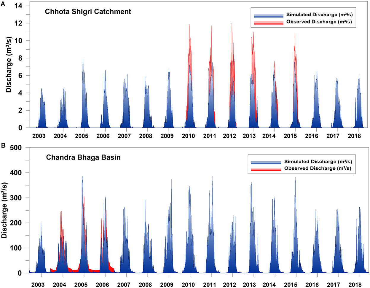
Figure 7. Simulated discharge of Chhota Shigri Catchment (A) and Chandra-Bhaga Basin (B) over 2003–2018 (blue color). The observed discharge for Chhota Shigri Catchment (A) and Chandra-Bhaga Basin (B) in red color over 2010–2015 and 2004–2006, respectively.
4.3. Seasonal and annual discharge patterns
To understand the seasonal and annual patterns, the seasonal and annual discharge was computed using daily simulated discharge for Chhota Shigri Catchment and Chandra-Bhaga Basin over 2003–2018. Summer discharge has been considered from May to September and winter discharge has been considered from October to December and January to April in the same year. The mean summer discharge and winter discharge were found as 2.7 ± 0.5 and 0.1 ± 0.05 m3/s for Chhota Shigri Catchment, Similarly, for Chandra-Bhaga Basin it was 123.9 ± 22.3 and 6.7 ± 3.3 m3/s, respectively. The simulated discharge ranged from 0.02 ± 0.01 to 0.2 ± 0.04 m3/s and 2.6 ± 1.2 to 13.3 ± 4.7 m3/s in winter and 1.9 ± 0.3 to 3.4 ± 0.6 m3/s and 77.6 ± 13.7 to 164.5 ± 28.3 m3/s in summer for Chhota Shigri Catchment and Chandra-Bhaga Basin, respectively. The annual discharge is the mean discharge in both seasons over the same year. The mean annual discharge for the Chhota Shigri Catchment was found as 1.2 ± 0.2 m3/s over 2003–2018 with a minimum annual discharge of 0.8 ± 0.1 m3/s in 2004 and a maximum of 1.5 ± 0.3 m3/s in 2011 (Figure 8B). The mean annual discharge for the Chandra-Bhaga Basin was found as 55.9 ± 12.1 m3/s over 2003–2018 with a minimum annual discharge of 39.9 ± 9.1 m3/s in 2003 and a maximum annual discharge of 75.1 ± 13.2 m3/s in 2010 (Figure 8C). The mean summer discharge dominates the mean winter discharge over 2003–2018 in the Chhota Shigri Catchment as well as in the Chandra-Bhaga Basin. Similar results were also suggested for the Chhota Shigri Catchment and Chandra Basin in the western Himalaya (Singh et al., 2021; Gaddam et al., 2022; Srivastava and Azam, 2022).
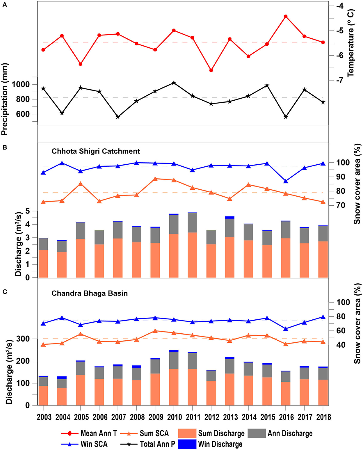
Figure 8. Seasonal (summer in orange and winter in blue) and annual (gray) discharge patterns over 2003–2018 with total precipitation (black) and mean temperature (red) patterns for Chhota Shigri Catchment (B) and Chandra-Bhaga Basin (C). The summer season is from May to September and the winter season is from October to December and January to April. Total precipitation and mean temperature patterns plotted here represent the data from the ERA5 grid point location (A). Dashed lines are showing the average values over 2003–2018 of temperature (red), precipitation (black), winter SCA (blue), and summer SCA (orange).
The year 2016 has the maximum temperature and minimum precipitation (Figure 8A). It is noteworthy that the 2016 year was the warmest over a century (Wuebbles et al., 2017). This year, though the winter SCA was relatively less, the Chhota Shigri catchment showed more than the average discharge because of excessive snowmelt runoff production, mainly supported by quasi average summer SCA (Figure 8B). Conversely, in the Chandra-Bhaga Basin, the modeled discharge was less than average because of the lowest precipitation (Rain + Snow), and lowest winter as well as summer SCA (Figure 8C). Similarly, in 2011 the Chhota Shigri Catchment showed the maximum discharge having average precipitation and associated with the higher snowmelt due to higher temperature and higher summer SCA (Figure 8B). While the Chandra-Bhaga Basin showed the maximum discharge in 2010 due to the maximum precipitation and higher summer SCA (Figure 8C).
Further, to understand the influence of variables on discharge, the interrelationships between the discharge (annual, summer, and winter), SCA (annual, summer, and winter), and temperature and precipitation (annual, summer, and winter) were explored with the help of the correlation matrix developed separately for both the study regions (Figure 9). In both the study regions, the annual discharge is highly correlated with the summer discharge as the maximum melting occurs in summer (Figure 9). The annual discharge in the Chhota Shigri Catchment is more correlated with summer temperature (r = 0.51) and summer SCA (r = 0.47) and has a very weak correlation with the annual precipitation (Figure 9A). These relations are expected because the higher altitude of the catchment provides more snowfall than rainfall hence catchment discharge is mainly dominated by snowmelt. Similarly, the summer discharge also showed the same relationship with the summer temperature and summer SCA (Figure 9A). Due to very low temperatures, winter discharge was negligible (4% of summer discharge) hence relationships were insignificant.
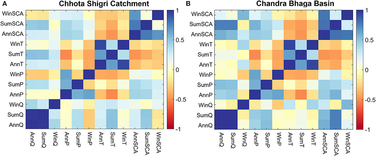
Figure 9. Correlation matrix for Chhota Shigri Catchment (A) and Chanda-Bhaga Basin (B). The values from −1 to 1 denote the correlation coefficients and the color range denotes the intensity of the correlation (one denotes the completely positive correlation, dark blue, and −1 denotes the completely negative correlation, dark brown). Ann, Sum, and Win are annual, summer, and winter season and Q, P, T, and SCA are discharge, precipitation, temperature, and SCA, respectively.
In the Chandra-Bhaga Basin, the annual discharge showed a strong correlation with the summer SCA (r = 0.74) followed by summer precipitation (r = 0.53; Figure 9B) as the basin, has lower altitudes (up to 2,804 m a.s.l.), receives a significant contribution of rainfall that directly contributes to discharge. The same relation was also shown by the summer discharge with summer SCA and summer precipitation (Figure 9B). Though the winter discharge was only 6% it was fairly correlated with the winter SCA (r = 0.56) and winter temperature (r = 0.41; Figure 9) because sometimes at lower altitudes positive temperatures may occur in March and April which generates some snowmelt. In all, the discharge in Chhota Shigri Catchment is equally driven by both summer temperature and summer SCA while in the Chandra-Bhaga Basin summer SCA and summer precipitation exert a strong control on the discharge.
4.4. Contribution of different components to total discharge
The modeled discharge from SRM includes the contribution from rainfall and snowmelt. The snowmelt is considered in two ways: melt from “New snow” and “Initial snow.” “New snow” melt is the sum of melts from the snow melt from nth day snowfall and remained snow on the previous days from the non-snow cover area in the catchment. “Initial snow” melt is the melt contribution coming from the depletion of snow cover. The percentage contribution of different components in discharge for Chhota Shigri Catchment and Chandra-Bhaga Basin is shown in Figure 10.
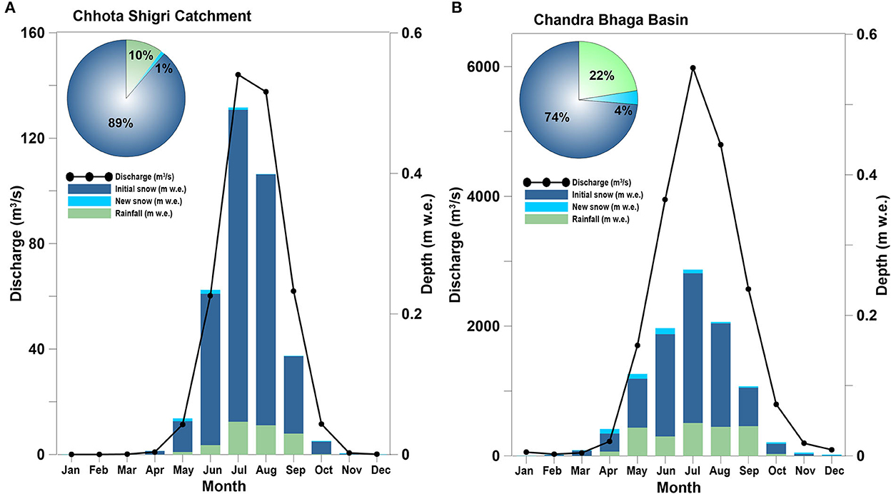
Figure 10. Monthly hydrograph of total discharge (black line) and depth of different components contributing to the total discharge: initial snow (blue), new snow (sky blue), and rainfall (light green) over 2003–2018 for Chhota Shigri Catchment (A) and Chandra-Bhaga Basin (B). The pie chart is showing the percentage contribution of each component.
The percentage contribution of snowmelt as initial snow from SCA to total discharge was highest with 89 and 74% in Chhota Shigri Catchment and Chandra-Bhaga Basin, respectively. The contribution of monthly snowmelt from the SCA was maximum over July in both the study regions in agreement with the maximum monthly mean temperatures (Figure 3). As expected, the contribution of total snow melt (initial snow + new snow) to total discharge was significantly more in the Chhota Shigri Catchment (90%) compared to the Chandra-Bhaga Basin (78%; Figure 10). Whereas, the contribution of new snow was higher in Chandra-Bhaga Basin (4%) as compared to the Chhota Shigri Catchment (1%). The higher melt contribution of new snow in the Chandra-Bhaga Basin was due to the higher temperatures at the lower zones (below 3,900 m a.s.l.) than Chhota Shigri Catchment, which promotes the melting of new snow. As expected, the rainfall contribution to total discharge was higher (22%) in the Chandra-Bhaga Basin than in the Chhota Shigri Catchment (10%) due to the lower elevation zones (below 3,900 m a.s.l.) that favor more rainfall due to higher temperatures.
The monthly depth (new snowmelt + initial snowmelt + rainfall) was maximum in July as 0.49 ± 0.03 and 0.27 ± 0.02 m w.e. for Chhota Shigri Catchment and Chandra-Bhaga Basin, respectively (Figures 10A, B). The total annual depth (1.34 ± 0.01 m w.e.) in Chhota Shigri Catchment was more than the Chandra-Bhaga Basin (0.93 ± 0.05 m w.e.) because the higher Tcrit (1°C at above 3,900 m a.s.l. and 2°C at below 3,900 m a.s.l.) in the Chandra-Bhaga Basin compared to Tcrit (0.1°C) in the Chhota Shigri Catchment results in a relatively higher amount of snow available for melt from snowfall (Section 4.1). Snow takes relatively more time to contribute to the discharge and sometimes may not produce melt due to limited degree days and become part of storage that is nullified at the end of each calendar year, a limitation of the SRM discussed in Section 4.7. Due to the lower Tcrit (0.1°C) a larger portion of precipitation is considered as rainfall in Chhota Shigri Catchment which directly contributes to the discharge and further results in higher depth than Chandra-Bhaga Basin.
4.5. Decadal discharge patterns
Studies suggest that volumetric and seasonal changes are occurring in the HK river runoffs due to climate change (Lutz et al., 2014; Azam et al., 2021). Though, our simulation period is short (2003–2018), we analyzed the decadal variations in discharge by comparing two time periods of equal length as 2003–2010 and 2011–2018. A higher discharge was found over 2011–2018 period than 2003–2010 period in both Chhota Shigri Catchment and Chandra-Bhaga Basin. The mean monthly discharge in the Chhota Shigri Catchment increased by 8% from 1.1 ± 0.2 to 1.2 ± 0.3 m3/s over 2011–2018 as compared to 2003–2010. Similarly in the Chandra-Bhaga Basin, the mean monthly discharge increased by 2% from 54.9 ± 11.2 to 56.2 ± 13.9 m3/s over 2011–2018 as compared to 2003–2010. In both the study regions, the maximum monthly discharge occurred in July (Figure 11). The maximum monthly discharge increased by 11% from 4.4 ± 0.7 to 4.9 ± 0.7 m3/s for the Chhota Shigri Catchment and by 9% from 184.1 ± 25.9 to 201.8 ± 24.8 m3/s for the Chandra-Bhaga Basin in 2011–2018 as compared to 2003–2010 (Figures 11A, B).
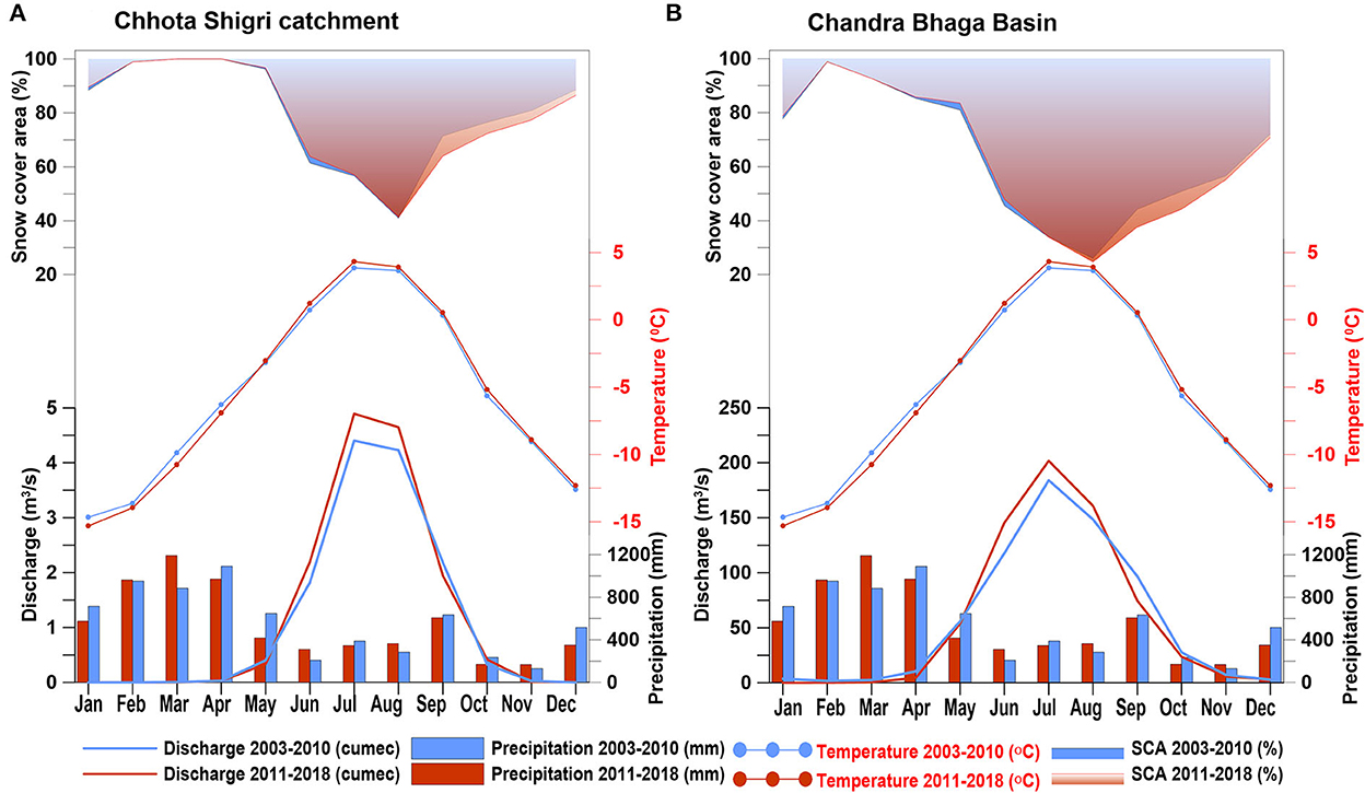
Figure 11. Decadal comparison of discharge with precipitation, temperature, and snow cover area over the two time periods 2003–2010 (blue color) and 2011–2018 (red color) for Chhota Shigri Catchment (A) and Chandra-Bhaga Basin (B).
In the Chhota Shigri Catchment, the mean monthly discharge over June-August increased by 11% from 4.3 ± 0.64 m3/s in the 2003–2010 to 4.8 ± 0.76 m3/s in 2011–2018 (Figure 11A). This increased discharge was due to the increased temperature in 2011–2018 (3.3°C) as compared to 2003–2010 (2.7°C) over June-August (Figure 11), having almost the same SCA in both periods (53 and 54%). Conversely, the discharge decreased in September over 2011–2018 as compared to 2003–2010 due to the lower SCA (64% as compared to 71%), even having a higher temperature by 0.2°C in 2011–2018 (Figure 11A). In the Chandra-Bhaga Basin, the mean monthly discharge also increased in summer by 11% from 126.5 ± 20.6 m3/s over 2003–2010 to 140.4 ± 30.4 m3/s over 2011–2018, except in September (Figure 11B). This increment in summer discharge resulted due to the increased precipitation from 882 mm in 2003–2010 to 1,023 mm in 2011–2018 (over June-August) and increased SCA (over May-June) from 63% in 2003–2010 to 66% in 2011–2018 (Figure 11B). Similarly, in September the decreased precipitation by 27 mm and decreased SCA (37% as compared to 44%) resulted in lower discharge in the basin (Figure 11B). Though the summer discharge increased, the winter discharge decreased in both the study regions over 2011–2018 period. In the Chhota Shigri Catchment the variations were negligible (< 1%) whereas in the Chandra-Bhaga Basin the winter discharge showed a significant decrease of 32% from 7.9 ± 5.2 m3/s over 2003–2010 to 5.3 ± 3.4 m3/s over 2011–2018 due to the decreased temperature over January-April by 0.6°C in 2011–2018 and decreased SCA (56% as compared to 60%) over October-December (Figure 11B). In line to Section 4.3, the decadal analysis also suggested a large control of summer temperature and summer SCA in the Chhota Shigri Catchment and summer SCA and summer precipitation in Chandra-Bhaga Basin, for discharge generation in summer, and winter temperature and winter SCA control on winter discharge in the Chandra-Bhaga Basin.
Further, the hydrograph is also slightly shifted in early summer ~10 days in the Chhota Shigri Catchment and 20 days in the Chandra-Bhaga Basin. The early onset of discharge or the seasonality shift was also observed in previous studies in the Indus Basin (Immerzeel et al., 2010; Tahir et al., 2011; Lutz et al., 2014; Hasson, 2016). In our study, we observed this change in seasonality occurred due to the higher temperatures and higher SCA in the early summer months (May and June) and also the early occurring precipitation peak in March over 2011–2018 as compared to April over 2003–2010 (Figure 11). Similar to our study Immerzeel et al. (2010) and Lutz et al. (2014) also highlighted the increased precipitation and shift in the snowmelt peak (due to high temperature) as the main cause of the seasonality shift in the Indus Basin.
4.6. Sensitivity analysis
In the Chhota Shigri Catchment, the simulated discharge was almost equally sensitive to “a” and CS with a sensitivity of 0.098 and 0.099 m3/s, respectively (Figure 12A, Table 3). Other parameters CR, and LRs showed mean sensitivities of −0.011 m3/s and 0.015 m3/s, respectively, whereas the model is less sensitive to “x” and Tcrit (Table 3). Parameters “y” and time lag showed no impact on simulated discharge in the Chhota Shigri Catchment. In the Chandra-Bhaga Basin, the simulated discharge was most sensitive to CS with a sensitivity of 5.2 m3/s followed by “a” with a sensitivity of 5.0 m3/s (Figure 12B, Table 3) whereas among the other parameters the model is more sensitive to CR, and LR as compared to “x” and Tcrit with “y” and time lag have no impact on simulated discharge, similar to the Chhota Shigri Catchment (Table 3). Other studies by Panday et al. (2014) and Siemens et al. (2021) also found that the parameters CS, CR, “x,” and “y” have substantial control over the simulated discharge. The analysis showed almost linear changes in the simulated discharge with variations in each sensitive parameter value except for parameter “x” (Figure 12). The simulated discharge varied significantly when the parameter value of “x” increased from 10 to 20% and become constant after this. Whereas, it showed no significant change in the discharge when the value of “x” was reduced. This varying pattern was due to the maximum limit of k as 0.99 in WinSRM (Section 3.2), which restricts the value of “x” and “y” according to the maximum value of k. We found a significant impact of LR on simulated discharge, which is also highlighted by Jain et al. (2010) and Panday et al. (2014). In our study, we used daily temperature LRs observed in the Chhota Shigri Catchment which is among the sensitive parameters in both the study regions. The adopted daily LR values enable the SRM to capture the seasonal variations in the discharge (Figure 8) which is not possible with constant LR values over a year. The daily LRs reduce the possibility of errors in the extrapolated temperature values which directly affects the snowmelt in the different seasons. The overall mean uncertainty in the simulated daily discharge was found as ± 0.2 and ± 12.1 m3/s for Chhota Shigri Catchment and Chandra-Bhaga Basin, respectively.
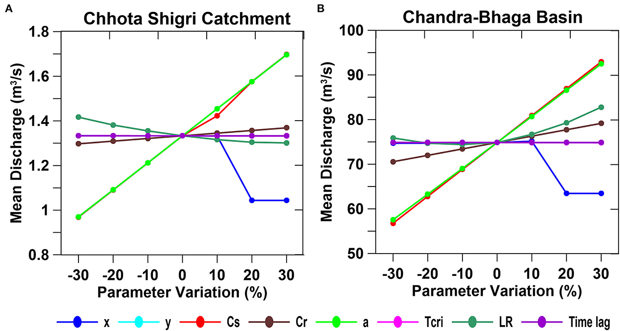
Figure 12. Sensitivity analysis results for Chhota Shigri Catchment (A) and Chandra-Bhaga Basin (B). The X-axis shows the percentage variation in the values of each parameter and the Y-axis shows the corresponding simulated mean daily discharge values.
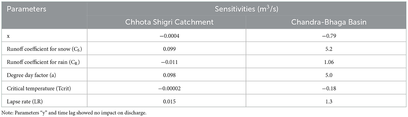
Table 3. List of model parameters and their sensitivities for the Chhota Shigri Catchment and Chandra Bhaga Basin (Case-III).
4.7. Model limitations and transferability of catchment-scale calibrated model parameters to basin scale
In Section 4.1, we introduced the model limitations and transferability of catchment-sale calibrated model parameters to basin-scale discharge simulation in the same basin. In this section, we investigated this in detail. The simulated daily discharge in the Chhota Shigri Catchment was underestimated (41 and 34%) over the calibration (2010–2013) and validation (2014–2015) periods, respectively (Figures 5A, B, 7A). The SRM does not involve the baseflow and glacier melt runoff contribution to the total discharge. Given that the Chhota Shigri Catchment is highly glacierized (47%), base flow contribution can be neglected (Srivastava and Azam, 2022). However, glacier melt contribution cannot be ignored, and probably this is the reason for the underestimation in simulated discharge as glacier provides significant runoff contribution through glacier melt (around 21% of the total runoff; Srivastava and Azam, 2022). In line, the simulated discharge in Case-III for the Chandra-Bhaga Basin was also underestimated (12% over 2004–2005 and 9% over 2006). The relatively less underestimation in the Chandra-Bhaga Basin is probably associated with the less glacierized area (25%) in the Chandra-Bhaga Basin as compared to the Chhota Shigri Catchment (47%). Another reason for this underestimation in SRM simulated discharge in both the catchment and basin scale could be the stored snow at higher altitudes (above zero-degree isotherm) which does not melt at the end of the year and cannot be added to the next successive year's simulation in the SRM scheme.
Conversely, when the calibrated model parameters from Chhota Shigri Catchment were applied to simulate the discharge from the Chandra-Bhaga Basin, the simulated discharge in Chandra-Bhaga Basin in Case-I and Case-II was overestimated (83 and 74%) by the SRM over 2004–2006 (Section 4.1; Figures 6A, B). The overestimation in simulated discharge could partially be due to the parameter values which may not be applicable for lower elevation zones (below 3,900 m a.s.l.) in Chandra-Bhaga Basin. The precipitation phase (snow vs. rain) patterns over Chhota Shigri Catchment and lower zones of Chandra-Bhaga Basin (below 3,900 m a.s.l.) are quite different as the Chhota Shigri Catchment receives frequent snowfall while the Chandra-Bhaga Basin is having relatively more rainfall frequency due to the inclusion of the lower altitudes in the basin. The values of Tcrit in Case-I (0.1°C) and Case-II (1.5°C) are lower than the calibrated value of Tcrit in Case-III (2°C) for lower zones of Chandra Bhaga Basin. These lower values of Tcrit (Case-I and II) are expected to convert a large portion of precipitation into rainfall instead of snowfall as in Case-III. This extra amount of rainfall considered in Case-I and Case-II due to lower Tcrit contributes to the overestimation of simulated discharge while the additional snowfall in Case-III due to higher Tcrit may not be melted out completely. Further, the higher value of CS used in Case-I (0.75) and Case-II (0.5) for lower zones (below 3,900 m a.s.l.) also causes the discharge overestimation in the Chandra-Bhaga Basin in Case-I and Case-II because these values are higher than the calibrated value (0.4) at the basin (Case-III). Similarly, the value for CR, which directly increases the discharge, is also higher in Case-I (0.7) and Case-II (0.75) than the calibrated value (0.5) in Case-III.
Though the underestimation in the Chhota Shigri Catchment and overestimation in the Chandra-Bhaga Basin (Case-I and Case-II) can also partially be attributed to the high uncertainty of up to 25% in field discharge measurements in the turbulent Himalayan rivers (Eeckman et al., 2017). Our analysis clearly indicates that even after applying the SRM in a data-plenty catchment, the calibrated model parameters at the catchment scale may not be transferable to basin scale discharge simulation, even in the same basin therefore utmost care must be taken while using model parameters from other basins for the SRM applications.
4.8. Comparison with other studies
Previous studies estimated the discharge from the Chhota Shigri Catchment using a simplified glacio-hydrological model (Azam et al., 2019; Srivastava et al., 2022). In agreement with those studies, we also suggested a dominance of snowmelt in the hydrology of the Chhota Shigri Catchment. Further, similar to our study, summer temperature was also one of the main drivers for discharge generation in the Chhota Shigri Catchment (Azam et al., 2019). The mean monthly hydrograph showed the maximum discharge in July (Figure 10A) however the peak of snowmelt runoff was found in July and total runoff in August in Azam et al. (2019). This is because SRM does not consider glacier ice melt in the simulation of discharge and the runoff generation is solely due to snow melt (from SCA and fresh snow) that peaks in July. In August, the snow cover is usually melted out up to 5,000 m a.s.l. (Mandal et al., 2020) and ice is exposed to higher summer temperatures that contribute to runoff providing peak discharge (Azam et al., 2019). The rainfall contribution in the Chhota Shigri Catchment as 10% of the total discharge is similar to the previous study by Srivastava and Azam (2022), showing a 10% combined contribution of rainfall from glacierized and unglacierized areas. Hydrological studies are not available in the whole Chandra-Bhaga Basin, but a few studies cover the Chandra Basin (59% of Chandra-Bhaga Basin). These studies also showed a peak discharge in July (Singh et al., 2020, 2021; Gaddam et al., 2022) similar to our study (Figure 10B). The increased discharge volume in 2011–2018 shown in this study is in agreement with the study by Immerzeel et al. (2013) in the Baltoro watershed in the Indus Basin. Further, the seasonal shift observed in decadal hydrographs in our study has already been highlighted by some other studies in different regions of the Indus Basin (Immerzeel et al., 2010; Tahir et al., 2011; Lutz et al., 2014; Hasson, 2016).
5. Conclusions
The daily discharge series from the Chandra-Bhaga Basin and Chhota Shigri Catchment was reconstructed over the period 2003–2018 using SRM. Analysis showed that SRM efficiently simulated the discharge over the calibration and validation period. The mean annual discharge was found as 1.2 ± 0.2 and 55.9 ± 12.1 m3/s over 2003–2018 for the Chhota Shigri Catchment and Chandra-Bhaga Basin, respectively. The analysis suggests the overall discharge was mainly controlled by the summer temperature and summer SCA in the Chhota Shigri Catchment whereas by summer SCA and summer precipitation in the Chandra-Bhaga Basin. The decadal comparison showed that the mean discharge increased in 2011–2018 as compared to the mean discharge in 2003–2010 and also the hydrograph shifted in the early summer by 10 days in the Chhota Shigri Catchment and 20 days in the Chandra-Bhaga Basin associated with the higher mean temperature, higher SCA in early summer, and early precipitation peak in 2011–2018. Sensitivity analysis showed that the simulated discharge was equally sensitive to “a” and CS in the Chhota Shigri Catchment and most sensitive to CS in the Chandra-Bhaga Basin. The daily LRs used in this study enable the SRM to capture the seasonal variations in discharge and further increase the model efficiency by simulating the discharge peaks accurately due to the varying LRs.
For the first time, we systematically checked the transferability of catchment-scale calibrated parameters to the basin-scale simulation of discharge through the SRM application. For this assessment, the model calibration was done on the data-plenty catchment of Chhota Shigri Glacier and calibrated parameters were then applied to the Chandra-Bhaga Basin in different case scenarios. This resulted in a large overestimation in the simulated discharge from the basin. Our analysis clearly showed that even though the model parameters in SRM are calibrated with plenty of field data at the catchment scale, their application to the basin-scale runoff simulation, even in the same basin, may not be applicable. We stress that care must be taken while adopting the model parameters for SRM from other basins, especially for the ungauged basins. The calibrated SRM for the Chandra-Bhaga basin and the Chhota Shigri Catchment can be used to forecast future discharge and its patterns under various climate change scenarios. With a combination of an automatic calibration process and high-resolution snow cover product the efficiency of SRM can be improved in future work.
Data availability statement
The raw data supporting the conclusions of this article will be made available by the authors, without undue reservation.
Author contributions
MA and PV conceived the study. PV did the simulations and developed the manuscript with the help of MA. All authors contributed to the article and approved the submitted version.
Acknowledgments
MFA acknowledges the research grants from SERB-DST, India (CRG/2020/004877) and ISRO-RESPOND (ISRO/RES/4/690/21-22). PV thanks the European Center for Medium-Range Weather Forecasts (ECMWF) and the World Data Center PANGAEA for providing the data freely accessible. PV would also like to thank Smriti Srivastava for sharing her knowledge of GIS techniques during this research, which was extremely helpful in interpreting the geospatial datasets. Authors also thank Late Renoj Thayyen for his support for the study.
Conflict of interest
The authors declare that the research was conducted in the absence of any commercial or financial relationships that could be construed as a potential conflict of interest.
The reviewer MH declared a past co-authorship with the author MA to the handling editor.
Publisher's note
All claims expressed in this article are solely those of the authors and do not necessarily represent those of their affiliated organizations, or those of the publisher, the editors and the reviewers. Any product that may be evaluated in this article, or claim that may be made by its manufacturer, is not guaranteed or endorsed by the publisher.
References
Aggarwal, S. P., Thakur, P. K., Nikam, B. R., and Garg, V. (2014). Integrated approach for snowmelt run-off estimation using temperature index model, remote sensing and GIS. Curr. Sci. 106, 397–407.
Azam, M. F. (2021). Need of integrated monitoring on reference glacier catchments for future water security in Himalaya. Water Secur. 14, 100098. doi: 10.1016/j.wasec.2021.100098
Azam, M. F., Kargel, J. S., Shea, J. M., Nepal, S., Haritashya, U. K., Srivastava, S., et al. (2021). Glaciohydrology of the Himalaya-Karakoram. Science 373, eabf3668. doi: 10.1126/science.abf3668
Azam, M. F., Ramanathan, A. L., Wagnon, P., Vincent, C., Linda, A., Berthier, E., et al. (2016). Meteorological conditions, seasonal and annual mass balances of Chhota Shigri Glacier, western Himalaya, India. Ann. Glaciol. 57, 328–338. doi: 10.3189/2016AoG71A570
Azam, M. F., Wagnon, P., Berthier, E., Vincent, C., Fujita, K., and Kargel, J. S. (2018). Review of the status and mass changes of Himalayan-Karakoram glaciers. J. Glaciol. 64, 61–74. doi: 10.1017/jog.2017.86
Azam, M. F., Wagnon, P., Vincent, C., Ramanathan, A., Linda, A., and Singh, V. B. (2014). Reconstruction of the annual mass balance of Chhota Shigri glacier, Western Himalaya, India, since 1969. Ann. Glaciol. 55, 69–80. doi: 10.3189/2014AoG66A104
Azam, M. F., Wagnon, P., Vincent, C., Ramanathan, A. L., Kumar, N., Srivastava, S., et al. (2019). Snow and ice melt contributions in a highly glacierized catchment of Chhota Shigri Glacier (India) over the last five decades. J. Hydrol. 574, 760–773. doi: 10.1016/j.jhydrol.2019.04.075
Banerjee, A., and Azam, M. F. (2016). Temperature reconstruction from glacier length fluctuations in the Himalaya. Ann. Glaciol. 57, 189–198. doi: 10.3189/2016AoG71A047
Bolch, T., Shea, J. M., Liu, S., Azam, F. M., Gao, Y., Gruber, S., et al. (2019). “Status and change of the cryosphere in the extended Hindu Kush Himalaya region,” in The Hindu Kush Himalaya Assessment, eds P. Wester, A. Mishra, A. Mukherji, and A. Shrestha (Cham: Springer), 209–255. doi: 10.1007/978-3-319-92288-1_7
Bookhagen, B., and Burbank, D. W. (2010). Toward a complete Himalayan hydrological budget: Spatiotemporal distribution of snowmelt and rainfall and their impact on river discharge. J. Geophys. Res. 115, 1426. doi: 10.1029/2009JF001426
Brun, F., Berthier, E., Wagnon, P., Kääb, A., and Treichler, D. (2017). A spatially resolved estimate of High Mountain Asia glacier mass balances from 2000 to 2016. Nat. Geosci. 10, 668–673. doi: 10.1038/ngeo2999
Butt, M. J., and Bilal, M. (2011). Application of snowmelt runoff model for water resource management. Hydrol. Process. 25, 3735–3747. doi: 10.1002/hyp.8099
Dimri, A. P., Niyogi, D., Barros, A. P., Ridley, J., Mohanty, U. C., Yasunari, T., et al. (2015). Western disturbances: A review. Rev. Geophys. 53, 225–246. doi: 10.1002/2014RG000460
Dimri, A. P., Yasunari, T., Kotlia, B. S., Mohanty, U. C., and Sikka, D. R. (2016). Indian winter monsoon: Present and past. Earth-Sci. Rev. 163, 297–322. doi: 10.1016/j.earscirev.2016.10.008
Eeckman, J., Chevallier, P., Boone, A., Neppel, L., De Rouw, A., Delclaux, F., et al. (2017). Providing a non-deterministic representation of spatial variability of precipitation in the Everest region. Hydrol. Earth Syst. Sci. 21, 4879–4893. doi: 10.5194/hess-21-4879-2017
Gaddam, V. K., Myneni, T. K., Kulkarni, A. V., and Zhang, Y. (2022). Assessment of runoff in Chandra river basin of Western Himalaya using Remote Sensing and GIS Techniques. Environ. Monitor. Assess. 194, 1–24. doi: 10.1007/s10661-022-09795-y
Haq, M. A., Azam, M. F., and Vincent, C. (2021b). Efficiency of artificial neural networks for glacier ice-thickness estimation: A case study in western Himalaya, India. J. Glaciol. 67, 671–684. doi: 10.1017/jog.2021.19
Haq, M. A., Baral, P., Yaragal, S., and Pradhan, B. (2021a). Bulk processing of multi-temporal modis data, statistical analyses and machine learning algorithms to understand climate variables in the Indian Himalayan Region. Sensors 21, 7416. doi: 10.3390/s21217416
Haq, M. A., Baral, P., Yaragal, S., and Rahaman, G. (2020). Assessment of trends of land surface vegetation distribution, snow cover and temperature over entire Himachal Pradesh using MODIS datasets. Nat. Resour. Model. 33, e12262. doi: 10.1111/nrm.12262
Hasson, S. U. (2016). Future water availability from Hindukush-Karakoram-Himalaya Upper Indus Basin under conflicting climate change scenarios. Climate 4, 40. doi: 10.3390/cli4030040
Hayat, H., Akbar, T. A., Tahir, A. A., Hassan, Q. K., Dewan, A., and Irshad, M. (2019). Simulating current and future river-flows in the Karakoram and Himalayan regions of Pakistan using snowmelt-runoff model and RCP scenarios. Water 11, 761. doi: 10.3390/w11040761
Heynen, M., Pellicciotti, F., and Carenzo, M. (2013). Parameter sensitivity of a distributed enhanced temperature-index melt model. Ann. Glaciol. 54, 311–321. doi: 10.3189/2013AoG63A537
Hock, R. (2003). Temperature index melt modelling in mountain areas. J. Hydrol. 282, 104–115. doi: 10.1016/S0022-1694(03)00257-9
Immerzeel, W. W., Droogers, P., De Jong, S. M., and Bierkens, M. F. P. (2009). Large-scale monitoring of snow cover and runoff simulation in Himalayan river basins using remote sensing. Remote Sens. Environ. 113, 40–49. doi: 10.1016/j.rse.2008.08.010
Immerzeel, W. W., Lutz, A. F., Andrade, M., Bahl, A., Biemans, H., Bolch, T., et al. (2020). Importance and vulnerability of the world's water towers. Nature 577, 364–369. doi: 10.1038/s41586-019-1822-y
Immerzeel, W. W., Pellicciotti, F., and Bierkens, M. (2013). Rising river flows throughout the twenty-first century in two Himalayan glacierized watersheds. Nat. Geosci. 6, 742–745. doi: 10.1038/ngeo1896
Immerzeel, W. W., Van Beek, L. P., and Bierkens, M. F. (2010). Climate change will affect the Asian water towers. Science 328, 1382–1385. doi: 10.1126/science.1183188
Jain, S. K., Goswami, A., and Saraf, A. K. (2010). Snowmelt runoff modelling in a Himalayan basin with the aid of satellite data. Int. J. Remote Sens. 31, 6603–6618. doi: 10.1080/01431160903433893
Kiba, L. G., Rajkumari, S., Chiphang, N., Bandyopadhyay, A., and Bhadra, A. (2021). Comparison of snowmelt runoff from the river basins in the Eastern and Western Himalayan Region of India using SDSRM. J. Ind. Soc. Remote Sens. 49, 2291–2309. doi: 10.1007/s12524-021-01384-9
Laha, S., Banerjee, A., Singh, A., Sharma, P., and Thamban, M. (2021). The control of climate sensitivity on variability and change of summer runoff from two glacierised Himalayan catchments. Hydrol. Earth Syst. Sci. Disc. 2021, 1–26. doi: 10.5194/hess-2021-499
Lutz, A. F., Immerzeel, W. W., Shrestha, A. B., and Bierkens, M. F. P. (2014). Consistent increase in High Asia's runoff due to increasing glacier melt and precipitation. Nat. Climate Change 4, 587–592 doi: 10.1038/nclimate2237
Mandal, A., Angchuk, T., Azam, M. F., Ramanathan, A., Wagnon, P., Soheb, M., et al. (2022). 11-year record of wintertime snow surface energy balance and sublimation at 4863 m asl on Chhota Shigri Glacier moraine (western Himalaya, India). Cryosph. Disc. 2022, 1–41. doi: 10.5194/tc-2021-386
Mandal, A., Ramanathan, A., Azam, M. F., Angchuk, T., Soheb, M., Kumar, N., et al. (2020). Understanding the interrelationships among mass balance, meteorology, discharge and surface velocity on Chhota Shigri Glacier over 2002–2019 using in situ measurements. J. Glaciol. 66, 727–741. doi: 10.1017/jog.2020.42
Martinec, J., Rango, A., and Roberts, R. (2007). Snowmelt Runoff Model (SRM) User's Manual. USDA Jornada Experimental Range. Las Cruces, NM: New Mexico State University.
Maurer, J. M., Schaefer, J. M., Rupper, S., and Corley, A. J. S. A. (2019). Acceleration of ice loss across the Himalayas over the past 40 years. Sci. Adv. 5, eaav7266. doi: 10.1126/sciadv.aav7266
Muhammad, S., and Thapa, A. (2020). An improved Terra–Aqua MODIS snow cover and Randolph Glacier Inventory 6.0 combined product (MOYDGL06*) for high-mountain Asia between 2002 and 2018. Earth Syst. Sci. Data 12, 345–356. doi: 10.5194/essd-12-345-2020
Nash, J. E., and Sutcliffe, J. V. (1970). River flow forecasting through conceptual models part I-A discussion of principles. J. Hydrol. 10, 282–290. doi: 10.1016/0022-1694(70)90255-6
Oerlemans, J., Anderson, B., Hubbard, A., Huybrechts, P., Johannesson, T., Knap, W. H., et al. (1998). Modelling the response of glaciers to climate warming. Climate Dyn. 14, 267–274. doi: 10.1007/s003820050222
Panday, P. K., Williams, C. A., Frey, K. E., and Brown, M. E. (2014). Application and evaluation of a snowmelt runoff model in the Tamor River basin, Eastern Himalaya using a Markov Chain Monte Carlo (MCMC) data assimilation approach. Hydrol. Process. 28, 5337–5353. doi: 10.1002/hyp.10005
Pörtner, H. O., Roberts, D. C., Adams, H., Adler, C., Aldunce, P., Ali, E., et al. (2022). Climate Change 2022: Impacts, Adaptation and Vulnerability. In IPCC Sixth Assessment Report. Cambridge; New York, NY: Cambridge University Press. doi: 10.1017/9781009325844
Pratap, B., Sharma, P., Patel, L., Singh, A. T., Gaddam, V. K., Oulkar, S., et al. (2019). Reconciling high glacier surface melting in summer with air temperature in the semi-arid zone of Western Himalaya. Water 11, 1561. doi: 10.3390/w11081561
Ragettli, S., Pellicciotti, F., Bordoy, R., and Immerzeel, W. W. (2013). Sources of uncertainty in modeling the glaciohydrological response of a Karakoram watershed to climate change. Water Resour. Res. 49, 6048–6066. doi: 10.1002/wrcr.20450
Sakai, A. (2019). Brief communication: Updated GAMDAM glacier inventory over high-mountain Asia. Cryosphere 13, 2043–2049. doi: 10.5194/tc-13-2043-2019
Shea, J. M., Immerzeel, W. W., Wagnon, P., Vincent, C., and Bajracharya, S. (2015). Modelling glacier change in the Everest region, Nepal Himalaya. Cryosphere 9, 1105–1128 doi: 10.5194/tc-9-1105-2015
Shean, D. E., Bhushan, S., Montesano, P., Rounce, D. R., Arendt, A., and Osmanoglu, B. (2020). A systematic, regional assessment of high mountain Asia glacier mass balance. Front. Earth Sci. 7, 363. doi: 10.3389/feart.2019.00363
Siemens, K., Dibike, Y., Shrestha, R. R., and Prowse, T. (2021). Runoff projection from an alpine watershed in western Canada: Application of a snowmelt runoff model. Water 13, 1199. doi: 10.3390/w13091199
Singh, A. T., Laluraj, C. M., Sharma, P., Redkar, B. L., Patel, L. K., Pratap, B., et al. (2021). Hydrograph apportionment of the Chandra River draining from a semi-arid region of the Upper Indus Basin, western Himalaya. Sci. Tot. Environ. 780, 146500. doi: 10.1016/j.scitotenv.2021.146500
Singh, A. T., Rahaman, W., Sharma, P., Laluraj, C. M., Patel, L. K., Pratap, B., et al. (2019). Moisture sources for precipitation and hydrograph components of the Sutri Dhaka Glacier Basin, Western Himalayas. Water 11, 2242. doi: 10.3390/w11112242
Singh, A. T., Sharma, P., Sharma, C., Laluraj, C. M., Patel, L., Pratap, B., et al. (2020). Water discharge and suspended sediment dynamics in the Chandra River, Western Himalaya. J. Earth Syst. Sci. 129, 1–15. doi: 10.1007/s12040-020-01455-4
Singh, P., and Jain, S. K. (2003). Modelling of streamflow and its components for a large Himalayan basin with predominant snowmelt yields. Hydrol. Sci. J. 48, 257–276. doi: 10.1623/hysj.48.2.257.44693
Srivastava, S., and Azam, M. F. (2022). Functioning of glacierized catchments in Monsoon and Alpine regimes of Himalaya. J. Hydrol. 609, 127671. doi: 10.1016/j.jhydrol.2022.127671
Srivastava, S., Garg, P. K., and Azam, M. (2022). Seven decades of dimensional and mass balance changes on Dokriani Bamak and Chhota Shigri Glaciers, Indian Himalaya, using satellite data and modelling. J. Ind. Soc. Remote Sens. 50, 37–54. doi: 10.1007/s12524-021-01455-x
Tahir, A. A., Chevallier, P., Arnaud, Y., Neppel, L., and Ahmad, B. (2011). Modeling snowmelt-runoff under climate scenarios in the Hunza River basin, Karakoram Range, Northern Pakistan. J. Hydrol. 409, 104–117. doi: 10.1016/j.jhydrol.2011.08.035
Tahir, A. A., Hakeem, S. A., Hu, T., Hayat, H., and Yasir, M. (2019). Simulation of snowmelt-runoff under climate change scenarios in a data-scarce mountain environment. Int. J. Digit. Earth 12, 910–930. doi: 10.1080/17538947.2017.1371254
Vishwakarma, B. D., Ramsankaran, R. A. A. J., Azam, M., Bolch, T., Mandal, A., Srivastava, S., et al. (2022). Challenges in understanding the variability of the cryosphere in the Himalaya and its impact on regional water resources. Front. Water 2022, 909246. doi: 10.3389/frwa.2022.909246
Wuebbles, D. J., Fahey, D. W., and Hibbard, K. A. (2017). Climate Science Special Report: Fourth National Climate Assessment, Volume I. Washington, DC: U.S. Global Change Research Program. doi: 10.7930/J0J964J6
Zhang, G., Xie, H., Yao, T., Li, H., and Duan, S. (2014). Quantitative water resources assessment of Qinghai Lake basin using Snowmelt Runoff Model (SRM). J. Hydrol. 519, 976–987. doi: 10.1016/j.jhydrol.2014.08.022
Keywords: snowmelt runoff model, Himalaya, SRM model parameters, water resources, snow cover and glacier, sensitivity analysis
Citation: Vinze P and Azam MF (2023) On the transferability of snowmelt runoff model parameters: Discharge modeling in the Chandra-Bhaga Basin, western Himalaya. Front. Water 4:1086557. doi: 10.3389/frwa.2022.1086557
Received: 01 November 2022; Accepted: 19 December 2022;
Published: 11 January 2023.
Edited by:
Riyaz Ahmad Mir, Geological Survey of India, IndiaReviewed by:
Mohd Anul Haq, Majmaah University, Saudi ArabiaAdnan Tahir, COMSATS University Islamabad, Abbottabad Campus, Pakistan
Weijun Sun, Shandong Normal University, China
Copyright © 2023 Vinze and Azam. This is an open-access article distributed under the terms of the Creative Commons Attribution License (CC BY). The use, distribution or reproduction in other forums is permitted, provided the original author(s) and the copyright owner(s) are credited and that the original publication in this journal is cited, in accordance with accepted academic practice. No use, distribution or reproduction is permitted which does not comply with these terms.
*Correspondence: Mohd. Farooq Azam,  ZmFyb29xYXphbUBpaXRpLmFjLmlu; ZmFyb29xYW1hbkB5YWhvby5jby5pbg==