 Amin Ganjidoost
 Mark A. Knight1
- 1Department of Civil and Environmental Engineering, University of Waterloo, Waterloo, ON, Canada
- 2Department of Earth and Environmental Sciences, University of Waterloo, Waterloo, ON, Canada
This study develops a framework for asset management strategy of wastewater collection networks comprised of three interconnected decision-making layers: (1) Visions & Values, (2) Function, and (3) Performance, which are set according to the established concepts of strategic targets, policy levers, sustainability and life cycle. The asset management strategy framework is implemented and validated through demonstration of functionality and value by using the wastewater collection networks of three utilities in Ontario, Canada, to drive management simulations. A borrowing management strategy is used to benchmark the utilities against each other in terms of infrastructure, sociopolitical, and financial performance over a 100-year benchmarking period. It is found that a borrowing management strategy can enable the utility to accelerate their capital works, reduce the volume of inflow and infiltration and their associated expenses and sustainably meet their strategic targets over the life cycle of the assets. Using contour plots, the impact of maximum debt capacity on two infrastructure and financial benchmarking performance indicators is also investigated to explore the “optimal” combination of allowable fee hikes and preferred rehabilitation rates. Furthermore, using a borrowing management strategy, a business case for asset management of wastewater collection networks is developed to explore the “optimal” combination of allowable fee-hike and rehabilitation rates, using a developed inflow and infiltration expenditures (I&IEx) saving ratio contour plots. The results indicate that a borrowing management strategy competes as long as the combinations of allowable fee-hike and preferred rehabilitation rates lead to a positive value of I&IEx saving ratio.
Introduction
Asset Management pertains to “the balancing of costs & benefits, and risks & opportunities against the desired performance of assets, to achieve the organizational objectives” (British Standard Institution, 2014). Efforts have been made to adopt an asset management guideline in different parts of the world. The Australian Accounting Standard (AAS) statement 27, issued in 1993, requires local governments to report on their infrastructure assets' current value and rate of consumption. Similarly, the United States Governmental Accounting Standards Board (GASB) statement 34, issued in 1999 (Board Governmental Accounting Standard, 1999) and the Canadian Public Sector Accounting Board (PSAB) statement 3150, issued in 2009 (PSAB3150, 2009) require local governments to report all tangible assets along with their depreciation on financial statements. The statements as and standards provide general, but not asset-specific, guidelines to generally implement a good asset management practice. Ganjidoost et al. (2021a) defines a good asset management practice as the utility engage their stakeholders in the three interconnected decision-making layers defined by Lloyd (2010): (1) the outer circle (to find out “Where do we want to go?”); (2) the inner circle (to find out “How do we get there?”); and (3) the core circle (to find out “How are we doing?”).
Decision-making models have been developed to assess the consequence and risk of sewer pipe failure using risk matrix and a weighted sum multi-criteria decision-matrix (Baah et al., 2015) or artificial intelligence-based techniques (Mashford et al., 2010), and evaluate data-driven and risk-based decisions to prioritize inspection, rehabilitation, or replacement of the sewer pipe (Tran et al., 2010; Syachrani et al., 2011; Elsawah et al., 2016; Ganjidoost et al., 2021b).
Rehan et al. (2011, 2014); Ganjidoost et al. (2015, 2018, 2021a) and Mohammadifardi et al. (2019) developed sustainable management strategies models for the wastewater collection infrastructure using system dynamics to help the water utility find out “Where do we want to go?” and “How do we get there.” Rehan et al. (2014) developed a system dynamics model to identify complex interactions and feedback loops among physical, financial, and socio-political sectors. Their model includes a set of policy levers which allows utility managers to monitor the impact of financing and rehabilitation strategies on system performance in terms of financial and service level metrics.
Ganjidoost et al. (2018) developed a series of normalized and time-integrated water and wastewater benchmarking performance indicators (BPI's). The proposed BPI's enable water utilities to find out “How are we doing?”, and hence pursue the best decision-making policies and management practices for sustainable long-term solutions. BPI's were grouped into infrastructure, socio-political, and financial categories that will allow water utilities with different attributes, to compare their performance against one another, and their own strategic targets. Table 1 provides a detailed description of BPI's for wastewater collection networks developed by Ganjidoost et al. (2018). All variables are time-varying to facilitate forecasting the BPI's over the asset life cycle. Those denoted as x(t) track system behavior instantaneously at the time “t,” while those denoted as X(T) are time-integrated to capture aggregate system behavior over the benchmarking period “T.”
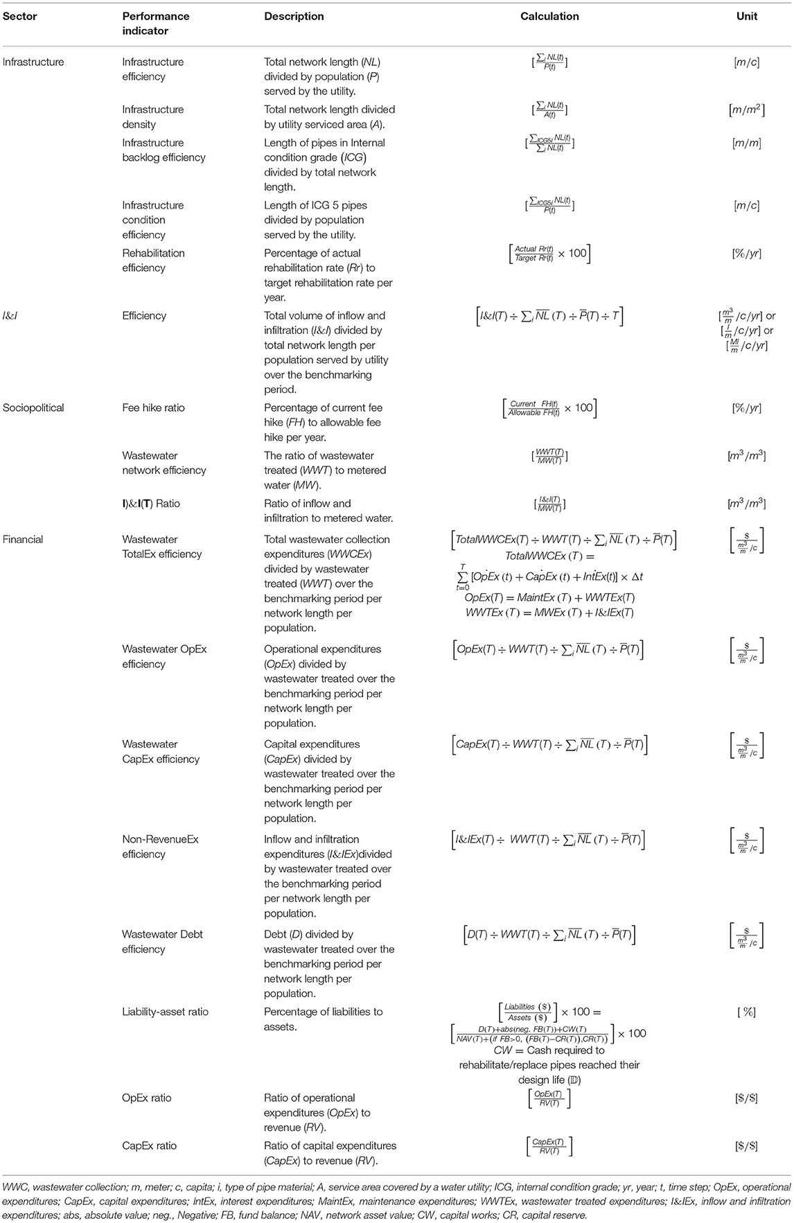
Table 1. Benchmarking performance indicators for wastewater collection networks - adopted from Ganjidoost et al. (2018).
In a separate study, Ganjidoost et al. (2021a) used the BPI's developed by Ganjidoost et al. (2018) and the concept of the three interconnected decision-making layers defined by Lloyd (2010) to develop an implementation framework for asset management strategy of water distribution networks comprised of three decision-making layers: 1) Visions & Values, 2) Function, and 3) Performance. They used an advanced system dynamics model as a Function layer to enable water utilities to plan future actions required to meet stakeholders' strategic targets and policies established in the Visions & Values layer, and benchmark and compare their performance using BPI's developed by Ganjidoost et al. (2018). Ganjidoost et al. (2021a) demonstrated the application of the entire BPI's to three water distribution networks to benchmark and compare system behavior over a 100-year benchmarking. It was found that the analyzed BPI's can improve stakeholders' understanding, support operational decisions, and thus improve performance over time. However, their work was limited to water distribution networks and the long-term performance of wastewater networks was not explored.
This study develops an implementation framework for asset management strategic planning of wastewater collection networks by advancing Rehan et al. (2014) SD model and implementing all wastewater BPI's developed by Ganjidoost et al. (2018) to quantify the current and future performance of three water utilities in Southern Ontario, Canada.
Implementation Framework of Asset Management Strategy
In conforming to the three interconnected decision-making layers defined by Lloyd (2010), this paper develops an implementation framework for the asset management strategy of the wastewater collection network comprised of three interconnected decision-making layers (Figure 1): “Visions & Values” (to find out “Where do we want to go?”), “Function” (to find out “How do we get there?”), and “Performance” (to find out “How are we doing?”). The function and merit of the proposed implementation framework for the asset management strategy of the wastewater collection network are validated using data from three water utilities in Southern Ontario, Canada. The strategic targets (see Table 2) and policy levers (see Table 3) controlling these targets are established in the Visions & Values layer. The function layer uses the advanced system dynamics model of this study, as presented in Section System Dynamics Model for Wastewater Collection Network, to achieve the visions & values of the utility. The performance layer applies the entire set of wastewater BPI's developed by Ganjidoost et al. (2018) to benchmark three independent utilities' performance and demonstrate their use. Moreover, derivative BPI's are developed to present a business case justifying the borrowing is a least total cost strategy based on the premise that the borrowing management strategy enables the utility to accelerate capital expenditures, which then improves the internal condition grade of sewer pipes. This management practice helps the utility to significantly mitigate the system's inflow and infiltration (I&I) and reduces total expenses. In fact, savings on I&I are more significant than debt expenditures for a wide range of interest rates. It should be noted that this study is limited to the linear wastewater collection pipeline.
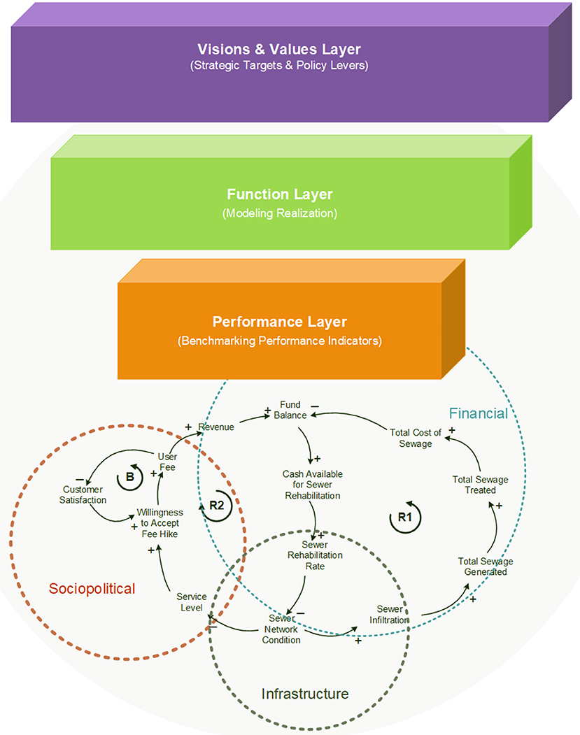
Figure 1. Implementation framework for asset management strategy of wastewater collection networks.
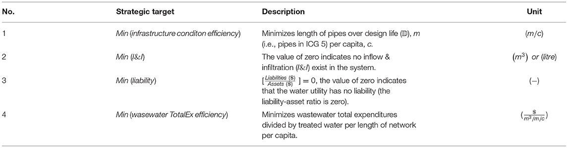
Table 2. Strategic targets for asset management strategy of the wastewater collection network.
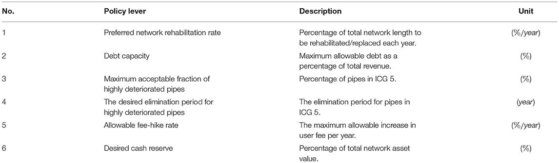
Table 3. Policy levers for asset management strategy of the wastewater collection network.
System Dynamics Model for Wastewater Collection Network
System Dynamics (SD) is a feedback-based object-oriented modeling paradigm developed by Forrester (1969) to model complex systems. Several researchers have been used SD modeling with the domain of management, water resources planning and management, construction management, economics, urban policy, etc. A detailed discussion on SD applications can be found in Richmond et al. (2001), Sterman (2000, 2001), and Ford (1999, 2000). Rehan et al. (2014) developed a system dynamics model for asset management of urban wastewater collection systems. A review of their model reveals some limitations, such as “present” vs. “future” value. This section briefly addresses the limitation associated with Rehan et al. (2014) system dynamics model. Then, improvements were made to create an advanced strategic-level asset management model corresponding to three utility's wastewater collection networks located in Southern Ontario, Canada. The advanced SD model of this study explicitly models the feedback mechanisms among the infrastructure, finance, and socio-political sectors and allows tracking of BPI's.
In system dynamics, the qualitative relationships among the various parameters influencing a system are represented through a Causal Loop Diagram (CLD). Figure 2 demonstrates a sample CLD for the management of wastewater networks to understand the complex interaction between physical, finance, and consumer sectors of the wastewater collection system. The positive or negative influence of a variable is given by the loop polarity through a plus (+) or minus (-) sign, respectively (Sterman, 2000). A positive link indicates that an increase (decrease) in one parameter causes an increase (decrease) in other parameters. Similarly, a negative link means that the dependent variable is inversely proportional to the cause, so an increase (decrease) in one variable will result in a decrease (increase) of the dependent variable(s).
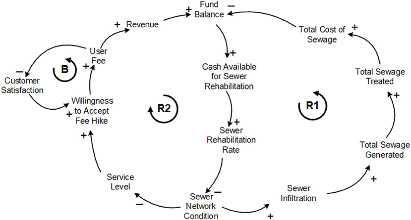
Figure 2. A causal loop diagram example for asset management strategy of wastewater collection networks.
The network condition is measured quantitatively, where an increase in network condition means pipes are deteriorating and a decrease means pipes are moving toward the best condition. Reinforcing loop R1 shows that an increase in Sewer Network Condition leads to increase in Sewer Infiltration that means more Sewage Generated and Treated, resulting the utility to spend more and leave with less cash for sewer rehabilitation. The shortfall in Cash Available for Sewer Rehabilitation causes a decrease in Sewer Rehabilitation Rate and thus an increase in Sewer Network Condition (Figure 2, R1). In a similar loop, R2 indicates that an increase in Sewer Network Condition leads to a decrease in Service Level (Figure 2, R2). A decrease in Service Level decreases customers' Willingness to Acceptance Fee Hike to pay more user fee. As User Fee decreases or remains constant, the utility will not be able to collect enough revenue and increasing Fund Balance to fund Sewer Rehabilitation programs which ultimately leads to repeatedly increasing in Sewer Network Condition. Balancing loop B shows that the satisfactory level of delivered services to customers (i.e., Customer Satisfaction) can increase (or decrease) the utility's revenue where an increase in Customer Satisfaction increases customers' Willingness to Acceptance Fee Hike and thus collecting more User Fee (Figure 2, B).
The infrastructure sector represents the inventory of pipes for the wastewater collection network. The physical condition of the wastewater collection network is divided into five variables (stocks) based upon the internal condition of the pipes using the UK's Water Research Center rating system proposed in the fourth edition of the Sewerage Rehabilitation Manual (WRc, 2001). Pipes in a given stock transfer to the next condition stock through an inflow (i.e., deterioration modeling). The condition assessment data for the wastewater collection network of each of the three utilities are collected. Moreover, the inventory of sewer pipes for the three wastewater utilities is collected and simulated in the infrastructure sector of the advanced system dynamics model. Sewage generated from different classes of customers are also incorporated into the measurements of the annual total flow; hence new sewage flow is measured not only based upon the sewage generated from the residential sector but also the sewage generated from different classes of customers such as commercial and industrial.
The finance sector describes the network's financial condition and includes revenues, expenses, fund balance, sewage fee, debt, etc. Rehan et al. (2014) assume that the unit costs are constant over the simulation period. Thus, the rate of appreciation of costs (inflation rate) is equal to the project discount rate needed to discount all costs to present value. This study incorporates inflation into the finance sector. Therefore, all costs are calculated as “future value” as the various unit costs inflate over the simulation period.
The customers of a water utility are required to pay for the treatment and collection costs associated with the amount of generated sewage flow based on their water consumption volume (Equation 1).
where, WWC wastewater collection; VC variable cost; Sf sewage fee; MW Metered water; t time; i classes of customers include residential, commercial and institutional. They are also required to pay a fixed cost for the services provided to them regardless of the amount of consumed water. This fixed cost is a function of the size of service connections (pipe's diameter) for the wastewater collection pipe (Equation 2).
where, FC fixed cost; d diameter of service connection for d = 15cm, 19cm, …, N; N maximum diameter of service connection; SSC sewage service charges; SCL service connection length. This study incorporates sewage service charges into the calculations of total revenue collected from the customers. Therefore, the wastewater collection revenue (WWCRV) is measured as the sum of variable and fixed costs as:
Developers must also pay one-time development chargers (DC) for the expenditures associated with extending wastewater collection networks to the newly developed areas. Development charges can be considered as a source of income for a wastewater utility. Still, revenue collected from customers in the form of variable and fixed costs are a significant source of income. This study incorporates development charges into the finance sector to pay capital expenditures as a source of total income. Thus, the fund balance (FB) is measured given:
where Inc income; IE interest earnings are a source of income accrued on the wastewater utility's positive fund balance (cash reserves); Sr saving rate; CapEx capital expenditures; OpEx operational expenditures; IntEx interest expenditures.
The socio-political sector presents customers' consumption behavior in response to sewage fee oscillations and the level of service delivered to them. In Rehan et al.'s (2014) model, the price elasticity of water demand is modeled as a constant parameter. In this study, the Price Elasticity of Water Demand is expanded to contain different customer classes: 1) residential, 2) commercial, and 3) institutional. Subsequently, water demand and annual water consumption and swage generated are measured and tracked based on different customer classes.
Three test methods adopted from Sterman (2000) were used to validate the SD model:
1. Structure-verification test: This test was performed to compare the structure of the model directly with the structure of the real system that the model represents. For this purpose, the model assumptions and key variables were presented and reviewed by experts from the three studied water utilities.
2. Extreme condition test: This test was conducted to check for unlikely behavior of the system in the face of extreme conditions. For this purpose, minimum and maximum values were assigned to various parameters.
3. Integration error test: This was carried out to ensure that the model results are not sensitive to the choice of a time step. Thus, simulations were conducted by cutting the time step value in half and quarter, and changes were assessed. The test results indicated no significant changes in the SD model results.
Asset Management Strategy Implementation
Three medium-sized utilities located in Southern Ontario, Canada, arbitrarily called X, Y and Z, with 341 km, 503 km, 412 km of sewer pipes that serve 120, 130, and 83 k customers, respectively, are modeled using the SD model of this study to demonstrate the application of the entire wastewater BPI's developed by Ganjidoost et al. (2018). These indicators are used to benchmark and compare the utilities' infrastructure, socio-political, and financial performance. Demographic data for each utility, including population, total length of wastewater collection pipes, and the two infrastructure BPI's of infrastructure efficiency and density, are given in Table 4. These networks are comprised of various categories of pipes made of asbestos cement (AC), polyvinyl chloride (PVC), concrete and vitrified clay (VC).
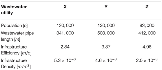
Table 4. Demographic information of wastewater utilities.
Parameters and Variables
Strategic targets and policy levers controlling these targets are made as identical as possible between each utility under the assumption they will have similar preferences to meet the utility's stakeholders' needs using a borrowing management strategy over a 100-year life cycle.
The preferred network rehabilitation rate (Policy Lever 1) is set at 1.3% of the network per year to reflect desired utility practice and target rate recommended by The Canadian Infrastructure Report Card. (2016). Policy Lever 2 allows wastewater utilities to borrow (i.e., issuing debt) up to 12.5% of their annual revenue to accelerate the capital expenditures. Policy Lever 3 is set at 10%, indicating that the utility will allow up to 10% of the length of the pipes in its wastewater collection network to be in the worst structural condition (i.e., ICG 5). If the 10% threshold is exceeded, a network rehabilitation rate higher than the preferred rate of 1.3% is required to eliminate deteriorated pipes in the network within the elimination period of 10 years (Policy lever 4). The optimal values of allowable sewage fee-hike rates (Policy Lever 5) are found to be 7% per annum for all utilities.
The current sewage fees that utilities charge their customers per cubic meter of treated wastewater are for utilities X, Y and Z, respectively. The current unit cost of wastewater treatment is reported for the three utilities. Typical average daily water consumption in the local region is 280 liters per capita per day (lpcd) for utilities X and Z and 322 lpcd for utility Y, and are used as the initial water demand for this study. The minimum water demand for the three utilities is assumed to be 150 lpcd.
The current unit cost for rehabilitating pipes in condition grade 4 (ICG 4) is reported to be $600 per meter, and for pipes in condition grade 5 (ICG 5) is set at $1000 per meter for the three utilities. The unit operation and maintenance costs and inflow and infiltration rates are calculated in a manner identical to Rehan et al. (2014). The 5.52% per annum inflation rate reported by Younis et al. (2016) for wastewater pipe construction projects is used in this study to inflate the unit cost of pipe renewal($/m), the unit cost of pipe maintenance ($/m/year), and the unit price of treated wastewater ($/m3). Household income is inflated over the benchmarking period at a rate of 2.4% per annum based on the customer price index (CPI) of Canada.
Results
The borrowing management strategy is compared over a 100-year benchmarking period using three categories of BPI's developed by Ganjidoost et al. (2018) for the wastewater collection network: 1) infrastructure, 2) socio-political, and 3) financial (see Table 1). Benchmarking results for the three wastewater utilities are illustrated in Figures 3–5.
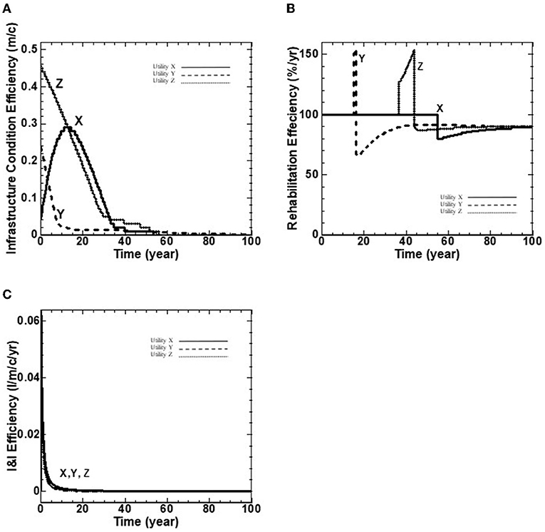
Figure 3. (A–C) Wastewater infrastructure performance indicators over a 100-year benchmarking period.
Infrastructure Performance Indicators
This category measures the infrastructure performance of the wastewater collection network. The BPI's of infrastructure efficiency and density for each utility are provided in Table 4. The model can quantify network expansion and population growth/decline. However, with respect to the three utilities inputs/insights to the model, this study assumed that the wastewater network length, population and area serviced by the utility are constant over the benchmarking period. Therefore, the infrastructure efficiency BPI is 2.84, 3.87 and 4.96 m/c, for utilities X, Y and Z, respectively, while the infrastructure density BPI is 5.3 × 10⁻³, 4.6 × 10⁻³ and 2.0 × 10⁻³ for utilities X, Y and Z, respectively, as noted in Table 4. The three BPI's of a) infrastructure condition efficiency (m/c), b) rehabilitation efficiency (%/yr), and c) I&I efficiency (l/m/c/yr) are illustrated with wastewater utilities X, Y and Z in Figure 3.
Figure 3A shows the infrastructure condition efficiency (i.e., length of ICG 5 pipes per capita) for the three wastewater utilities. For utility X, the infrastructure condition efficiency starts with a value of 0.04 m/c, increases to 0.22 m/c at 10 years due to ICG 4 pipes moving to ICG 5, then decreases to reach the value of 0.0 m/c at 45 years where it remains to the end of benchmarking period. For utilities Y and Z, the fraction of highly deteriorated pipes starts with a value of 0.24 and 0.46 m/c, respectively, followed by a decline to reach the value of 0.0 m/c at 45 years and to the end of the benchmarking period, as shown in Figure 2A.
Figure 3B shows the rehabilitation efficiency BPI. The result of this BPI indicates that the strategic target of Min (m/c), length of highly deteriorated pipes (i.e., ICG 5 pipes) per capita is met using the controlling Policy Lever of the preferred rehabilitating rate of 1.3% of the network length per year. The value above 100 percent indicates that the acceptable fraction of deteriorated pipes (Policy Lever 3) exceeds its maximum threshold of 10%. Hence, the actual network rehabilitation rate is higher than the preferred rate of 1.3% (Policy Lever 1) in order to eliminate deteriorated pipes in the network within the elimination period of 10 years (Policy Lever 4).
For Utility X, the rehabilitation efficiency starts with a value of 100 percent and remains constant for 55 years due to ICG 5 pipes. Thereafter, there is a sudden decline to reach the minimum value of 78 percent at 55 years, and then is followed by a continuous increase to 90 percent at 80 years due to aging ICG 4 pipes and remains constant to the end of the benchmarking period (Figure 2B). For Utility Y, the rehabilitation efficiency starts with a value of 100 percent, climbs to 154 percent at 12 years due to ICG 5 pipes backlogs, followed by a sudden decline to 65 percent at 13 years, and a continuous climb to 90 percent at 80 years due to ICG 4 pipes aging to ICG 5, and remains constant to the end of the benchmarking period (Figure 3B). For Utility Z the rehabilitation efficiency starts with a value of 100 percent, followed by a sudden climb to 124 percent at 38 years due to increase in the volume of ICG 5 pipes, and continues to increase to reach its maximum value of 152 percent at 43 years, followed by a sudden decline to 83 percent at 45 years, and then followed by a continues climb to 90 percent at 80 years due to ICG 4 pipes aging to ICG 5, and remains constant to the end of the benchmarking period (Figure 3B).
Figure 3C depicts the BPI of I&I Ratio by measuring the volume of I&I per meter per capita over the benchmarking period . It shows the initial values of for utilities X, Y and Z, respectively, followed by a sudden decline to their minimum values (close to zero percent) at 5 years and remains at the same value to the end of the benchmarking period. This performance indicator declines for the three utilities implying that they all achieve the strategic target of minimizing I&I over the life cycle of the infrastructure.
Socio-Political Performance Indicators
This category measures the socio-political performance of three wastewater utilities in terms of a) fee hike ratio (%/yr), b) wastewater network efficiency (m3/m3), and c) inflow and infiltration (I&I) ratio (m3/m3). The results of this category show that the three utilities achieve the stated strategic targets of Min (I&I), as shown in Figures 4B,C.
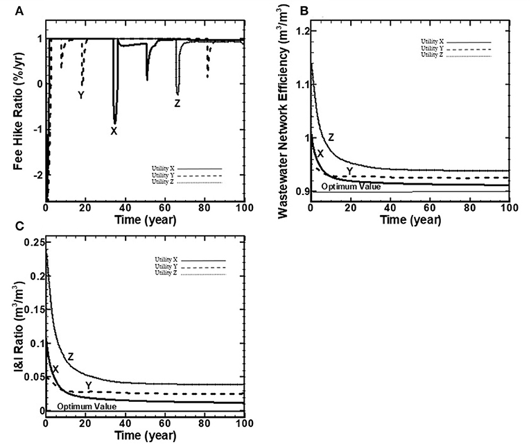
Figure 4. (A–C) Wastewater socio-political performance indicators over a 100-year benchmarking period.
Figure 4A shows the fee hike ratio BPI for the three wastewater utilities. This BPI is measured as a percentage of current to allowable fee-hike rates over the benchmarking period. A value of unity indicates that the current fee hike rate equals the allowable fee-hike rate. Fee hike ratio BPI shows some oscillations over the benchmarking period due to available funds required to pay for wastewater expenditures.
As depicted in Figure 4B, the BPI of wastewater network efficiency shows a declining trend for the three utilities. The optimum value is assumed to be 0.9 out of 1.0 based on the assumption that 0.1 (i.e., 10%) of metered water is non-consumptive water used by customers and not returned to the wastewater collection system (for instance, water used in watering lawns and evaporated from pools). Hence, a value of 0.9 indicates that the wastewater network is 100% efficient and treated wastewater equals metered water (i.e., no I&I exist in the system). The wastewater network efficiency BPI starts with a value of 1.0, 0.95 and 1.15 for utilities X, Y and Z, respectively, followed by a decline to their minimum values of 0.92, 0.94 and 0.96, respectively, at the end of benchmarking period.
Figure 4C shows the ratio of I&I to metered water over the benchmarking period. The optimum value for this performance indicator is 0.0 and indicates that there is no I&I in the system. Utility Z has the highest I&I ratio over the benchmarking period, shown in Figure 2C due to the fraction of its highly deteriorated pipes (Figure 3A) compared to the other two utilities. Ultimately, as simulated by the model, the three utilities achieve the strategic targets of Min (I&I), minimize inflow and infiltration over the benchmarking period.
Financial Performance Indicators
The financial performance of the three utilities' wastewater collection networks is benchmarked using the eight BPI's for wastewater networks developed by Ganjidoost et al. (2018). The benchmarking results, as illustrated in Figure 5, indicate that the three utilities meet the strategic targets of: Min (wastewater TotalEx efficiency), Min (I&I), and Min (liability).
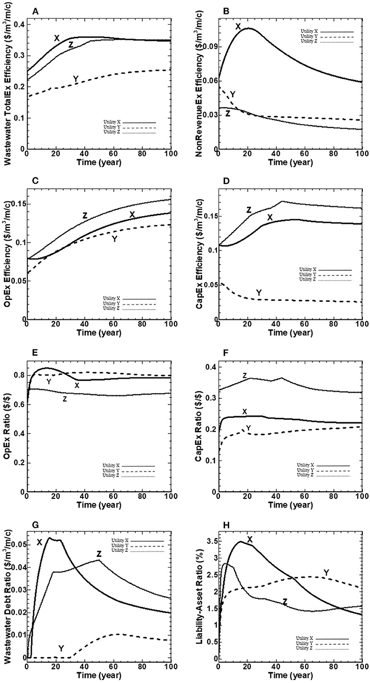
Figure 5. (A–H) Wastewater financial performance indicators over a 100-year benchmarking period.
Residents of utility X spend more dollars per cubic meter of treated wastewater per length of network per capita in the first 60 years than the other utilities, as depicted in Figure 5A. This is due to its higher value of non-RevenueEx Efficiency over the entire benchmarking period (Figure 5B), and its highest wastewater debt ratio for nearly 30 years (Figure 5G) compared to the other utilities. In contrast, residents of utility Y experience the least wastewater TotalEx efficiency values over the benchmarking period. Wastewater TotalEx efficiency starts with a value of for utilities X, Y and Z, respectively, followed by a linear increase to converge to the value of for utilities X, Y and Z, respectively (Figure 5A). The three utilities ultimately achieve similar behavior over the entire benchmarking period with the spread in their wastewater TotalEx Efficiency never separating by more than $0.19 . The spread persists due to the assumption of constant population and network length combined with the allowable fee-hike rates that permit each utility to have sufficient revenue to meet expenses over the benchmarking period. In summary, the three utilities achieve the strategic targets of minimizes total wastewater expenditures divided by treated wastewater per length of network per capita.
Figure 5B shows the non-RevenueEx Efficiency BPI that is measured in terms of I&I expenditures over treated wastewater per meter of network length per capita. It starts with the initial values of for utilities X, Y and Z, respectively. The results show a similar declining trend for utilities Y and Z to the end of the benchmarking period to reach their minimum values of . For utility X, the non-RevnueEx Efficiency increases to reach its maximum value at 20 years. Thereafter, it declines toward the end of the benchmarking period and reaches a value of (Figure 3B). In summary, the three utilities meet the strategic targets of 1) Min (wastewater TotalEx efficiency) and 2) Min(I&I) over the benchmarking period.
Figure 5C shows the OpEx efficiency BPI for the three wastewater utilities that is measured in terms of operational expenditures over treated wastewater per meter of network length per capita. The OpEx efficiency BPI starts with initial values of for utilities X, Y and Z, respectively, and continues to increase to the end of the benchmarking period to reach the value of for utilities X, Y and Z, respectively (Figure 5C).
Figure 5D shows the CapEx efficiency BPI in terms of capital expenditures over treated wastewater per meter of network length per capita. The CapEx efficiency BPI starts with the initial values of for utilities X, Y and Z, respectively (Figure 5D). The results indicate the same trend for all utilities beyond 40-50 years, with the final values of (Figure 5D). Utility Y experiences the least dollars divided by cubic meter of treated wastewater per meter per capita for its capital works compared to the other utilities due to its youngest inventory of pipes (Figure 3A). Ultimately, all utilities achieve similar behavior over the entire benchmarking period, with the spread in their CapEx efficiency never separating by more than approximately $0.15 , respectively. In summary, the three utilities achieve the strategic targets of Min (wastewater TotalEx efficiency) by minimizing capital expenditures over treated wastewater per meter of network length per capita and comply with the Policy Lever of no more than 10% of the network in ICG 5 pipes.
The OpEx ratio BPI determines whether a utility achieves its operational program targets by measuring the percentage of operational expenditures over the revenue, as noted in Table 1. Figure 5E shows the OpEx ratio for the three wastewater utilities. The OpEx ratio starts with a value of 0.61, 0.63 and 0.70 for utilities X, Y and Z, respectively, and follows with some curvatures to the end of the benchmarking period to reach the values of 0.78, 0.79 and 0.68 percent for utilities X, Y and Z, respectively.
The CapEx ratio BPI determines whether a utility achieves its capital works targets by measuring the percentage of capital expenditures over the revenue, as noted in Table 1. Water utility Z has the highest value of CapEx ratio over the benchmarking period (Figure 5F) due to the highest fraction of ICG 5 pipes (Figure 5D). Therefore, it requires spending more funds on capital works to comply with Policy Lever 3, no more than 10% of the network in ICG 5 pipes.
The wastewater debt ratio BPI, as shown in Figure 5G, measures the utility' debt expenditures divided by treated wastewater per meter of network length per capita . This indicator starts with the initial value of for the three utilities, reaches the maximum values of at 12, 60 and 50 years for utilities X, Y and Z, respectfully, and declines to the end of the benchmarking period to reach the final values of for utilities X, Y and Z, respectfully.
As depicted in Figure 5H, the BPI of liability-asset ratio is measured as a percentage of total liabilities relative to total assets for a utility. This indicator starts with the initial value of zero percent for all three wastewater utilities, follows by an increase to reach its maximum value of 3.5, 2.8 and 2.4% for utilities X, Y, and Z, respectively, and follows by a declining trend to the end of the benchmarking period to reach the value of 1.3, 1.6, and 2.1% for utilities X, Y, and Z, respectively.
Discussion
This study demonstrates the idea of how the utility's stakeholders can use the application of the entire wastewater BPI's developed by Ganjidoost et al. (2018) to understand and track the complex non-linear behavior of their system's performance over the benchmarking period. The benchmarking results indicate that the three utilities can achieve their strategic targets using the controlling policy levers established in Tables 2, 3, respectively.
The average wastewater debt ratio BPI over the benchmarking period is $0.03, $0.01 and $0.03/m3/m/c for utilities X, Y and Z, respectively, and, the average non-RevenueEx Efficiency BPI is $0.08, $0.03 and $0.03/m3/m/c for utilities X, Y and Z, respectively. Comparing the results of these two BPI's implies that a borrowing management strategy can enable the utility to significantly mitigate the volume of (I&I) and reduces its associated costs over the benchmarking period.
The borrowing management strategy can provide sufficient funds for the utility to replace its existing backlog of deteriorated sewer pipes and to maintain network rehabilitation at the preferred rate of 1.3% of the network length per year (policy lever). As a result of issuing debt, the utility's liability increases. On the other hand, capital works improve the average network condition and increase the network assets' monetary value. Ultimately the three utilities can achieve the strategic target of minimizing liability over the benchmarking period (Figure 3H).
The results show that the three utilities meet the stated strategic targets of 1) Min (infrastructure condition efficiency); 2) Min (I&I), the BPI's of I&I Efficiency, wastewater network efficiency, I&I ratio and non-RevenueEx efficiency, 3) Min (liability), the BPI of liability-asset ratio, and 4) Min (wastewater TotalEx efficiency), minimize total wastewater expenditures divided by treated wastewater per length of network per capita. Therefore, the three utilities sustainably maintain these targets using the controlling policy levers noted in Table 3 over the benchmarking period.
Effect of Interest Rate Spread on Borrowing Strategy
The previous simulations assessing the three wastewater utilities' BPI's involved an interest rate spread of 1.5% per annum above the risk-free rate (the respected utilities' rate), with a maximum issuance debt capacity of 12.5% of annual revenue. Municipal governments in Ontario, Canada, can borrow at a typical spread of 1% per annum (the respected utilities' insight) in excess of the risk-free rate established by Canada Bond. Additionally, the three utilities have an allowable fee-hike rate of 7% per annum with a 1.3% preferred network rehabilitation rate (the desired rate for the respected utilities). A key issue within this study is to assess the business case of borrowing as a financial strategy to accelerate capital expenditures, thereby minimizing operation expenditures and the total cost of the wastewater network over its design life. The viability of this business case is dependent on the spread rate. Therefore, it is instructive to explore network management strategies over a broader range of two policy levers of 1) allowable fee-hike and 2) preferred network rehabilitation rates under interest rate spread values of 0, 1.5, and 3% per annum. An interest rate spread of 0% per annum is essentially “free” money whereby the Federal government provides a grant to the utility, with repayment tied to the Federal government's ability to raise capital. In contrast, an interest rate spread of 3% per annum is slightly in excess of typical municipal bonds to investors within the US. An interest rate spread of 1.5% per annum is comparable to what Infrastructure Ontario attempts to offer to participating municipalities.
Within each scenario set (see Table 5), the allowable fee-hike rate is varied over a range of 0% to 12% per annum, and the preferred network rehabilitation rate is varied over a range of 0% to 3% per annum with a unique maximum debt capacity of 12.5% of utility's annual revenue. It is assumed that an allowable fee-hike rate in excess of 12% per annum is not a politically feasible strategy for the utility to sustain itself over the long run. Similarly, a capital works plan rehabilitating in excess of 3% of the network per year is assumed not feasible due to the availability of physical and financial resources. Policy levers for the three scenario sets are provided in Table 5. The effect of interest rate spread is presented on two selected BPI's representing infrastructure and financial performance of utilities. The BPI of infrastructure condition efficiency (m/c) is chosen for infrastructure performance and the BPI of wastewater TotalEx Efficiency ($/m3/m/c) is selected for the financial performance of the utility over the benchmarking period.
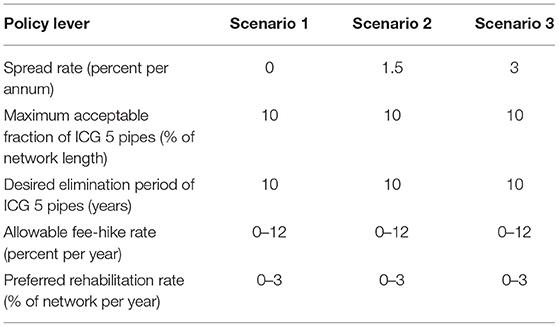
Table 5. Policy levers for three scenario sets.
Figures 6A–C present the contours of the maximum value of infrastructure condition efficiency BPI over the benchmarking period, for scenarios 1, 2 and 3 with 0, 1.5 and 3% per annum interest rate spread, respectively. These contours are the mean BPI values arising from ~4,000 simulation runs for the three utilities. For comparative purposes, utilities X, Y and Z with the unique set of allowable fee hikes and preferred network rehabilitation rates, as discussed in the previous section, are illustrated with white dots on Figures 6A–C. Figures 6D–F show contours of the wastewater TotalEx Efficiency at 100 years, as measured in terms of cumulative total wastewater collection expenditures divided by cumulative treated wastewater per length of wastewater network per capita ($/m3/m/c) at 100 years, for scenarios with 0, 1.5 and 3% per annum spread, respectively. These contours are also the mean BPI values arising from the simulations (approximately 4,000 runs) for the three utilities. Once again, for comparative purposes, utilities X, Y and Z are depicted with white dots on Figures 6D–F.
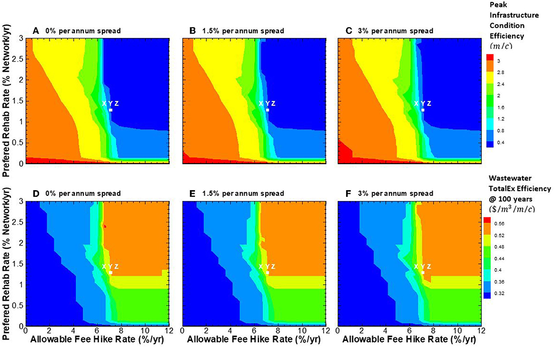
Figure 6. (A–F) Impact of allowable fee hike and preferred rehabilitation rates on infrastructure condition efficiency and wastewater TotalEx efficiency.
Figures 6A–C indicate that the maximum value of infrastructure condition efficiency BPI decreases as the allowable fee-hike rate increases to its maximum value. The results show no significant sensitivity to the maximum value of infrastructure condition efficiency as the preferred rehabilitation rate increase to its maximum value (Figures 6A–C). The results of Figures 6A–C show similar behavior with the different spread of 0, 1.5 and 3% per annum. The least (m/c) region is shown with a blue contour for a spread of 0, 1.5 and 3% per annum. From a socio-political perspective, the utility should operate on the boundary of the blue contour. The results of different spread rates indicate that the three utilities, as depicted with white dots on Figures 6A–C, operate on the boundary or in the blue region. This means Efficiency in terms of infrastructure condition for the three utilities with the unique allowable fee hike of 7% per annum and 1.3% preferred network rehabilitation rate per annum.
Figures 4D–F indicate that the value of wastewater TotalEx Efficiency, as a financial BPI, has the opposite trend relative to the infrastructure condition efficiency and increases as the allowable fee-hike rate increases over the benchmarking period. The least TotalEx efficiency region is shown with a blue contour for a spread of 0, 1.5, and 3% per annum. Figures 4D–F indicate that spread increases from 0 to 3% per annum; the wastewater TotalEx Efficiency shows similar behavior for all combinations of allowable fee-hike rate and rehabilitation rate. For the original scenarios of X, Y and Z, as shown with dots on Figures 6D–F, the results indicate that the three utilities operate on the boundary of the orange-contour region.
most important observation is that contours represent the “optimal” combination of allowable fee-hike and preferred rehabilitation rates in minimizing either the infrastructure condition efficiency, as physical infrastructure BPI or the wastewater TotalEx Efficiency, as the financial BPI has a different shape. The utility should select the optimal combinations of allowable fee-hike rate and preferred rehabilitation rate that is on the boundary of the blue region or in the light blue region for the infrastructure condition efficiency, and the optimal combinations of allowable fee-hike rate and preferred rehabilitation rate that are on the boundary of the orange region or in the yellow region for the wastewater TotalEx Efficiency. This can enable them to sustainably achieve the stated targets over the life-cycle of their infrastructure assets. It should be noted that utilities can select the optimal combinations of allowable fee-hike and preferred rehabilitation rates based upon their preferences and stakeholders' objectives.
Business Case for Asset Management of Wastewater Collection Networks
This section presents a business case for asset management of wastewater collection networks using a borrowing management strategy. The innovation of this section is to illustrate how the previous BPI's can be rearranged to yield a derivative BPI metric: Inflow and infiltration expenditures (I&IEx) saving ratio. The objective of this new BPI metric is to explore the benefits of a borrowing management strategy with the maximum debt capacity of Q% relative to a no borrowing (pay-as-you-go) management strategy (i.e., 0% debt capacity). The I&IEx saving ratio is introduced in Equation 5. It expresses the business case for borrowing by subtracting I&IEx with Q% debt capacity and its associated interest expenditures (IntEx) from I&IEx with 0% debt capacity, and further normalized by I&IEx with 0% debt capacity. The derivative BPI is expressed as:
where, I&IEx = inflow and infiltration expenditures; Dc = Debt capacity (% of annual revenue per annum); Q = maximum debt capacity (% of annual revenue per annum); t = time (year); T= benchmarking period in years; t = time step. An I&IEx saving Ratio with a value >0% supports the business case by indicating a net reduction in total expenses over the design life of the infrastructure. In contrast, an I&IEx saving ratio of <0% does not support the business case for borrowing.
It is instructive to explore the impact of borrowing vs. no borrowing management strategies over a broader range of two policy levers: 1) allowable fee-hike and 2) preferred network rehabilitation rates. These policy levers are varied in a manner analogous to the previous section over the same interest rate spread values of 0, 1.5, and 3% per annum. Maximum debt capacity (Q) is set at 12.5% of utility's annual revenue, as indicated in Table 4.
Figures 7A–C present the contours of I&IEx saving ratio over the benchmarking period, with 0, 1.5 and 3% per annum interest rate spread, respectively. These contours are the mean BPI values from the simulations (~4,000 runs) for the three utilities. For comparative purposes, utilities X, Y, and Z with a 7% allowable fee-hike rate and a 1.3% preferred network rehabilitation rate are illustrated using white dots on Figures 7A–C. The results of different interest rates spread indicate that the three utilities, as depicted with white dots on Figures 7A–C, operate on the green region with an I&IEx saving ratio value in the range of 30–50%. This indicates that the borrowing management strategy with a 12.5% debt capacity can enable the three utilities to save more on I&I expenditures, with the unique allowable fee-hike of 7% per annum and 1.3% preferred network rehabilitation rate per annum.
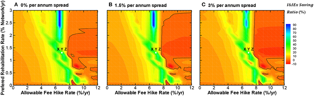
Figure 7. (A–C) Impact of allowable fee hike and preferred rehabilitation rates on I&IEx saving ratio.
There is a clear trend of issuing debt ranging from 0 to 3% per annum spread causes more interest expenditures. As the interest rate spread increases, interest expenditures also increase, causing the utility to spend a greater proportion of income on servicing debt. This prevents the utility from rehabilitating the ICG 5 pipes quickly and then slightly increasing the value of infrastructure condition efficiency BPI (i.e., length of ICG 5 pipes per capita), with a resulting increase in I&I flows. Figures 7A–C show as long as the I&IEx saving ratio remains above 0% contour line, and interest expenditures remain less than savings on I&I expenditures. In summary, issuing debt is a premier management strategy as long as the combinations of allowable fee-hike and preferred rehabilitation rates remain outside the 0% contour line, as shown in Figures 7A–C.
Conclusions
This study demonstrates a unified implementation framework for the asset management strategy of wastewater collection networks to meet sustainable infrastructure, socio-political, and financial targets over the life cycle of the infrastructure. The advanced system dynamics model enables three customized models for each independent utility to represent their infrastructure, financial and socio-political characteristics. The system dynamics model helped water utilities to plan future actions required to meet stakeholders' objectives. The application of the entire BPI's developed by Ganjidoost et al. (2018) demonstrated how water utilities could benchmark, compare and understand their system performance over the benchmarking period, proactively manage their system, and meet their strategic targets.
Based on this study, the following conclusions can be drawn:
1. An advanced system dynamics model is developed to forecast the future behavior of wastewater collection networks.
2. The output of the advanced system dynamics model is then used to demonstrate the first known application of the entire benchmarking performance indicators for wastewater collection networks developed by Ganjidoost et al. (2018).
3. A framework for asset management strategy of wastewater collection networks is developed, comprised of three decision-making layers: 1) visions & values, 2) function (i.e., advanced SD model), and 3) performance (i.e., BPI's).
4. Benchmarking results indicate that all three utilities can sustainably meet the strategic targets using the controlling policy lever over the benchmarking period.
5. The “optimal” combinations of allowable fee hikes and rehabilitation rates along with a borrowing management strategy (i.e., issuing debt) will allow utilities to accelerate capital works and sustainably meet their strategic targets over the life cycle of assets.
6. Borrowing management strategy can be a practical and long-term solution for utilities to sustainably operate and maintain their assets using the combinations of allowable fee-hike and preferred rehabilitation rates, leading to a positive value of I&IEx saving ratio.
Future works are recommended to further refine and expand the scope of the presented framework for the asset management strategy of wastewater collection networks. Further works can be done using the underlying conceptual ideas of this framework to create integrated frameworks for the asset management strategy of water, sewer, storm, and treatment plants.
For this study and with respect to the three utilities inputs/insights to the model, the wastewater network length and population serviced by the utility were assumed to be constant over the benchmarking period. From the utility's financial perspective, population growth doesn't necessarily mean more fund balance. With more new vertical developments, many network expansions cannot be expected because the new needs could be satisfied with a pipe replacement to collect and carry more sewage flow to treatment plants. The system dynamics model and framework presented in this study can be used by any utilities (regionally, nationally, or globally) with the combinations of different scenarios to provide a trend over the simulation period. However, future works can be done to explore the impacts of network expansion and population growth/decline on the utility's infrastructure, socio-political, and financial targets.
Data Availability Statement
The original contributions presented in the study are included in the article/supplementary material, further inquiries can be directed to the corresponding author/s.
Author Contributions
AG: conceptualization, methodology, data collection, modeling, software, formal analysis, visualization, and writing—original draft. AG, MK, AU, and CH: writing—review and editing. MK, AU, and CH: supervision. All authors contributed to the article and approved the submitted version.
Conflict of Interest
AG was currently an employee of Xylem and that this affiliation began after the research in the manuscript took place.
The remaining authors declare that the research was conducted in the absence of any commercial or financial relationships that could be construed as a potential conflict of interest.
Publisher's Note
All claims expressed in this article are solely those of the authors and do not necessarily represent those of their affiliated organizations, or those of the publisher, the editors and the reviewers. Any product that may be evaluated in this article, or claim that may be made by its manufacturer, is not guaranteed or endorsed by the publisher.
Acknowledgments
We gratefully acknowledge the financial support provided by the Natural Science and Engineering Council of Canada, the University of Waterloo, and the Centre for Advancement of Trenchless Technologies located at the University of Waterloo. We also acknowledge the City of Waterloo, the City of Niagara Falls, and the City of Cambridge for their financial support, provision of data, and sharing of valuable insights on water utility management.
References
Baah, K., Dubey, B., Harvey, R., and McBean, E. (2015). A risk-based approach to sanitary sewer pipe asset management. Sci. Total Environ. 505, 1011–1017. doi: 10.1016/j.scitotenv.2014.10.040
Board Governmental Accounting Standard, (1999). Statement no. 34: Basic Financial Statement and Management's Discussion and Analysis for State and Local Government.
British Standard Institution (2014). (BS ISO 55000:2014): Asset Management-Overview, Principles and Terminology (1st ed.). BSI standards.
Elsawah, H., Bakry, I., and Moselhi, O. (2016). Decision support model for integrated risk assessment and prioritization of intervention plans of municipal infrastructure. J. Pipeline Syst. Eng. Pract. 2016:04016010. doi: 10.1061/(ASCE)PS.1949-1204.0000245
Ford, A. (2000). Modeling the environment: An introduction to system dynamics modeling of environmental systems. Int. J. Sustainabil. Higher Educ. 1:002 doi: 10.1108/ijshe.2000.24901aae.002
Ford, F. A. (1999). Modeling the Environment: An Introduction to System Dynamics Models of Environmental Systems. Washington, DC: Island Press.
Ganjidoost, A., Daly, C. M., and Baird, G. (2021b). A risk-based long-term capital planning program. Pipelines 2021:3602. doi: 10.1061/9780784483602.001
Ganjidoost, A., Haas, C. T., Knight, M. A., and Unger, A. J. (2015). Integrated Asset Management of Water and Wastewater Infrastructure Systems—Borrowing From Industry Foundation Classes. In International Construction Specialty Conference of the Canadian Society for Civil Engineering. ICSC.
Ganjidoost, A., Knight, M. A., Unger, A. J. A., and Haas, C. T. (2018). Benchmark performance indicators for utility water and wastewater pipelines infrastructure. J. Water Res. Plan. Manage. 144:04018003. doi: 10.1061/(ASCE)WR.1943-5452.0000890
Ganjidoost, A., Knight, M. A., Unger, A. J. A., and Haas, C. T. (2021a). Performance modeling and simulation for water distribution networks. Front. Water 3, 718215. doi: 10.3389/frwa.2021.718215
Lloyd, C. (2010). Asset Management Whole-Life Management of Physical Assets. London: Thomas Telford Ltd.
Mashford, J., Marlow, D., Tran, D., and May, R. (2010). Prediction of sewer condition grade using support vector machines. J. Comp. Civil Eng. 25, 283–290. doi: 10.1061/(ASCE)CP.1943-5487.0000089
Mohammadifardi, H., Knight, M. A., and Unger, A. A. (2019). Sustainability assessment of asset management decisions for wastewater infrastructure systems—Implementation of a system dynamics model. Systems 7:34. doi: 10.3390/systems7030034
Rehan, R., Knight, M. A., Haas, C. T., and Unger, A. J. (2011). Application of system dynamics for developing financially self-sustaining management policies for water and wastewater systems. Water Res. 45, 4737–4750. doi: 10.1016/j.watres.2011.06.001
Rehan, R. M. A., Knight, A. J. A., and Unger, C. T. (2014). Financially sustainable management strategies for urban wastewater collection infrastructure–development of a system dynamics model. Tunnel. Underground Space Technol. 39, 116–129. doi: 10.1016/j.tust.2012.12.003
Richmond, B., Peterson, S., and Soderquist, C. (2001). STELLA: An Introduction to Systems Thinking. High-Performance Systems. Hanover: Inc.
Sterman, J. D. (2001). System dynamics modeling: Tools for learning in a complex world. Calif. Manage. Rev. 43, 8–25. doi: 10.2307/41166098
Syachrani, S., Jeong, H. S., and Chung, C. S. (2011). Dynamic deterioration models for sewer pipe network. J. Pipeline Syst. Eng. Pract. 2, 123–131. doi: 10.1061/(ASCE)PS.1949-1204.0000085
Tran, H. D., Marlow, D., and May, R. (2010). Application of Decision Support Models in Asset Management of Sewer Networks: Framework and Case Study. Pipelines 2010: Climbing New Peaks to Infrastructure Reliability, Renew, Rehab, and Reinvest.
Keywords: strategic planning, asset management, benchmarking, wastewater collection, performance modeling
Citation: Ganjidoost A, Knight MA, Unger AJA and Haas CT (2022) Performance Modeling and Simulation for Wastewater Collection Networks. Front. Water 4:723639. doi: 10.3389/frwa.2022.723639
Received: 11 June 2021; Accepted: 12 April 2022;
Published: 31 May 2022.
Edited by:
Solomon Tesfamariam, University of British Columbia, Okanagan Campus, CanadaReviewed by:
John Matthews, Louisiana Tech University, United StatesLuis-Angel Gomez-Cunya, Peruvian University of Applied Sciences, Peru
Copyright © 2022 Ganjidoost, Knight, Unger and Haas. This is an open-access article distributed under the terms of the Creative Commons Attribution License (CC BY). The use, distribution or reproduction in other forums is permitted, provided the original author(s) and the copyright owner(s) are credited and that the original publication in this journal is cited, in accordance with accepted academic practice. No use, distribution or reproduction is permitted which does not comply with these terms.
*Correspondence: Amin Ganjidoost, YW1pbi5nYW5qaWRvb3N0QHh5bGVtLmNvbQ==