 Maria Amaya
 Faye Duchin2
 John C. Little
- 1Department of Civil and Environmental Engineering, Virginia Tech, Blacksburg, VA, United States
- 2Department of Economics, Rensselaer Polytechnic Institute, Troy, NY, United States
Economic models and watershed models provide useful results, but when seeking to integrate these systems, the temporal units typically utilized by these models must be reconciled. A hydrologic-economic modeling framework is built to couple the Hydrological Simulation Program-Fortran (HSPF), representing the watershed system, with the Rectangular Choice-of-Technology (RCOT) model, an extension of the basic input-output (I-O) model. This framework is implemented at different sub-annual timesteps to gain insight in selecting temporal units best suited for addressing questions of interest to both economists and hydrologists. Scenarios are designed to examine seasonal increases in nitrogen concentration that occur because of agricultural intensification in Cedar Run Watershed, located in Fauquier County, northern Virginia. These scenarios also evaluate the selection among surface water, groundwater, or a mix of (conjunctive use) practices for irrigation within the crop farming sector in response to these seasonal impacts. When agricultural intensification occurs in Cedar Run Watershed, implementing conjunctive use in irrigation reduces the seasonal increases in nitrogen concentration to specified limits. The most efficient of the conjunctive use strategies explicitly considered varies depending on which timestep is utilized in the scenario: a bi-annual timestep (wet and dry season) vs. a seasonal timestep. This modeling framework captures the interactions between watershed and economic systems at a temporal resolution that expands the range of questions one can address beyond those that can be analyzed using the individual models linked in this framework.
Introduction
Throughout the nineenth and twentieth centuries, economic concepts have been applied in water engineering to gain insight into assessing water management concerns across different scales, such as forecasting water demand, negotiating water policy, and evaluating engineering designs (Lund et al., 2006). Water also serves as a resource used in both production and consumption, as well as a sink for the pollution byproducts of this economic activity. Thus, while water is utilized within economic systems, the impact of economic use on water quantity and quality must be considered as well (Brouwer and Hofkes, 2008). Since the 1960s and 1970s, hydrologic-economic modeling has been used by hydrologists and engineers to represent the hydrologic and economic aspects of a region within a framework (Harou et al., 2009).
In holistic hydrologic-economic models, the hydrologic and economic components of a region are incorporated into a single software package, which allows information to be easily transferred between the two systems but requires simple representations of each system (Cai et al., 2003; Brouwer and Hofkes, 2008). This approach has been applied in many studies (e.g., Cai et al., 2008; Kahil et al., 2016; Escriva-Bou et al., 2017), which focus on a comprehensive hydrologic system with some extension to economic variables. To address the lack of a complex representation of an economic system, a computable general equilibrium (CGE) modeling approach has also been utilized to capture interactions between hydrologic variables and a whole economy (Bohringer and Loschel, 2006; Brouwer and Hofkes, 2008). The CGE modeling approach is effective at capturing economy-wide impacts on hydrologic processes, but the hydrologic variables must conform to the logic of the CGE modeling framework (Scrieciu, 2007; Zhang, 2013). Thus, when these two systems are coupled in a modeling framework, typically only one system is represented in detail and extended to include variables of the other system. However, when a modular approach is applied to hydrologic-economic modeling, established models representing the different systems with adequate complexity can be coupled together, but information from each model must be correctly transformed before it can be exchanged (Cai et al., 2003; Brouwer and Hofkes, 2008; Harou et al., 2009). In the modeling framework designed by Amaya et al. (2021), the economic model, RCOT, represents resource inputs in mixed physical units and the critical linkages among economic sectors are columns of coefficients representing sectoral technologies. This input-output model is a constrained optimization model where the constraints represent physical limitations or government policies (Duchin and Levine, 2011). Thus, this model is suitable to represent the economic system in a hydrologic-economic modeling framework.
Sub-annual temporal analysis
Leontief (1970) extended the economic input-output (I-O) model to include an environmental database to evaluate the pollution generated by economic consumption and production. Since their conception, environmentally extended input-output (EEIO) databases have been used throughout the world to examine water use, waste generation, land use, and other environmental impacts resulting from economic activity. An average annual temporal resolution is commonly used in these EEIO applications since available I-O databases are typically aggregated to that scale (Sun et al., 2019). Long-term EEIO analyses have also been conducted for multi-year time periods, such as an assessment of net energy consumption in Australia over a period of 10 years (He et al., 2019) and an I-O analysis of carbon emissions from an urban region in China was also examined for a 10-year time period (Wang et al., 2019). The temporal aggregation of annual I-O tables can be misleading because it overlooks any seasonality that occurs in production throughout the year and cannot accurately evaluate unexpected events, whether natural or man-made, that generate impacts within time periods shorter than the annual scale (Donaghy et al., 2007; Avelino, 2017). A sub-annual temporal scale is important to consider to accurately estimate the environmental impacts of economic activity. However, according to Avelino (2018), the temporal disaggregation of I-O tables has had limited attention.
Temporally disaggregated I-O tables can capture the seasonal production patterns within different economic sectors, such as the agricultural sector. This seasonality in agricultural activity could also result in the time-varying distribution of resources, such as water or fertilizer, throughout the year. Temporally disaggregated, environmentally extended I-O databases could improve accuracy when incorporating environmental processes and pollution patterns into the I-O model, which operate at sub-annual time intervals (Avelino, 2017, 2018). With the possibility of linkage with a watershed model, there is also an opportunity for the sub-annual temporal analysis of water withdrawal and discharge to become more feasible within EEIO analysis (Sun et al., 2019). Thus, utilizing a hydrologic-economic modeling framework can improve the ability to choose temporal units for the economic model that are best suited to integrating the watershed model when addressing specific kinds of questions.
Conjunctive use
In many places around the globe, surface water has interactions with groundwater, which indicates that the utilization of one resource will impact the availability of the other. Surface water and groundwater have traditionally been managed as separate entities, but the potential of conjunctive water use and management has begun to be more closely examined as a solution to issues of water quantity and quality (Cobourn et al., 2017). While multiple definitions of conjunctive use are available in the literature, the definition that will be used in this paper, originally defined by the Food and Agriculture Organization of the United Nations in 1995, refers to conjunctive use as “harmoniously combining the use of (surface water and groundwater) in order to minimize the undesirable physical, environmental, and economical effects of each solution” (California Natural Resources Agency, 2016). When there is not enough surface water available for utilization, groundwater extractions tend to increase, which could lead to aquifer depletion. Conjunctive use could offer the alternative of storing surface water underground for future use when it is not practical to build storage dams (Bouwer, 2002). Mixing different sources of water could also improve water quality through blending (Ross, 2017). However, coherent water management must be clearly established to successfully implement conjunctive use policies. There must also be an adequate surplus of surface water available within a basin to exchange for groundwater. The coordination and infrastructure required to obtain, transport, and store different sources of water could also result in higher costs associated with these conjunctive use policies (Blomquist et al., 2001).
One of the largest consumers of water resources is irrigated agriculture, but this utilization is threatened by water scarcity in arid regions and excessive amounts of water for irregular time periods in coastal regions (Rao et al., 2004; Singh, 2014). Studies have been conducted on the implementation of conjunctive use for irrigated agricultural activity in these different types of regions, such as in a semi-arid region of Iran with a high level of irrigated agriculture (Montazar et al., 2010) or in the east coastal deltas of India where there is intense rice cultivation (Rao et al., 2004). In these studies, conjunctive use of surface water and groundwater was determined to be a plausible solution to optimize availability and stability of these water resources for agricultural use throughout the wet and dry periods of the year. Because there are multiple aspects that determine if conjunctive use will be successful when implemented within a region, a modeling approach is useful to evaluate and determine the most effective conjunctive use strategy for a specific region as was done by Khan et al. (2014). Utilizing a modeling framework that considers both the hydrologic and economic aspects of a region is also useful when assessing conjunctive use strategies. For example, Pulido-Velazquez et al. (2006) developed an optimization model to determine the maximum economic benefit resulting from various conjunctive management policies in Spain using several hydrologic and economic variables.
Region of study
This paper examines agricultural expansion within a regional economy, its seasonal impacts on water quality that occur within the local watershed, and the selection among conjunctive use strategies within the economic system in response to these impacts. The area of study is Fauquier County, which is in northern Virginia in the United States. This county has a long history of agricultural activity with ~54% of the county land area currently being used as farmland. Due to its proximity to the Washington DC metropolitan area, Fauquier County has also been experiencing urban development pressure. County officials are interested in preserving the rural aesthetic of the county and supporting the agricultural sector of its economy. These interests are being addressed through zoning (see Figure 1). Currently, 90% of the county is zoned for agricultural use (Rephann, 2015; Fauquier County Board of Supervisors, 2019).
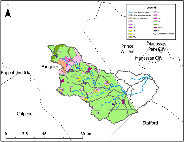
Figure 1. Zoning configuration of Fauquier County that lies within the segments of Cedar Run Watershed (outlined in solid gray). Agricultural Zones: (RA) rural agriculture, (RC) rural conservation. Non-agricultural Zones: (C-1) commercial neighborhood, (C-2) commercial highway, (CV) commercial village, (I-1) industrial park, (I-2) industrial general, (PRD) planned residential development, (R-1) residential 1 dwelling unit/acre, (R-2) residential 2 dwelling units/acre, (R-4) residential 4 dwelling unit/acre, (RR-2) rural residential, (V) village.
Within Fauquier County lies Cedar Run Watershed (498 km2), which is a sub-basin of Occoquan Watershed (1,515 km2) located 50 km southwest of Washington DC. Because algal blooms were once frequent in the Occoquan Watershed, nitrogen enrichment and eutrophication are considered primary water quality concerns for the region. As a result, both water quality and flow volume have been measured continuously within this watershed by the Occoquan Watershed Monitoring Laboratory (OWML) since 1973 (Xu et al., 2007). The Occoquan Policy was also established to regulate water quality within the Occoquan Reservoir, which is the drainage point for the Occoquan Watershed. Following this policy, the ambient nitrate concentration must not exceed 5.0 mg/L in the reservoir, otherwise nitrogen removal facilities must be activated (State Water Control Board, 2020). Thus, elevated nitrogen concentrations and increased water withdrawal caused by agricultural intensification within Cedar Run Watershed need to be carefully evaluated and utilizing a seasonal timestep within the economic system may allow for a more precise analysis.
Both urban and agricultural development are possible future development patterns in Fauquier County, but agricultural development may be more desirable to county officials for preserving the county's rural aesthetic. Therefore, the environmental implications of this development pattern are relevant to the region, especially since Cedar Run Watershed drains into Occoquan Reservoir, which serves as a source of drinking water for around two million residents in adjacent counties (Xu et al., 2007). The region is also practical due to the availability of both economic and water quality monitoring data as well as a calibrated watershed model. Specifically, an HSPF model has already been calibrated to represent the hydrologic processes of Cedar Run Watershed by OWML using local weather data collected from 2008 to 2010 and has been validated using data collected from 2011 to 2012 (Xu, 2005; Bartlett, 2013).
Research objectives
As mentioned previously, a modular hydrologic-economic modeling framework was first conceptualized by Amaya et al. (2021) to introduce the framework and demonstrate how RCOT, a physically constrained, I-O model is the most appropriate representation of an economic system to be coupled with HSPF, a deterministic, physically based watershed model using simple scenarios. In this study, these two existing models are coupled in this modeling framework to capture the seasonality of interactions between the economic and watershed systems. Addressing this new challenge requires a customization of RCOT and database as well as the design of more complex scenarios than those developed in the previous study. Specifically, the annual I-O tables utilized by RCOT are temporally disaggregated to both the bi-annual and seasonal timesteps to capture the seasonality of the environmental impacts of agricultural intensification within Cedar Run Watershed.
Several scenarios involving agricultural expansion and irrigation within Fauquier County are evaluated along with the seasonal increases in nitrogen concentration that occur within Cedar Run Watershed because of the new agricultural activity. The influence of these seasonal impacts on selections made among different conjunctive use strategies available within the crop farming sector of the economy are also examined. For these scenarios, conjunctive use is incorporated into RCOT by representing different conjunctive use strategies as nine technological options in the agricultural sector and RCOT selects the set of technologies that most efficiently meet the environmental constraints imposed by the watershed.
The disaggregation of annual economic data to seasonal and bi-annual timesteps is the objective of this study because sub-annual temporal analysis has had limited attention in the literature as previous I-O studies have focused on inter-year rather than intra-year temporal analysis (Avelino, 2017). Specifically, RCOT has been used in several studies to investigate prospects for agriculture and its reliance on land and water (i.e., Springer and Duchin, 2014; Lopez-Morales and Duchin, 2015). However, these studies do not take seasonality into account. Thus, the contribution of this paper is to develop the representation of seasons coupled with the development of alternative technologies and the representation of choices among them as well as to link it with the watershed model. By linking an I-O model, RCOT, with a continuous watershed model, HSPF, the seasonal impacts of new agricultural activity on water quality can be examined at a sub-annual temporal resolution along with how these impacts inform choices made among irrigation strategies available within the agricultural sector of the economy. In summary, the following questions will be addressed in this paper:
1. Can the introduction of conjunctive use alleviate the seasonal impacts on water quantity and nitrogen concentration caused by agricultural intensification and irrigation within Cedar Run Watershed?
2. Does a 3-month timestep produce different output results from this coupled hydrologic-economic modeling framework than when a 6-month timestep is used?
3. Does coupling a physically constrained, I-O model with a continuous watershed model provide two-way feedback that captures the interactions between the economic and watershed systems at a temporal resolution that expands the type of questions that may be addressed by either of the models coupled in this framework?
Methodology
HSPF
HSPF is a deterministic, lumped parameter, physically based model designed to continuously simulate the water quantity and quality processes that occur within a watershed at the daily timestep. In this model, the watershed system is presented as a set of constituents, such as water and pollutants, that move through a fixed environment as they interact with each other. The watershed is subdivided into elements composed of zones and nodes. Zones refer to discrete sections of the environment that may be associated with the integral of a spatially variable quantity. Nodes are defined as points in space that may be associated with a specific value of a spatially variable function and can be used to define the boundaries of zones. Thus, the relationship between zones and nodes can be described as the relationship between a function's definite integral and the values at the limits of integration. Bicknell et al. (2001) provide more detail on the processes and all the parameters utilized in HSPF.
There are two types of elements utilized by HSPF: land segments and channel reaches. Land segments are defined as areas of land with similar hydrologic characteristics. These elements are represented as layered zones in which constituents may accumulate: the soil surface layer, subsurface soil layers, and the groundwater table (see Figure 2). The constituents, such as water and nitrogen, move from one land segment downslope to another segment or channel reach. Channel reaches are one-dimensional elements represented by a single zone located between two nodes. Parameters, including flow rate and depth, are modeled at these nodes while the zones correspond with storage values that receive inflows and disperse outflows.
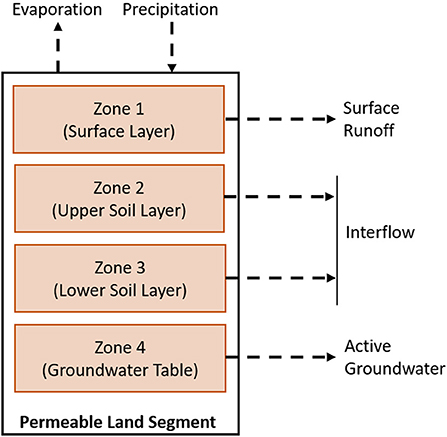
Figure 2. The zones that compose the element type, Permeable Land Segment, and the movement of the constituent (water) through the zones.
HSPF utilizes application modules to support the modeling of water quantity and quality processes that occur within the different elements. The module PERLND models the permeable land segments while RCHRES models the channel reaches. Each of these modules contain sub-modules that model the processes that occur within the corresponding elements. Within PERLND, water quantity processes are modeled using the PWATER sub-module, which models the water flow from each pervious land segment using a water budget equation to predict total runoff from pervious surfaces. The Irrigation sub-module, an addition to the PWATER sub-module, specifies source and application location of irrigation water while utilizing irrigation demand data that has been input into HSPF as an exogenously defined time series. Irrigation water may be extracted from the groundwater or channel reaches before being added to the water budget associated with each permeable land segment using the following equation where irrigation and precipitation are exogenously defined (Bicknell et al., 2001):
where,
V = volume of runoff from permeable land segment, P = precipitation, Ir = irrigation, E = evapotranspiration, G = inactive groundwater, ΔS = change in soil storage.
PQUAL, another sub-module of PERLND, is used to capture the movement and fate of water quality constituents, such as nitrogen and phosphorus, from the soil of pervious surfaces to the reaches. The deposition and flow of nitrogen through the soil of permeable land segments can be represented by the following mass balance equation where nitrogen deposition is exogenously defined (Bicknell et al., 2001):
where,
N= nitrogen stored in the soil of permeable land area, Nin= nitrogen deposition, D= nitrogen removed by decay, NOL= nitrogen removed by overland flow, NSED= nitrogen removed by detached sediment, NI= nitrogen removed by interflow, NGW= nitrogen removed by active groundwater.
HSPF also has utility modules that link the application modules and manage data. These modules utilize data that are input as time series into HSPF, such as precipitation and air temperature, to generate additional time series as output. HSPF also uses the SCHEMATIC module to exogenously specify each land segment's size and composition (Bicknell et al., 2001). The segments of Cedar Run Watershed, recognized in the HSPF model calibrated by OWML, are displayed in Figure 1.
RCOT
As an extension of the basic I-O model, RCOT contains two components: the primal quantity model and the dual price model. The primal model calculates economic output and factor use for an economy utilizing n industrial sectors and k factors of production in physical, monetary, or mixed units (Duchin and Levine, 2011). Factors of production are defined as required inputs that are not produced themselves, including labor, capital, and land. Other resources have also been incorporated into previous I-O applications as factors of production, such as water (Lopez-Morales, 2010) and nitrogen (Singh et al., 2017). Each sector of the economy has corresponding factor requirements needed to produce one unit of output. In the primal model, the basic I-O model utilizes invertible, square matrices defined by the n economic sectors, which is a feature of the EEIO sub-field as well. Uniquely, RCOT is a linear program that can select among choices in operational technologies so that specific factor constraints are satisfied. The primal model of RCOT recognizes t technologies available to the n sectors where t ≥ n. Parameters and variables, distinguished among both sectors and technologies in vectors and matrices, are denoted by an asterisk in the following equations. Thus, the matrices utilized by RCOT are rectangular rather than square. The logic utilized by RCOT is described in more detail by Duchin and Levine (2011). The following equations are used by the primal model:
where,
A*= coefficient matrix (n × t), F*= matrix of factor requirements per unit of output (k × t), y=final demand vector (n × 1), x*= economic output vector (t × 1), I*= identity matrix (n × t), ϕ= factor use vector (k × 1).
The primal model utilizes an objective function to minimize factor use while maintaining that factor use does not exceed availability and production still satisfies final demand. If the required resource endowments are unable to meet the specified consumer demand, then no feasible solution would result for a scenario. The objective function utilized by the primal model is as follows:
where,
x*= economic output vector (t × 1), y= final demand vector (n × 1), A*= coefficient matrix (n × t), f= factor endowments vector (k × 1), F*= matrix of factor requirements per unit of output (k × t), π= vector of factor prices (k × 1).
The dual price model in RCOT calculates the unit cost associated with each economic sector, based on the prices associated with each factor of production, using the following equation:
where,
π= vector of factor prices (k × 1), p= sectoral price vector (n × 1), A*′= transpose of matrix A*, F*′= transpose of matrix F*.
The dual price model of RCOT utilizes the following objective function to maximize the money value of final demand minus scarcity rents on fully utilized factors of production:
where,
y= final demand vector (n × 1), A*= coefficient matrix (n × t), I*= identity matrix (n × t), f= factor endowments vector (k × 1), F*= matrix of factor requirements per unit of output (k × t), p= sectoral prices vector (n× 1), r= factor scarcity rents vector (k× 1).
The two objective functions displayed in Equations 5 and 7 are equal at the optimal solution. This equivalence means that the total cost is equal to the sum of factor costs plus any scarcity rents. A change in the availability or unit price of a resource may result in a change in the choice selection among the technologies available to the different economic sectors (Duchin and Levine, 2011). Thus, choices in source and application of irrigation water can be introduced in the crop farming sector of the economy and then selected within the economic model based on factor price and environmental constraints.
Building the economic database
OWML has already calibrated an HSPF model to represent Cedar Run Watershed using local monitoring data collected from 2008 and 2012, but an economic database representative of Fauquier County had to be constructed for RCOT. To construct this database, sectoral economic data are obtained for the county representative of year 2012. This year serves as the base year because the most complete database that could be assembled for Fauquier County is representative of 2012. County-level, monetary, input-output data, and industry final demand data based on government data are obtained from a private company called IMPLAN Group, LLC (2016). IMPLAN obtains data from different sources and provides estimates for unavailable data, which are gauged against other data to ensure accuracy, to compile their I-O datasets. The I-O datasets obtained for this study are compiled based on annual industry accounting data collected by government agencies, such as the U.S Department of Commerce, which also produce the I-O data. Specifically, the data are compiled from the inputs reported by the firms in each economic sector. Scenarios that offer options among technologies require the development of new data to represent the requirements for each alternative technology. Thus, this development does not involve correlations but rather estimates of required inputs per unit of output.
Following the guidelines provided by Miller and Blair (2009), the I-O data obtained from IMPLAN are aggregated into seven basic industrial sectors: agriculture, mining, construction, manufacturing, utilities, professional services, and government services. These sectors are aggregated using the North American Industry Classification System (NAICS), which is recognized by the United States Census Bureau (2017). For more detailed analysis of agricultural activity, the agriculture sector is then disaggregated into three sectors as was done by Julia and Duchin (2007): crop farming, animal husbandry, and other agricultural activities. Once this data is input into RCOT, the model is run to calculate the economic output associated with each industrial sector for the 2012 base year. These output results are then assessed to ensure that the model reproduces the economic output data obtained from IMPLAN Group and to verify that this model is an accurate representation of the Fauquier County economy. Thus, Fauquier County is represented as an economic system composed of nine industrial sectors in RCOT.
To build the factor requirement (F*) matrix for RCOT, six factors of production are identified: labor, capital, land, water withdrawn, nitrogen applied as fertilizer produced outside of Fauquier County, and nitrogen applied as manure generated by the livestock associated with animal husbandry. Annual labor and capital requirements for each economic sector are calculated using sectoral data for labor, capital, and economic output obtained from IMPLAN. Sectoral land requirements are determined based on land cover data obtained from the Virginia Geographic Information Network (2016) and zoning data provided by the Fauquier County GIS Office (2014). Water withdrawal requirements for each industrial sector are determined using county water data provided by the United States Geological Survey (2010) and data obtained from an I-O database compiled by the Green Design Institute at Carnegie Mellon University (Blackhurst et al., 2010). Agricultural nitrogen requirements are assumed based on data available for Fauquier County from the National Agricultural Statistics Service (NASS). In the scenarios where conjunctive use is introduced, excess nitrogen loading is included as a seventh factor of production to distinguish between the nine irrigation strategies that are introduced. Excess nitrogen loading is defined as the increase in nitrogen loading resulting from an increase in runoff caused by the addition of irrigation water. The quantity of excess nitrogen associated with each irrigation practice is determined by running HSPF under the different irrigation configurations and incorporating this information into RCOT.
The economic database constructed to represent Fauquier County is built using data available at the annual time scale. To run the economic model at the sub-annual time scale, the final demand (y) vector and the factor requirement (F*) matrix had to be adjusted for each sub-annual timestep. HSPF begins its simulation on January 1st, 2008 and ends on December 31st, 2012. Regional cloud cover, wind speed, air temperature, and dew point temperature collected at the weather station at Washington Dulles International Airport during this 5-year period are included as input into the model at the daily timestep along with precipitation data collected at the rain gauge station located in Cedar Run Watershed. Solar radiation and potential evapotranspiration data were also input into the model during the calibration process (Xu, 2005; Bartlett, 2013). Thus, HSPF models the climate patterns that occur in Cedar Run Watershed throughout the year and their influence on the watershed. Assuming the meteorological data collected between 2008 and 2012 are typical of the study region, average watershed outflow is higher during the first 6 months of a year (January through June) than during the second 6 months (July through December). Thus, in scenarios where a 6-month timestep is used, the first timestep is referred to as the wet season and the second timestep is referred to as the dry season. In scenarios where a 3-month timestep is used, the first timestep refers to January through March (Winter), the second timestep refers to April through June (Spring), the third timestep refers to July through September (Summer), and the fourth timestep refers to October through December (Fall). The seasons are assumed to correspond with these 3-month timesteps. There is about a 10-day lag between the beginning of a season and the beginning of a month, but these approximations are reasonable for the scenarios being evaluated.
Because winter wheat and barley are listed as field crops in Fauquier County by NASS and in the report assembled by Rephann (2015), it is assumed that seasonal crop rotation is being practiced within the crop farming sector. As a result, when a 6-month timestep is used, it is assumed that the annual final demand associated with each economic sector is equally distributed among the wet and dry seasons of a year as shown in Table 1. Twenty percent of the water annually required for agricultural activity is withdrawn during the wet season and the remaining 80% is withdrawn during the dry season to compensate for high evapotranspiration rates and lower channel outflow. It is assumed that the fertilizer required for the crop farming sector is applied during the wet season while fertilizer required for animal husbandry is applied during the dry season. When a 3-month timestep is used, it is assumed that the annual final demand associated with each economic sector is equally distributed among the four seasons in a year. This assumption may be a simplification but serves for the demonstrative purposes of this study. It is assumed that 10% of the water annually required for agricultural activity is withdrawn during Winter, Spring, and Fall while the remaining 70% is withdrawn during Summer because average channel outflow is lowest during this season. It is also assumed that fertilizer required for crop farming is applied during Winter and that fertilizer required for animal husbandry is applied during Summer. Annual labor and land requirements are assumed to be constant throughout the seasons that make up the year.

Table 1. Percent of annual final demand and factor requirements utilized in each season.
Coupled modular framework
The coupled modeling framework being utilized is described in this sub-section and is visually presented in Figure 3. The economic data is downscaled from the county level to the boundaries of Cedar Run Watershed. Using a Geographic Information System (GIS), the land area of Fauquier County is overlayed with land cover data obtained from VGIN to determine the land requirements per unit of economic output for the industries present within the county. Then, the land area of Cedar Run Watershed is overlayed with land cover data. Using the land requirements determined for the industries present in the county, the economic output associated with each industry present in the watershed is determined along with the final demand for the industries in this watershed. To begin, HSPF is run under baseline conditions, which assumes no changes in the meteorological and land use characteristics that were calibrated for Cedar Run Watershed using the data measured from 2008 to 2012, before summing the resulting watershed outflow and nitrogen loading to the first timestep (either 6- or 3-month). This information is then used to determine the available quantities of factors of production in the f vector of RCOT, specifically land, water, and nitrogen. The final demand for the crop farming sector is adjusted in the y vector for the scenario being evaluated and then the economic model is run. The resulting output from RCOT includes economic output from the x vector, price per economic sector from the p vector, and the quantities of factors used to meet final demand from the ϕ vector. Information from the ϕ vector is then transferred to HSPF. Specifically, land use composition and nitrogen deposition (Nin) are exogenously adjusted within the SCHEMATIC and PQUAL modules of HSPF, respectively. Changes in water demands for irrigation (Ir) are also input as a time series in the Irrigation module.
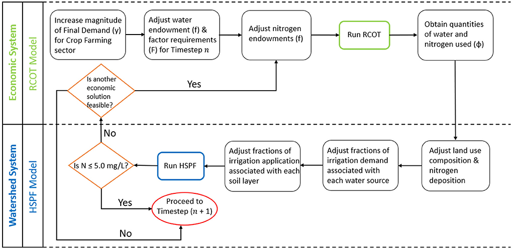
Figure 3. Decision tree representing steps taken within RCOT and HSPF during Timestep (n).
The quantity of water demanded for irrigation must be disaggregated from the 6-month (or 3-month) to the daily timestep to be input into HSPF. Since water withdrawal is assumed to be constant throughout a season, the volume of water demanded for each timestep is equally distributed among the days that make up that season. The quantity of applied nitrogen must also be input into HSPF at the monthly application rate. It is assumed that nitrogen from fertilizer is applied as nitrates (NO) and nitrogen from manure is applied as ammonia (NH3). It is also assumed that nitrogen applied as fertilizer to cropland is input during the month of March while nitrogen applied as fertilizer to pasture is input during the month of August. The sources of irrigation withdrawal are specified within the Irrigation module of HSPF along with the fractions of irrigation demand associated with each source. The fractions of irrigation demand associated with each soil layer are also specified in the Irrigation module. Once all information has been transferred to the modules of HSPF, the model is run again to obtain the watershed results for the scenario being evaluated. The water flow volumes and nitrogen loading results produced by HSPF are again summed to the first timestep.
The objective in these scenarios (characterized in Table 2) is to achieve an average nitrogen concentration of 5.0 mg/L or less in the watershed outflow during each timestep to minimize the contribution of this sub-basin to any changes in water quality within Occoquan Reservoir. If this target concentration is not reached, then the nitrogen endowments within the f vector of the economic model are adjusted before running the economic and watershed models again. The coupled models might go through multiple iterations until either the desired nitrogen concentration is achieved in HSPF, or no other feasible solution can be achieved by the economic model, before continuing to the next timestep.

Table 2. Scenario characteristics.
Scenarios
An economic database is assembled to represent Fauquier County under 2012 baseline conditions (see Section Building the economic database). Local monitoring data, collected from 2008 to 2012 has been used to calibrate an HSPF model to represent Cedar Run Watershed by OWML (Bartlett, 2013). Utilizing this data in the coupled hydrologic-economic framework described in Section Methodology, four scenarios are developed to analyze the seasonal impacts of agricultural intensification and irrigation on watershed health. Specifically, the impacts of standard irrigation are compared to the impacts of seasonal conjunctive use in irrigation on water quantity and nitrogen concentration within the outflow of the watershed. The simulation period utilized for these scenarios is 5 years, aligning with the watershed model, which utilizes meteorological data input into the model as a time series over a period of 5 years. Assuming the economy does not experience any significant change over this 5-year period, the annual final demand associated with each economic sector is not varied during the simulation period. Seasonal averages are obtained from the scenario results produced by the modeling framework over the 5 years.
These scenarios, characterized in Table 2 and described in more detail in the following sub-sections, are dramatizations based on assumptions about future human activities within Cedar Run Watershed and developed using the Fauquier County database. New agricultural activity is assumed to use irrigation so that the amount of water being removed from the watershed is increased by several orders of magnitude when compared to base year conditions, which made future watershed conditions more extreme but still plausible for Fauquier County. While these scenarios are designed for Fauquier County, they are used to demonstrate the capabilities of the coupled modeling framework, which is intended to be generalizable and used to represent other locations with different water management issues.
Standard irrigation (S1 and S2)
Under Scenarios 1 and 2 (referred to as S1 and S2 in Table 2), it is assumed that agricultural intensification has occurred within Cedar Run Watershed because of an increase in production for export. The final demand associated with the crop farming sector within the economic system is increased so that all land currently zoned for agricultural activity within the watershed is converted to cropland. It is assumed that all new economic activity is equally distributed among the land segments that make up the watershed and that water is extracted from these segments to be used for agricultural irrigation. Only one irrigation practice is available to the crop farming sector under S1 and S2 because no alternative practices are considered in these scenarios (t = n). Specifically, groundwater is withdrawn and applied to the soil surface of the cropland for irrigation use because groundwater is currently the primary source of water within Fauquier County and wells are already present within Cedar Run Watershed. It is also assumed that 40% of the irrigation water applied to the soil surface is intercepted by the crops, which is the value provided by Bicknell et al. (2001) in the HSPF manual. Thus, this irrigation practice is referred to as Standard Irrigation under S1 and S2 in Table 2.
Under S1, a 6-month timestep is used (see Table 1). It is assumed that 20% of annual water demand is withdrawn during the wet season and 80% of annual water demand is withdrawn during the dry season. It is also assumed that fertilizer for cropland is applied during the month of March, which is part of the wet season, because this month is assumed to be the time of transition between the winter and summer crops. It is assumed that fertilizer for pasture is applied during the month of August, which lies within the dry season. Under S2, a seasonal (3-month) timestep is used instead of a bi-annual timestep. It is assumed that 10% of annual water demand is withdrawn during Winter, Spring, and Fall while the remaining 70% of annual water demand is withdrawn during Summer. It is also assumed that fertilizer for cropland is applied during March, which is part of Winter, and fertilizer for pasture is applied during August, which is part of Summer. Under S1 and S2, it was expected that nitrogen concentration would be increased in the watershed outflow during the wet season and Winter, respectively, because of the fertilizer application and it was also expected that a higher temporal resolution would produce more precise results.
Implementation of conjunctive use (S3 and S4)
Under Scenarios 3 and 4 (referred to as S3 and S4 in Table 2), because of an increase in agricultural production, the final demand associated with crop farming is increased so that all land currently zoned for agricultural activity within the watershed is converted to cropland. A bi-annual timestep is utilized under S3 and a seasonal timestep is utilized under S4. Under these scenarios, conjunctive use is introduced into the crop farming sector. Specifically, alternative irrigation strategies are made available to one of the agricultural sectors represented within RCOT. As a result, the number of technologies (t) exceeds the number of sectors (n) present in the economic model (t ≥ n). The primary goal of conjunctive management is to optimize availability and stability of water resources by simultaneously managing groundwater and surface water. Thus, three water sources (groundwater, surface water, or an external water source), distinguished by different factor endowments, specifically water and nitrogen, and three choices in the irrigation location (soil surface, lower soil layer, and active groundwater table) are introduced into RCOT. When water is applied to the soil surface, it is assumed that water is sprayed from above the crop canopy. When water is applied to the subsurface, a buried irrigation system is used to uniformly release water into the lower soil layer or seep water into the active groundwater table, which ensures that water reaches the crop roots more efficiently than if it were applied on the soil surface. As a result, nine irrigation options, differing in water source and application location of the irrigation water, are available within the crop farming sector as follows (irrigation source/application location):
1. Groundwater/Soil Surface
2. Groundwater/Lower Soil Layer
3. Groundwater/Active Groundwater Table
4. Surface Water/Soil Surface
5. Surface Water/Lower Soil Layer
6. Surface Water/Active Groundwater Table
7. External Water/Soil Surface
8. External Water/Lower Soil Layer
9. External Water/Active Groundwater Table
These nine irrigation options are also differentiated based on factor price. It is assumed that groundwater is the cheapest source of water since groundwater wells are already being used within the county. An external source of irrigation water is assumed to be the most expensive. Applying irrigation water to the surface layer is assumed to be cheaper than applying the water deeper into the soil layer. There is also an increase in nitrogen loading that is generated because of the excess runoff caused by the implementation of these different irrigation practices. The largest increase in nitrogen loading results from utilizing an external water source for irrigation and the smallest increase results from utilizing surface water for irrigation. These quantities decline as the irrigation is applied deeper into the soil layers and they also vary depending on the season. In these scenarios, it was expected that the source of irrigation water would switch from groundwater to another water source to meet agricultural demand during the first timestep while groundwater would still be used during the other timesteps. Application location was also expected to switch to the sub-surface during the first timestep to minimize the excess nitrogen loading that would occur because of irrigation applied to the soil surface.
Results
Scenario results included those produced by the F vector of the economic model (see Table 3), which are obtained using a version of the RCOT model programmed using LINGO software (Springer et al., 2011). The results produced by the F vector under S3 and S4 are the same as those produced under S1 and S2, respectively, so only the results for S1 and S2 are shown in Table 3. As a result of agricultural intensification throughout the watershed, cropland increases by 280% when compared to 2012 base year conditions while jobs increase by 7.8%. Under S1, the quantities of withdrawn water and applied nitrogen increase during the wet season by 86 and 280%, respectively. During the dry season, the quantities of withdrawn water and applied nitrogen increase by 650 and 32%, respectively. Under S2, the quantity of withdrawn water increases by 185% during Winter, Spring, and Fall. During Summer, the quantity of withdrawn water increases by 1,303%. The quantity of applied nitrogen increases by 280% during Winter and by 32% during Summer.
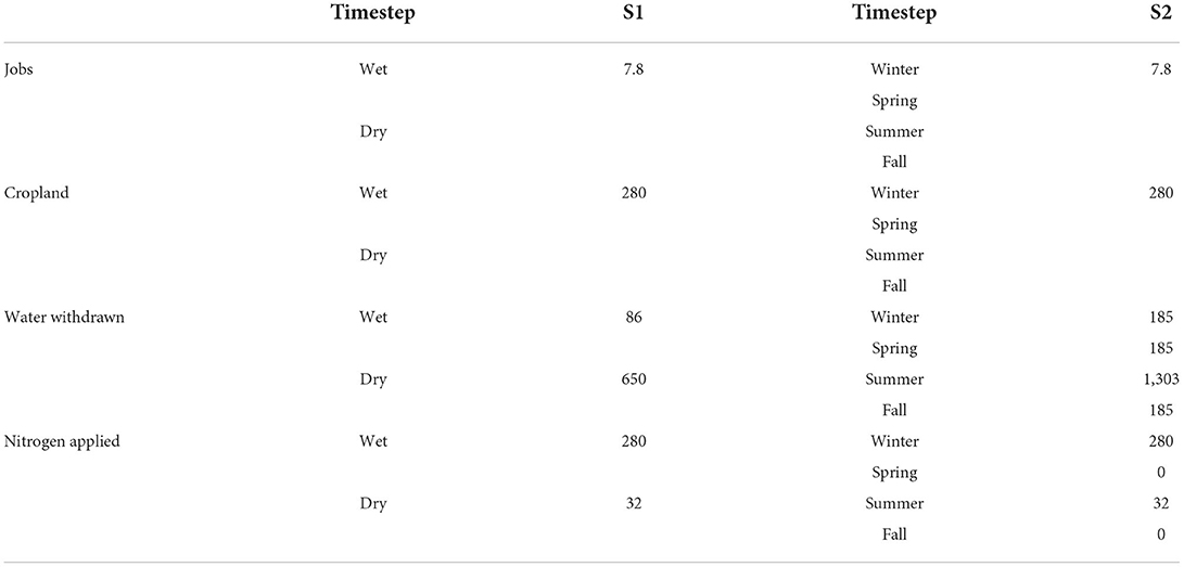
Table 3. Percent (%) increase in factor usage relative to 2012 base year.
Under S1 and S2, 100% of irrigation water is supplied by groundwater and applied to the soil surface during all timesteps. Additional results include the source and application location of irrigation water selected by RCOT under S3 and S4, which implement conjunctive use (see Table 4). Because RCOT is coupled with HSPF, the environmental impacts caused by agricultural expansion in Cedar Run Watershed are captured at the bi-annual and seasonal temporal scales. When choices of conjunctive use are implemented, irrigation strategies are introduced into RCOT, the environmental constraints imposed by the watershed system cause adjustments in management practice within the economic system, which alleviate these seasonal impacts on water quality. Under S3, groundwater applied to the soil surface is utilized during the dry season. During the wet season, 65% of irrigation is supplied by surface water while the remaining 35% is supplied by water imported from outside Cedar Run Watershed. Thirteen percent of this irrigation water is applied to the lower soil layer while the remaining 87% is applied directly into the active groundwater table. Under S4, groundwater applied to the soil surface is utilized during all seasons except Winter. During Winter, 65% of irrigation demand is supplied by surface water while the remaining 35% is supplied by a water source external to Cedar Run Watershed. Almost all the irrigation water (99%) is applied directly into the active groundwater table during Winter.
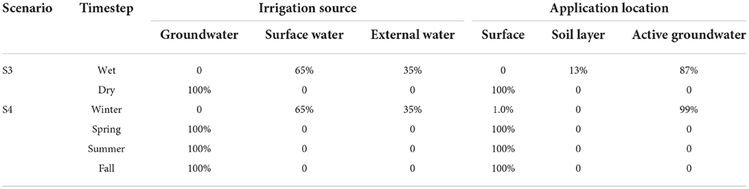
Table 4. Source and application location of irrigation water during each season.
Additional scenario results include those produced by HSPF (see Table 5), specifically the change in total watershed outflow, caused by the implementation of different irrigation strategies, and the average nitrogen concentration in that outflow. Under S1, during the wet season, the average nitrogen concentration increases to 21 mg/L in the watershed outflow while the total outflow reduces by 5.8% because groundwater is exposed to evapotranspiration. Under S2, during Winter, the average nitrogen concentration increases to 35 mg/L in the watershed outflow while the total outflow reduces by 7.4%. During the wet season under S3, the average nitrogen concentration increases to only 5.0 mg/L in the watershed outflow while the outflow quantity increases by 133% due to the use of external water when conjunctive use is implemented. Finally, during Winter under S4, the average nitrogen concentration also increases to only 5.0 mg/L in the watershed outflow while the outflow quantity increases by 156% when conjunctive use is implemented. As indicated by S1 and S2, expanded agricultural activity, irrigated using groundwater applied to the soil surface, causes an increase in nitrogen concentration at the outflow of the watershed during the first timestep, which is unexpectedly high when compared to the other seasons. S3 and S4 indicate that the introduction of conjunctive use allows the increase in nitrogen concentration to be greatly reduced during the first timestep, which is the expected outcome.
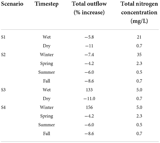
Table 5. Percent increase in total watershed outflow and average total nitrogen (TN) concentration in outflow.
Discussion
The implementation of conjunctive use alleviates the seasonal elevations in nitrogen concentration caused by agricultural intensification and irrigation in Cedar Run Watershed. Under S1 and S2, the nitrogen concentration within the watershed outflow increases significantly during the first timestep (21 and 35 mg/L, respectively) because fertilizer is applied to the soil surface and, during some years, the surface runoff is high enough during that season to wash off the fertilizer into the channel reaches. Specifically, nitrogen concentration increases significantly when fertilizer is applied during times of high flow rates within the watershed. Because of the unusually high concentration of nitrogen present in the groundwater, the utilization of groundwater irrigation also further increases the nitrogen concentration in the watershed outflow during the first timestep. This high nitrogen concentration in the groundwater could be caused by failing septic systems resulting from aging infrastructure, which have been cited as an issue in Fauquier County (Fauquier County Board of Supervisors, 2019). Applying irrigation water to the soil surface, as is done under S1 and S2, also results in an increase in surface runoff, which also contributes to the increase in nitrogen loading into the watershed outflow during the first timestep. When conjunctive use is introduced under S3 and S4, the nitrogen concentration in the watershed outflow is significantly reduced to 5.0 mg/L in the first timestep when compared to the results of S1 and S2, respectively. This reduction occurs because surface and externally sourced water applied to the subsurface of the cropland is selected among the alternatives explicitly considered as the most efficient solution to satisfy the objective functions during the first timestep. Specifically, this selection in irrigation practice minimizes the nitrogen runoff generated by the crop farming sector of the economy.
Increasing the temporal resolution to a seasonal timestep produces different results than a bi-annual timestep. When a bi-annual timestep is utilized under S3, the concentration of nitrogen in the outflow of Cedar Run Watershed can achieve a nitrogen concentration of 5.0 mg/L, which was specified as the objective for the coupled modeling framework. When a seasonal timestep is utilized under S4, the concentration of nitrogen in the outflow of Cedar Run Watershed can also meet the raw water requirement during Winter, but different conjunctive use strategies are identified as the most efficient of those considered when different sub-annual timesteps are used. Under both S3 and S4, nitrogen is applied to the cropland during the month of March, but the lower temporal resolution under S3 results in the dilution of this applied nitrogen across a 6-month period rather than a 3-month period as was the case under S4. Thus, the resolution of the sub-annual timestep must be carefully considered when coupling the economic and watershed models because the implications of different management decisions will vary depending on the timestep that is selected.
New agricultural activity can require a time-varying distribution of resources, such as water and applied nitrogen, which results in varying impacts on watershed health depending on the time of the year and depending on the management practices selected within the agricultural sector of the economy. The nitrogen concentration increases significantly during one season and then remains low during the remainder of the year. Capturing these seasonal environmental impacts on watershed health requires the temporal disaggregation of I-O data tables, but available databases tend to be aggregated to the annual time scale (Sun et al., 2019). As a result, previous I-O studies have focused on inter-year temporal development rather than intra-year temporal scales (Avelino, 2017). However, RCOT has unique features that allow for management options for all economic sectors and minimize the use of resources based on environmental constraints imposed by the watershed, which grounds human decisions in a region's physical reality (Amaya et al., 2021). By coupling RCOT with HSPF, a continuous watershed model, the seasonal environmental impacts caused by economic activity within the local watershed can be determined, which is information that cannot be obtained from either model alone. In this study, the nitrogen concentration significantly increases during Winter because of agricultural intensification. This change in nitrogen concentration is reduced to specified limits when conjunctive use is implemented within the economic system during Winter. Coupling these models at a sub-annual temporal scale captures the seasonality of interactions between the economic and watershed systems. These interactions are captured at a level of temporal detail that expands the range of questions that can be addressed by both economists and hydrologists beyond those that can be analyzed using these models individually. However, it is necessary to consider the uncertainty intrinsic in these models, such as the uncertainty associated with the empirical relationships between variables and the uncertainty of the assumptions (Settre et al., 2016). These uncertainties might be compounded when these models are coupled, but some uncertainty could be removed since assumptions may be better informed using this framework. In these initial studies, this modeling framework serves its intended purpose and future studies can be untaken to reduce uncertainty.
Conclusions
The intensification of irrigated agriculture has seasonal impacts on nitrogen concentration within the outflow of Cedar Run Watershed. Conjunctive use is a viable management practice to alleviate the seasonality of nitrogen concentration elevation caused by the expansion of agricultural activity within Cedar Run Watershed. When coupling watershed and economic systems, the temporal units must be carefully considered because the implications of different management decisions will vary depending on the timestep that is selected. If economic I-O data is collected at sub-annual temporal scales, then this modeling framework can provide insight into the interactions between watershed and economic systems at temporal units best suited for questions being addressed in empirical studies.
Future work
The coupled hydrologic-economic modeling framework will be applied to other locations with critical environmental issues and an economy that is different from that of Fauquier County. This modeling framework could also be used to examine the impacts of changing climate conditions on the coupled watershed and economic systems. Full-scale empirical studies using the WTM/RCOT model, developed by Duchin and Levine (2012), coupled with a watershed model like HSPF, would make it possible to study a region, such as Chesapeake Bay Watershed, by representing the ensemble of sub-watershed economic regions, the economic relations among them, and their interactions with the watershed at a suitable temporal resolution. For future studies, models representing the social system will also be integrated into this coupled modeling framework since this modular framework is appropriate for a system-of-systems approach that incorporates different models from different disciplines to better represent a socio-environmental system and inform policy decisions (Little et al., 2016, 2019; Iwanaga et al., 2021).
Author contributions
JL supervised the project. JL and FD conceived of the original idea. FD developed the economic model, RCOT, which is coupled with HSPF in this research. MA designed the coupled modeling framework and assembled the economic database. MA developed and modified the scenarios with the support of FD, EH, and JL, who all provided substantial input. MA drafted the manuscript and designed the figures with feedback and revisions provided by FD, EH, and JL. All authors have read and agreed to the published version of the manuscript.
Funding
We acknowledge funding from National Science Foundation Award EEC 1937012.
Acknowledgments
We would like to express our gratitude to Dr. Adil Godrej, the staff, and students at Occoquan Watershed Monitoring Laboratory for their generous cooperation and for their ongoing data collection and modeling work, which made this research study possible. This manuscript is part of MA doctoral dissertation and the co-authors include her doctoral advisor (JL) and other committee members (FD and EH).
Conflict of interest
The authors declare that the research was conducted in the absence of any commercial or financial relationships that could be construed as a potential conflict of interest.
Publisher's note
All claims expressed in this article are solely those of the authors and do not necessarily represent those of their affiliated organizations, or those of the publisher, the editors and the reviewers. Any product that may be evaluated in this article, or claim that may be made by its manufacturer, is not guaranteed or endorsed by the publisher.
References
Amaya, M., Baran, A., Lopez-Morales, C., and Little, J. C. (2021). A coupled hydrologic-economic modeling framework for scenario analysis. Front. Water 3, e681553. doi: 10.3389/frwa.2021.681553
Avelino, A. F. T. (2017). Disaggregating input-output tables in time: the temporal input-output framework. Econ. Syst. Res. 29, 313–334. doi: 10.1080/09535314.2017.1290587
Avelino, A. F. T. (2018). Essays on production chains and disruptions: New input-output perspectives on time, scale, and space. (Doctor of Philosophy). University of Illinois at Urbana-Champaign, Urbana, Illinois, United States of America.
Bartlett, J. A. (2013). Heuristic optimization of water reclamation facility nitrate loads for enhanced reservoir water quality. (Doctor of Philosophy). Manassas, VA: Virginia Polytechnic Institute and State University.
Bicknell, B. R., Imhoff, J. C., Kittle, J. L., Jobes, T. H., and Donigian, A. S. (2001). Hydrological simulation program - fortran (HSPF) user's manual, 12 Edn. Mountain View, CA: U. S. Environmental Protection Agency.
Blackhurst, M., Hendrickson, C., and Vidal, J. S. (2010). Direct and indirect water withdrawals for U.S. industrial sectors. Environ. Sci. Technol. 44, 2126–2130. doi: 10.1021/es903147k
Blomquist, W., Heikkila, T., and Schlager, E. (2001). Institutions and conjunctive use management among three western states. Nat. Resour. J. 41, 653–683.
Bohringer, C., and Loschel, A. (2006). Computable general equilibrium models for sustainability impact assessment: status quo and prospects. Ecol. Econ. 60, 49–64. doi: 10.1016/j.ecolecon.2006.03.006
Bouwer, H. (2002). Integrated water management for the 21st century: problems and solutions. J. Irrig. Drainage Eng. 128, 193–202. doi: 10.1061/(ASCE)0733-9437(2002)128:4(193)
Brouwer, R., and Hofkes, M. (2008). Integrated hydro-economic modelling: approaches, key issues and future research directions. Ecol. Econ. 66, 16–22. doi: 10.1016/j.ecolecon.2008.02.009
Cai, X., McKinney, D. C., and Lasdon, L. S. (2003). Integrated hydrologic-agronomic-economic model for river basin management. J. Water Resour. Plan. Manag. Asce 129, 4–17. doi: 10.1061/(ASCE)0733-9496(2003)129:1(4)
Cai, X. M., Ringler, C., and You, J. Y. (2008). Substitution between water and other agricultural inputs: implications for water conservation in a River Basin context. Ecol. Econ. 66, 38–50. doi: 10.1016/j.ecolecon.2008.02.010
California Natural Resources Agency (2016). Conjunctive Management and Groundwater Storage. Available online at: https://cawaterlibrary.net/document/conjunctive-management-and-groundwater-storage/ (accessed December 1, 2021).
Cobourn, K. M., Elbakidze, L., and Ghosh, S. (2017). Conjunctive water management in hydraulically connected regions in the Western United States. Compet. Water Resour. Exp. Manag. Approaches US Europe 2017, 278–297. doi: 10.1016/B978-0-12-803237-4.00016-1
Donaghy, K. P., Balta-Ozkan, N., and Hewings, G. J. D. (2007). Modeling unexpected events in temporally disaggregated econometric input-output models of regional economies. Econ. Syst. Res. 19, 125–145. doi: 10.1080/09535310701328484
Duchin, F., and Levine, S. H. (2011). Sectors may use multiple technologies simultaneously: the rectangular choice-of-technology model with binding factor constraints. Econ. Syst. Res. 23, 281–302. doi: 10.1080/09535314.2011.571238
Duchin, F., and Levine, S. H. (2012). The rectangular sector-by-technology model: not every economy produces every product and some products may rely on several technologies simultaneously. J. Econ. Struct. 1, 3. doi: 10.1186/2193-2409-1-3
Escriva-Bou, A., Pulido-Velazquez, M., and Pulido-Velazquez, D. (2017). Economic value of climate change adaptation strategies for water management in Spain's Jucar Basin. J. Water Resour. Plan. Manag. 143, 735. doi: 10.1061/(ASCE)WR.1943-5452.0000735
Fauquier County Board of Supervisors (2019). Chapter 8: Rural Land Use Plan. Available online at: https://www.fauquiercounty.gov/home/showdocument?id=7216 (accessed November 29, 2021).
Fauquier County GIS Office (2014). Fauquier County Zoning GIS Data [GIS shape files]. Warrenton, VA. Available online at: https://www.fauquiercounty.gov/government/departments-a-g/gis-mapping/gis-data (accessed May 10, 2021).
Harou, J. J., Pulido-Velazquez, M., Rosenberg, D. E., Medellin-Azuara, J., Lund, J. R., and Howitt, R. E. (2009). Hydro-economic models: concepts, design, applications, and future prospects. J. Hydrol. 375, 627–643. doi: 10.1016/j.jhydrol.2009.06.037
He, H., Reynolds, C. J., Li, L., and Boland, J. (2019). Assessing net energy consumption of Australian economy from 2004-05 to 2014-15: environmentally-extended input-output analysis, structural decomposition analysis, and linkage analysis. Appl. Energy 240, 766–777. doi: 10.1016/j.apenergy.2019.02.081
IMPLAN Group LLC. (2016). IMPLAN 2011-2013 Fauquier County Data [Data sets and Excel sheets]. Available online at: https://implan.com (accessed May 10, 2021).
Iwanaga, T., Wang, H.-H., Hamilton, S. H., Grimm, V., Koralewski, T. E., Salado, A., et al. (2021). Socio-technical scales in socio-environmental modeling: managing a system-of-systems modeling approach. Environ. Model. Soft. 135, 104885. doi: 10.1016/j.envsoft.2020.104885
Julia, R., and Duchin, F. (2007). World trade as the adjustment mechanism of agriculture to climate change. Climate Change 82, 393–409. doi: 10.1007/s10584-006-9181-8
Kahil, M. T., Ward, F. A., Albiac, J., Eggleston, J., and Sanz, D. (2016). Hydro-economic modeling with aquifer-river interactions to guide sustainable basin management. J. Hydrol. 539, 510–524. doi: 10.1016/j.jhydrol.2016.05.057
Khan, M. R., Voss, C. I., Yu, W., and Michael, H. A. (2014). Water resources management in the Ganges Basin: a comparison of three strategies for conjunctive use of groundwater and surface water. Water Resour. Manag. 28, 1235–1250. doi: 10.1007/s11269-014-0537-y
Leontief, W. (1970). Environmental repercussions and the economic structure: an input-output approach. Rev. Econ. Stat. 52, 262–271. doi: 10.2307/1926294
Little, J. C., Hester, E. T., and Carey, C. C. (2016). Assessing and enhancing environmental sustainability: a conceptual review. Environ. Sci. Technol. 50, 6830–6845. doi: 10.1021/acs.est.6b00298
Little, J. C., Hester, E. T., Elsawah, S., Filz, G. M., Sandu, A., Carey, C. C., et al. (2019). A tiered, system-of-systems modeling framework for resolving complex socio-environmental policy issues. Environ. Model. Software 112, 82–94. doi: 10.1016/j.envsoft.2018.11.011
Lopez-Morales, C. (2010). Policies and technologies for sustainable use of water in Mexico: A scenario analysis. (Doctor of Philosophy). Rensselaer Polytechnic Institute, Troy, New York, NY, United States.
Lopez-Morales, C., and Duchin, F. (2015). Economic implications of policy restrictions on water withdrawals from surface and underground sources. Econ. Syst. Res. 27, 154–171. doi: 10.1080/09535314.2014.980224
Lund, J. R., Cai, X. M., and Characklis, G. W. (2006). Economic engineering of environmental and water resource systems. J. Water Resour. Plan. Manag. Asce 132, 399–402. doi: 10.1061/(ASCE)0733-9496(2006)132:6(399)
Miller, R. E., and Blair, P. D. (2009). “The aggregation problem: level of detail in input-output tables,” in Input-Output Analysis: Foundations and Extensions, 2 Edn (New York, NY: Cambridge University Press), 160–167.
Montazar, A., Riazi, H., and Behbahani, S. M. (2010). Conjunctive water use planning in an irrigation command area. Water Resour. Manag. 24, 577–596. doi: 10.1007/s11269-009-9460-z
Pulido-Velazquez, D., Andreu, J., and Sahuquillo, A. (2006). Economic Optimization of Conjunctive Use of Surface Water and Groundwater at the Basin Scale. Journal of Water Resources Planning and Management 132, 454–467. doi: 10.1061/(ASCE)0733-9496(2006)132:6(454)
Rao, S. V. N., Bhallamudi, S. M., Thandaveswara, B. S., and Mishra, G. C. (2004). Conjunctive use of surface and groundwater for coastal and deltaic systems. J. Water Resour. Plan. Manag. Asce 130, 255–267. doi: 10.1061/(ASCE)0733-9496(2004)130:3(255)
Rephann, T. J. (2015). Fauquier County Cost of Community Services Study. Charlottesville, VA: Weldon Cooper Center for Public Service, University of Virginia.
Ross, A. (2017). Speeding the transition towards integrated groundwater and surface water management in Australia. J. Hydrol. 567, e1–e10. doi: 10.1016/j.jhydrol.2017.01.037
Scrieciu, S. S. (2007). The inherent dangers of using computable general equilibrium models as a single integrated modelling framework for sustainability impact assessment. A critical note on Bohringer and Loschel 2006. Ecol. Econ. 60, 678–684. doi: 10.1016/j.ecolecon.2006.09.012
Settre, C., Connor, J., and Wheeler, S. A. (2016). Reviewing the treatment of uncertainty in hydro-economic modeling of the Murray-Darling Basin, Australia. Water Econ. Policy 3, 429. doi: 10.1142/S2382624X16500429
Singh, A. (2014). Conjunctive use of water resources for sustainable irrigated agriculture. J. Hydrol. 519, 1688–1697. doi: 10.1016/j.jhydrol.2014.09.049
Singh, S., Compton, J. E., Hawkins, T. R., Sobota, D. J., and Cooter, E. J. (2017). A nitrogen physical input-output table (PIOT) model for Illinois. Ecol. Model. 360, 194–203. doi: 10.1016/j.ecolmodel.2017.06.015
Springer, N. P., and Duchin, F. (2014). Feeding nine billion people sustainably: conserving land and water through shifting diets and changes in technologies. Environ. Sci. Technol. 48, 4444–4451. doi: 10.1021/es4051988
Springer, N. P., Duchin, F., and Levine, S. H. (2011). WTM/EXIOPOL Package (Version 2.0). Troy, NY: Rensselaer Polytechnic Institute.
State Water Control Board (2020). 9VAC25-410 Occoquan Policy. (R20-6176). Richmond, VA: Virginia Register of Regulations. Available online at: http://register.dls.virginia.gov/details.aspx?id=8108 (accessed November 29, 2021).
Sun, Z., Tukker, A., and Behrens, P. (2019). Going global to local: connecting top-down accounting and local impacts, a methodological review of spatially explicit input-output approaches. Environ. Sci. Technol. 53, 1048–1062. doi: 10.1021/acs.est.8b03148
United States Census Bureau (2017). North American Industry Classification System. United States. Available online at: https://www.census.gov/naics/ (accessed May 10, 2021).
United States Geological Survey (2010). Estimated Use of Water in the United States County-Level Data for 2010 [Excel format]. Available online at: https://water.usgs.gov/watuse/data/2010/index.html (accessed May 10, 2021).
Virginia Geographic Information Network (2016). Land Cover Dataset: Bay Area 2 [GIS shape files]. Available online at: https://ftp.vgingis.com/download_2/land_cover/Bay_Area_2/ (accessed May 10, 2021).
Wang, C., Zhan, J., Li, Z., Zhang, F., and Zhang, Y. (2019). Structural decomposition analysis of carbon emissions from residential consumption in the Beijing-Tianjin-Hebei region, China. J. Cleaner Prod. 208, 1357–1364. doi: 10.1016/j.jclepro.2018.09.257
Xu, Z. (2005). A complex, linked watershed-reservoir hydrology and water quality model application for the Occoquan Watershed, Virginia. (Doctor of Philosophy) Virginia Polytechnic Institute and State University
Xu, Z., Godrej, A. N., and Grizzard, T. J. (2007). The hydrological calibration and validation of complexly-linked watershed-reservoir model for Occoquan watershed, Virginia. J. Hydrol. 345, 167–183. doi: 10.1016/j.jhydrol.2007.07.015
Zhang, X. G. (2013). “A simple structure for CGE models,” in Paper Presented at the 16th Annual Conference on Global Economic Analysis, Shanghai, China. Available online at: https://www.gtap.agecon.purdue.edu/resources/download/6539.pdf (accessed August 04, 2022).
Keywords: modeling, framework, economic, hydrologic, watershed, temporal
Citation: Amaya M, Duchin F, Hester E and Little JC (2022) Applying a coupled hydrologic-economic modeling framework: Evaluating conjunctive use strategies for alleviating seasonal watershed impacts caused by agricultural intensification. Front. Water 4:913501. doi: 10.3389/frwa.2022.913501
Received: 05 April 2022; Accepted: 28 July 2022;
Published: 22 August 2022.
Edited by:
Gemma Carr, Vienna University of Technology, AustriaReviewed by:
Yonas Demissie, Washington State University, United StatesJing-Cheng Han, Shenzhen University, China
Copyright © 2022 Amaya, Duchin, Hester and Little. This is an open-access article distributed under the terms of the Creative Commons Attribution License (CC BY). The use, distribution or reproduction in other forums is permitted, provided the original author(s) and the copyright owner(s) are credited and that the original publication in this journal is cited, in accordance with accepted academic practice. No use, distribution or reproduction is permitted which does not comply with these terms.
*Correspondence: John C. Little, amNsQHZ0LmVkdQ==