 Elena Leonarduzzi1*
 Hoang Tran2,3
 Vineet Bansal4Robert B. Hull5
 Luis De la Fuente5Lindsay A. Bearup6Peter Melchior4,7
 Laura E. Condon5
 Reed M. Maxwell1,2,8
- 1High Meadows Environmental Institute, Princeton University, Princeton, NJ, United States
- 2Department of Civil and Environmental Engineering, Princeton University, Princeton, NJ, United States
- 3Pacific Northwest National Laboratory, Atmospheric Sciences & Global Change Division, Richland, WA, United States
- 4Center for Statistics and Machine Learning, Princeton University, Princeton, NJ, United States
- 5Hydrology and Atmospheric Sciences, University of Arizona, Tucson, AZ, United States
- 6Bureau of Reclamation Denver, Denver, CO, United States
- 7Department of Astrophysical Sciences, Princeton University, Princeton, NJ, United States
- 8Integrated GroundWater Modeling Center, Princeton University, Princeton, NJ, United States
The water content in the soil regulates exchanges between soil and atmosphere, impacts plant livelihood, and determines the antecedent condition for several natural hazards. Accurate soil moisture estimates are key to applications such as natural hazard prediction, agriculture, and water management. We explore how to best predict soil moisture at a high resolution in the context of a changing climate. Physics-based hydrological models are promising as they provide distributed soil moisture estimates and allow prediction outside the range of prior observations. This is particularly important considering that the climate is changing, and the available historical records are often too short to capture extreme events. Unfortunately, these models are extremely computationally expensive, which makes their use challenging, especially when dealing with strong uncertainties. These characteristics make them complementary to machine learning approaches, which rely on training data quality/quantity but are typically computationally efficient. We first demonstrate the ability of Convolutional Neural Networks (CNNs) to reproduce soil moisture fields simulated by the hydrological model ParFlow-CLM. Then, we show how these two approaches can be successfully combined to predict future droughts not seen in the historical timeseries. We do this by generating additional ParFlow-CLM simulations with altered forcing mimicking future drought scenarios. Comparing the performance of CNN models trained on historical forcing and CNN models trained also on simulations with altered forcing reveals the potential of combining these two approaches. The CNN can not only reproduce the moisture response to a given forcing but also learn and predict the impact of altered forcing. Given the uncertainties in projected climate change, we can create a limited number of representative ParFlow-CLM simulations (ca. 25 min/water year on 9 CPUs for our case study), train our CNNs, and use them to efficiently (seconds/water-year on 1 CPU) predict additional water years/scenarios and improve our understanding of future drought potential. This framework allows users to explore scenarios beyond past observation and tailor the training data to their application of interest (e.g., wet conditions for flooding, dry conditions for drought, etc…). With the trained ML model they can rely on high resolution soil moisture estimates and explore the impact of uncertainties.
1. Introduction
Soil moisture, defined as the water content in the unsaturated soil top layer, is an essential dynamic hydrological property (e.g., Ochsner et al., 2013). Being at the interface between land and atmosphere, it plays an important role in the water and energy balance processes (e.g., Pauwels et al., 2001). It impacts the energy partitioning between latent and sensible heat at the surface (e.g., Seneviratne et al., 2010) but also affects the generation of surface runoff (e.g., Merz and Plate, 1997) and several biogeochemical cycles (e.g., Seneviratne et al., 2010). Knowledge of the soil moisture state is essential for diverse applications which require high-resolution estimates over large areas, in the field of natural hazards, but also for management decisions (e.g., Dobriyal et al., 2012). For instance, soil moisture estimates are frequently used for agricultural drought monitoring (e.g., Narasimhan and Srinivasan, 2005; Bolten et al., 2010; Martínez-Fernández et al., 2016) or for the prediction of natural hazards such as floods (e.g., Norbiato et al., 2008; Massari et al., 2014) and landslides (e.g., Bogaard and Greco, 2018; Mirus et al., 2018; Leonarduzzi et al., 2021).
Estimates of soil moisture retrieved from in-situ measurements or remote-sensing (e.g., Sharma et al., 2018) tend to be sparse or at a coarse resolution. Hydrological models are often used to improve spatial coverage and resolution. Furthermore, physics-based models allow us to go beyond past observations, which is becoming more and more important as we face unprecedented climatic conditions (e.g., IPCC, 2021) and can no longer rely only on past observations as a reliable guide for the future. Improvements in computing capabilities, and in particular, parallel computing, over the past decades (e.g., Kollet and Maxwell, 2008; Bierkens et al., 2015; Kurtz et al., 2016; Kuffour et al., 2019) have enabled the use of these hydrological models even over large domains at high resolutions (e.g., Maxwell et al., 2015; O'Neill et al., 2021). However, running them multiple times (e.g., in sensitivity, uncertainty, or for future climate scenario analysis) is still computationally challenging. At the same time, Machine-Learning (ML) approaches are becoming more widely used to address hydrological problems. ML models are generally very computationally efficient, at least once they are set-up and trained, which makes them very attractive to solve computationally expensive hydrological problems. Nevertheless, their performances depend heavily on the quality of the data used to train them. Historically hydrological ML models have been trained on point observations (refer to overview in Lange and Sippel, 2020; Shen et al., 2021). The most widespread application of machine learning in hydrology is for the prediction of streamflow with Long-Short Term memory (LSTM) models (e.g., Kratzert et al., 2019; Chen et al., 2020). However, few recent studies have shown the potential of machine learning approaches also in the prediction of distributed hydrological variables (ElSaadani et al., 2021; Maxwell et al., 2021; Tran et al., 2021), and advanced techniques have also been explored in the field of the weather forecast (e.g., Weyn et al., 2019) and in particular precipitation nowcasting (e.g., Shi et al., 2008; Chen et al., 2020; Su et al., 2020).
Here, we take advantage of the complementary nature of physics-based models, which are informative and suited for experimenting beyond past observations but computationally expensive, and ML models, which are very efficient but dependent on training data quality and quantity. We use a physics-based hydrological model to run simulations using both historical forcing and forcing scenarios created by modifying precipitation or temperature. We then train ML-models to address the following questions:
• Can an ML model reproduce the soil moisture fields (2D) and dynamics as simulated by a physics-based hydrological model? If so, how accurately?
• Can such a tool be used to predict soil moisture fields with lead times of up to 1 year?
• Can we successfully combine physics-based modeling and machine learning to predict efficiently the hydrological response to an unprecedented climate (i.e., different from historical forcing)?
2. Methods
In this study, we focus on the headwater catchment Upper Taylor to study whether physics-based hydrological modeling and machine learning can be successfully combined to predict 2D fields of surface soil moisture. Here, we introduce the study area (Section 2.1) and the different components: the physics-based hydrological model (ParFlow-CLM, Section 2.2) and the 2D and 3D convolutional neural network (Section 2.3), their respective set-ups and workflows, as well as the different experiments carried out.
2.1. Case study: Taylor, CO
The chosen study area is the headwater catchment Taylor, in the Upper Colorado River Basin (Figure 1). This catchment is at an elevation of 2,451–3,958 m and has a surface area of ca. 1,144 km2. It was defined by using the Taylor at Almont USGS gage (id gage: 09110000) as the outlet. This catchment is snowmelt dominated. The lowest average monthly discharges are recorded in January/February, with values of ca. 3 m3/s, after which there is a steady increase of discharge and generally wetness in the catchment up until June when an average discharge of ca. 25 m3/s is recorded. The Taylors is an important mountain headwater system for flood control and water supply.
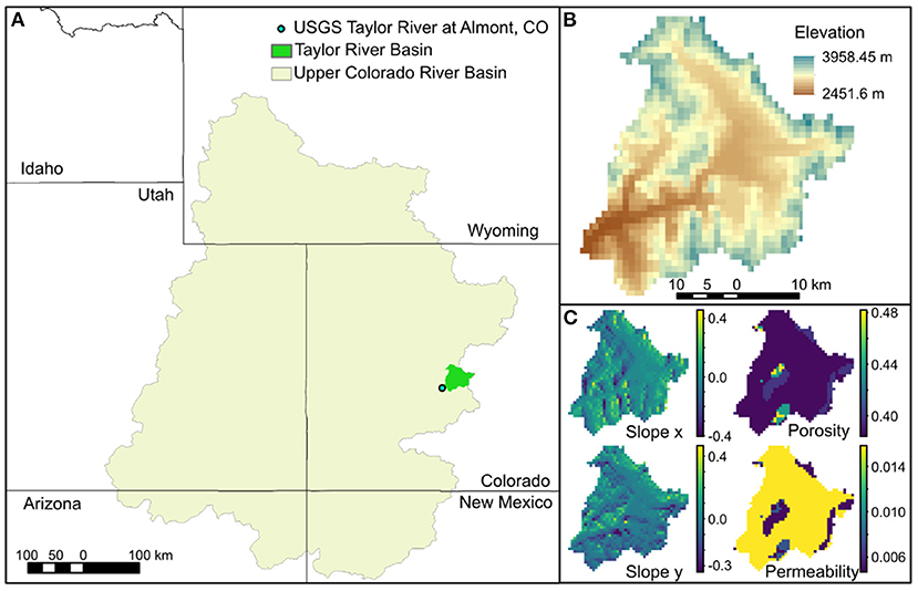
Figure 1. In (A) the mask of the Upper Colorado River Basin and the Taylor river catchment used in this analysis, as well as the USGS gage 09110000 (Taylor River at Almont) used for the definition of the domain. In (B), the elevation map at 1 km resolution (resolution of the analysis), and in (C), the three static inputs used in the training of the machine learning models which are consistent with the corresponding ParFlow-CLM inputs: Slopes in x and y directions, surface porosity, and surface permeability.
2.2. Physics-based model: ParFlow-CLM
To generate the reference simulations, we use the integrated hydrological model ParFlow. It simultaneously solves 3D Richards' equations in the subsurface and the 2D shallow water equation (kinematic wave approximation) for surface flow. It is coupled with the Common Land Model (CLM), which is responsible for simulating the land surface processes (i.e., water and energy balance), as described in Maxwell and Miller (2005) and Kollet and Maxwell (2008): CLM obtains the soil moisture distribution over the top 4 soil layers from ParFlow as well as the hydrological forcing and returns to ParFlow the net infiltration into the soil.
All the required input files, i.e., soil properties, landcover, and meteorological forcing, are a subset of those used for Upper Colorado River Basin ParFlow-CLM simulations in Tran et al. (2020). The boundary conditions are set to no flow for all lateral domain edges as well as the bottom of the domain, while the overland flow is computed on the domain's surface. The spatial resolution of the different inputs and the solver grid is 1 × 1 km, with 5 vertical layers of increasing thickness for a total depth of 102 m. The simulation is run with hourly timesteps for 36 water years, from 1983 to 2018.
In addition to the historical simulations (Historical Forcing, HF), we also generate 12 synthetic drought scenarios. We decrease historical precipitation by a random multiplicative correction factor between 0.5 and 1 (Pscenario = cP*Phistoricalforcing) and increase the historical temperature by an additive factor between 0 and 1° (Tscenario = Thistoricalforcing+cT) for each of the historical water years. These corrections are homogeneous in space and time and are, therefore, the simplest way to have forcing which is still realistic (as intermittency and spatial variability changes are kept consistent with historical observations), but different from what was previously observed. The corrections are designed to mimic a drought climate scenario (scenarios and respective correction factors are indicated in Table 1). All the other meteorological inputs required by ParFlow-CLM (radiation, specific humidity, wind speed, and atmospheric pressure) are kept as in the corresponding historical water year.

Table 1. The first 3 columns summarize the forcing scenarios run with ParFlow-CLM and used for the training and testing of the machine learning models.
ParFlow-CLM is run with all of the forcing scenarios for 10 water years, selected as the driest between 1983 and 2018 (lowest annual precipitation and highest mean temperature, refer to Figure 9). Additionally, the 12 additional forcing scenarios are generated for each of those water years (i.e., 10 water years * 12 scenarios = 120 additional sets of forcing). In addition to the input slopes, permeability, and porosity (Figure 1C), three ParFlow-CLM outputs are utilized here for the training and testing of the ML models: soil infiltration (qflx_infl in ParFlow-CM), vegetation transpiration (qflx_tran_veg in ParFlow-CM), and surface soil moisture. The latter is obtained by multiplying the 2D fields of surface saturation simulated by ParFlow-CLM by the surface porosity (top right in Figure 1C). We choose to consider surface soil moisture as it controls exchanges to the atmosphere, it is very dynamic, and it is comparable to the available product such as remote sensing measurements. For most of the results, unless otherwise specified, only the 10 driest years are considered.
2.3. Convolutional neural networks
We use the simulations introduced in Section 2.2 to train and test two machine learning models designed to predict 2D soil moisture fields. We choose to use Convolutional Neural Network to take advantage of the strong spatial structures in the soil moisture fields and the different variables affecting its distribution. In fact, we choose the inputs to capture the main drivers of soil moisture temporal changes (net infiltration and transpiration) and the spatial variable properties controlling water redistribution both vertically and laterally (surface permeability and porosity, and slopes).
Building upon the model exploration carried out in Maxwell et al. (2021), we select two CNNs: a 2D CNN consisting of 2 Convolution+ReLu layers, each followed by a Max Pooling layer, and two fully connected linear layers (refer to Table A3 in Maxwell et al., 2021), and a 3D CNN which has the same architecture as the 2D model, but an additional Convolution+ReLu first layer (refer to Table A1 in Maxwell et al., 2021).
The inputs for both CNNs are porosity, permeability, slopes and net infiltration, transpiration, and soil moisture. For 3D ParFlow-CLM variables (static variables and soil moisture), the surface layer is considered. All dynamic variables are resampled to daily resolution, by averaging the values in the hours within each day. Furthermore, all inputs are scaled into 0:1 or –1:1 ranges to facilitate training of the CNNs.
The 2D CNN treats all timesteps (i.e., days in the year) as independent and uses the soil moisture field on the following day as the label (left panel in Figure 2). The 3D CNN is built by considering time as the 3rd dimension. The 2D arrays of static inputs, as well as the day-one ParFlow-CLM surface soil moisture (initial conditions), are repeated in the 3rd dimension to match the size of the dynamic inputs, of shape ny, nx, nt (with y being South-North direction, x being West-East direction, and t being time). The label for 3D CNN is the (ny, nx, nt) matrix of soil moisture for the water year. Both these models are trained on 5 water years (1988, 1990, 2015, 2016, and 2018), and 3 different water years (2000, 2012, and 2013) are used for validation and early stopping. When the mean loss (smooth L1 loss) over the last 100 epochs on the validation set is lower than the mean loss over the antecedent 100 epochs, the training is stopped. This is done to avoid over-fitting the machine learning model. Every set-up and model configuration (i.e., model architecture or training data set) is repeated 10–15 times to verify the impact that initialization (initial weights) of the CNNs has on the final results and performances. Unless otherwise stated, individual lines plotting one specific experiment in the results represent the median among the ensemble of initialisations for a given architecture.
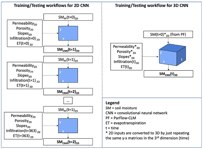
Figure 2. Workflow for the training and testing of the 2D (left) and 3D (right) Convolutional Neural Network. For the 2D architecture at every timestep, the static and dynamic inputs as well as the soil moisture simulated by ParFlow-CLM are fed to the model, while the soil moisture of the next day is provided as the label (or predicted in testing mode). This operation is repeated on all days of the year. For the 3D architecture, the 3rd dimension is time, and all static inputs (including soil moisture at day 0) and dynamic ones are fed to the model, while the label is the 3D moisture field. 2D (static) inputs are repeated for the 3rd (time) dimension.
First, we train both 2D and 3D CNNs with the ParFlow-CLM simulations obtained with historical forcing. This allows us to explore whether these models are capable of reproducing the soil moisture fields as simulated by ParFlow-CLM and compare the 2D and 3D CNNs. Then, we explore the potential of combining physics-based modeling and machine learning in the context of a changing climate by training the CNN either only on historical forcing simulations or both historical forcing and 11 of the forcing scenarios (D1-D11 in Table 1) simulations, and testing on the twelfth scenario (D12).
To compare the performances over the testing year (2002), we use the Root Mean Square Difference (RMSD), the Nash-Sutcliff Efficiency (NSE), and the Kling-Gupta efficiency (KGE, Gupta et al., 2009), computed as follows:
where PF and ML are respectively the soil moisture as simulated by ParFlow-CLM and the machine learning model, μ is the mean, σ the standard deviation, and Cov the covariance.
All these statistics are computed both in space: i.e., the 2D fields of PF and ML are compared at each timestep (i is the spatial index, in x and y); and in time: i.e., the timeseries of PF and ML at every 1km × 1km grid-cell within the catchment are compared (i is the temporal index). The first operation results in a timeseries of these statistical metrics while the latter is summarized in a map (one value for each domain grid-cell).
3. Results
3.1. 2D convolutional neural network
We train the 2D CNN with historical forcing simulations and test it on the water year 2002 (1 Day: blue line in Figure 3A and left column in Figure 3B). Overall the CNN model performs well, with the RMSD typically lower than 0.025, and NSE and KGE higher than 0.9. Inspecting the temporal statistics (Figure 3B, 2D 1 Day), we can see that the trained machine learning model is performing well in most locations. NSE and KGE seem to worsen at the river network, especially in upstream locations (in the North-Western part of the domain, see the mean soil moisture for the water year 2002 in Figure 7 to identify the river network). Surprisingly, the performance of this CNN model is worse than those obtained assuming persistence 1 day to the next, i.e., assuming that the soil moisture does not change (Persistent (t-1) in Figures 3A,B). The explanation for this result is that the soil moisture changes are so small within most timesteps (changes over 1 day), that the CNN model overestimates them, leading to larger RMSD. Proof of this is in the performances during the rainfall events in the later part of the water year, when sharp peaks in net infiltration, mirrored by sharp peaks in soil moisture, lead to better performances of the CNN model than in the persistent case.
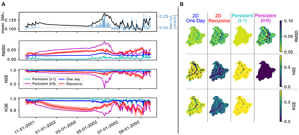
Figure 3. In (A), the timeseries of ParFlow-CLM (PF) domain average in time for the water year 2002 (mean SMPF) and the simulated net infiltration (qflx_infl-qflx_tran_veg ParFlow-CLM variables). Below, the timeseries of Root Mean Square Difference, Nash-Sutcliff Efficiency, and Kling-Gupta Efficiency comparing each day the PF soil moisture field to that of the 2D Convolutional Neural Network (CNN) when predicting 1 day to the next (1 Day) or the entire water year starting from day 0 (Recursive). The semi-transparent bands represent the 0.2–0.8 interquartile ranges among repetition of the same ML configuration (i.e., different initialization). In (B), the temporal statistics comparing the timeseries at each pixel of PF and the 2D CNN in the two configurations, as well as the persistent case in which PF soil moisture is assumed to remain constant either over the entire water year (Persistent, t = 0, meaning that the soil moisture is assumed to remain as of 1st October of the chosen water year) or 1 day to the next (Persistent, t-1).
Models for soil moisture predictions are typically used to simulate over time periods of weeks or months, rather than just the following day. We test the applicability of the CNN model to longer-running simulations. We use the same trained 2D CNN model, but carry out the testing in a different way: instead of using the soil moisture field at t simulated by ParFlow-CLM to make the t+1 prediction, we use the CNN output field of the previous timestep (Recursive). That means that t will be predicted by using the soil moisture field predicted from t−1 (i.e., on the left side of Figure 2, we replace SMPF with SMCNN for t>0). This way, we are only using the soil moisture field from PF on the first day of the year. If we look at the performances in this experiment (Recursive: red lines in Figure 3A and second column in Figure 3B), they expectedly worsen compared to just predicting 1 day to the next. While they still remain reasonably good (RMSD < 0.1), all the statistical measures decline. Furthermore, the sensitivity of the results to the initial conditions increases (refer to semi-transparent regions around the median line in Figure 3A, which corresponds to the 0.2–0.8 quantile band of the trained 2D CNN models). The corresponding persistence case (Persistent (t=0) in Figures 3A,B) is now performing much worse, especially during/after the snowmelt season when soil moisture peaks and then return to drier conditions, more similar to the beginning of the water year. The same is true also looking at the spatial statistics map (Figure 3B), where the RMSD is highest, especially in the Eastern part of the catchment. The NSE is smaller than 0 over the entire catchment and KGE is not available (correlation with a constant cannot be computed).
To further study the performances of the 2D CNN with increasing lead time, we analyse after how many days the 2D CNN outperforms the persistence case. We focus on the latter part of the year, following the peak of domain averaged soil moisture (Figure 4). We compare the RMSD of the 2D CNN and the persistent case as a function of the number of days since the peak soil moisture. The crossover in RMSD occurs after 12 days for the water year 2002 and 7 days for the water year 2017 (other “drought” years not used in training/validation). For wetter years, which the model has not seen in training as the focus was on drier/hotter years, the crossover occurs slightly later, after 20 (water year 1994) and 26 days (water year 2014).
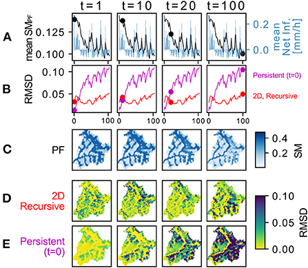
Figure 4. Comparison of soil moisture predictions with the trained 2D CNN and persistence from the peak soil moisture. (A) shows the timeseries of domain average soil moisture as simulated by ParFlow-CLM since the peak soil moisture of Water Year and the corresponding net infiltration (qflx_infl - qflx_tran_veg ParFlow-CLM variables). In (B), the timeseries of Root Mean Squared Differences for the 2D CNN model and the persistent case, in which the 2D soil moisture at the peak is just assumed to remain constant throughout the rest of the year. The markers in (A,B) highlight the time of the snapshot (columns), as reported on top of the figure. In (C), the snapshots of ParFlow-CLM soil moisture fields at the different time steps, and in (D,E), the corresponding RMSD maps for the 2D CNN (2D Recursive) and assuming soil moisture does not change in time (Persistent (t=0), soil moisture is assumed to remain constant as on the day of the peak soil moisture).
3.2. 3D convolutional neural network
The 2D CNN designed here learns the behavior from one timestep to the next and while there is some natural encoding of the temporal behavior in the spatial patterns, this is not enough to persist over long times. Each day, only the static and dynamic inputs at the current time are used to predict the next day's soil moisture. The reasoning behind this choice is that also ParFlow-CLM uses only the current meteorological forcing to simulate each timestep and encodes the model temporal memory in the 3D subsurface states, but because here we are only looking at surface soil moisture we are missing other variables which represent the “memory” of ParFlow-CLM (deeper soil moisture/water pressure). To account for the temporal dimension, we decide to train a 3D CNN, where time is the 3rd dimension. This experiment is comparable to the 2D CNN recursive case, as only soil moisture on the first day is input to the neural network.
The 3D CNN improves model performance compared to the 2D CNN in both space and time (Figure 5). All the statistics considered (RMSD, NSE, and KGE) are better for the 3D CNN model for most of the water year (Figure 5A). Furthermore, the performances are superior also over a larger part of the domain (Figure 5B). The 3D CNN model is performing well over the entire catchment, reproducing the gradual decline in soil moisture during winter, better capturing both the high soil moisture during snowmelt (central column in Figure 6, when 2D CNN underestimates wetness, especially in the North-East), and also the low soil moisture toward the latter part of the water year (right column in Figure 6; while both models seem to overestimate wetness, the overestimation is more evident for the 2D CNNs).
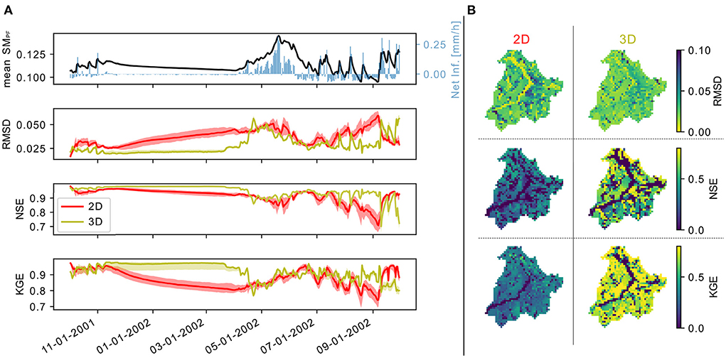
Figure 5. In (A) the timeseries of ParFlow-CLM (PF) domain average in time for water year 2002 (mean SMPF) and the simulated net infiltration (qflx_infl-qflx_tran_veg ParFlow-CLM variables). Below the timeseries of Root Mean Square Difference, Nash-Sutcliff Efficiency, and Kling-Gupta Efficiency comparing the PF mean to that of the 2D Convolutional Neural Network (CNN) (2D) or the 3D CNN (3D). The semi-transparent bands represent the 0.2–0.8 interquantile ranges among repetition of the same ML configuration (i.e., different initialization). In (B) the temporal statistics comparing the timeseries at each pixel of PF and the 2D and 3D CNNs.
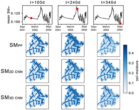
Figure 6. Comparison of soil moisture fields at 3 different timestamps (t=100, 240, 340 d) in Water Year 2002 (day 0 is the 1st of October 2001). On top the timeseries of the ParFlow-CLM soil moisture field average, with a red marker indicating the timestamp, then the fields simulated by ParFlow-CLM, those produced by the 2D trained CNN model, and at the bottom those produced by the 3D trained CNN model.
Over the river network (refer to mean soil moisture as simulated by ParFlow-CLM in Figure 7), the performances drop, mostly due to the fact that ParFlow-CLM surface soil moisture is constant, at saturation, over the entire water year. This is particularly evident looking at the timeseries of ParFlow-CLM and CNN soil moisture for some selected points within the catchment (refer to Location B in Figure 7). As the ParFlow-CLM soil moisture remains stable at its maximum, the NSE and KGE drop to very low (KGE) or very negative (NSE) values. Looking at soil moisture timeseries for some chosen representative locations (Figure 7), it can be seen how the 2D CNN seems to smooth out the soil moisture response, overestimating soil moisture during the drying phase at the beginning of the year and underestimating the snowmelt induced soil moisture peak (consistently with what shown in Figure 6). The 3D CNN seems to match well all parts of the water year soil moisture changes, but anticipate the soil moisture increase (especially at locations A and C in Figure 7). Furthermore, it also introduces a lot of variability (fluctuations around a “constant” value) in the locations where soil moisture is at its maximum (saturation, Location B). The latter period of the water year, following the soil moisture peak, is very well captured, especially by the 3D CNN, with the exception of the river network locations (e.g., Location B), where a decrease in soil moisture is introduced which is not present in ParFlow-CLM simulations. Comparing the timeseries of soil moisture of the CNN models with the long term mean timeseries (computed considering all 36 years, 1983–2018), facilitates the understanding of the behavior of the two models. The 2D CNN model treats every day as completely independent and sees only 1-day timesteps. It, therefore, responds very strongly to forcing (net infiltration in Figure 7). On the other hand, the 3D CNN sees all timesteps within the year and learns much better the seasonal patterns. In other words, the 3D CNN is biased toward the mean and responds less strongly to individual forcing events. This explains the superior performances of the 3D CNN in the snowmelt season. It also explains the earlier peak for some of the locations, where soil moisture responds to positive infiltration with a delay not present in training years, and the more smoothed behavior toward the end of the water year, where the 2D CNN responds better to strong rainfall events.

Figure 7. Soil moisture timeseries at the 4 locations (A, B, C, and D) identified in the map of average Parflow-CLM soil moisture for the water year 2002. These are arbitrary locations selected to show the model behavior at different locations (e.g., B is on the river network, D is upstream, A is further from the river network, and C is next to an upstream contributor). The timeseries of ParFlow-CLM (continuous black line) are compared to the estimates with a 2D convolutional neural network (2D) and a 3D convolutional neural network. The semi-transparent lines represent the different ML models trained (different weight initialization), while the darker lines show the median of those lines for the 2D and 3D models. The corresponding performances are reported in the Table. The dashed line represents the long term mean timeseries of soil moisture simulated by ParFlow-CLM at each location, computed over the 36 years available (i.e., for each day, the mean over the 36 years for that day).
3.3. Forcing scenarios
Finally, we test the potential of combining physics-based modeling and machine learning in the context of a changing climate by looking at the performances when predicting a climate outside the range of that observed in training. We focus on the 3D CNN due to its superior performances but the same results could also be observed also with the 2D CNN model. We compare two sets of 3D CNN models, with the same architecture but trained either only on historical forcing ParFlow-CLM simulations, or also on those with altered forcing (11 scenarios, mimicking drought scenarios by randomly decreasing precipitation and increasing temperature).
Model performances with the additional training scenarios are superior both in time and space (Figure 8). In fact, the RMSD is lower, and NSE and KGE are higher over the entire water year when training not only on historical forcing and the performances are also improved over a large portion of the domain. The 3D CNN model trained only on historical forcing performs worse on the testing scenario used here (D12 in Table 1) rather than on the historical forcing, both for the water year 2002 (comparing the yellow line in Figures 5, 8). This means that indeed when experiencing a climate outside the range of the training data, the performances worsen. The same is not true if the CNN model is also exposed to drought scenario simulations in the training. In fact, the performances are better in the testing even if the specific testing scenario is not used in training (training is done with scenarios D1-D11 and historical forcing).
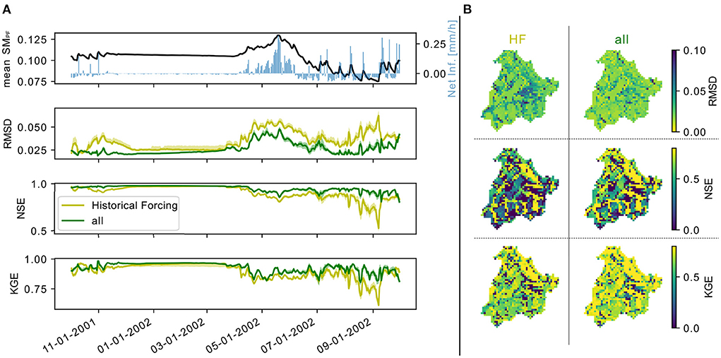
Figure 8. In (A), the timeseries of ParFlow-CLM (PF) domain average in time for the water year 2002 and the testing forcing scenario (mean SMPF) and the simulated net infiltration (qflx_infl-qflx_tran_veg ParFlow-CLM variables). Below, the timeseries of Root Mean Square Difference, Nash-Sutcliff Efficiency, and Kling-Gupta Efficiency comparing the PF mean to that of the 3D Convolutional Neural Network (CNN) trained only on the historical forcing simulations (Historical Forcing, HF) or also on the additional forcing scenarios (all). The semi-transparent bands represent the 0.2-0.8 interquartile ranges among repetitions of the same ML configuration (i.e., different initialization). In (B), the temporal statistics comparing the timeseries at each pixel of PF and the 3D CNN trained just on historical forcing simulations or also on those with additional forcing scenarios.
4. Discussion
In this work, we explore how machine learning and physics-based hydrological modeling can be successfully combined to predict efficiently 2D moisture fields. The former being strongly dependent on the training/input data quality and quantity but extremely computationally efficient makes it very compatible with a physics-based model which is informative but computationally expensive. For the case study presented here, ParFlow-CLM runs one water year simulation in ca. 25 min when using 9 CPUS. We demonstrate how a CNN can be trained by using the simulations generated with ParFlow-CLM and reproducing its soil moisture estimates. Making a 1 water year prediction with the trained ML models takes few seconds on one CPU. As a reference, the performances of a very simple water balance model based on the same inputs as the CNN, are much worse than the ones obtained here with the machine learning models (RMSD>0.2 and negative NSE and KGE).
Having an informative physics-based model, allows us to go beyond past observations and create simulations that are generated using forcing altered to resemble expectations of the future climate. With this training set, the CNN model not only learns how to emulate ParFlow-CLM response to forcing but also how changes in forcing manifest in the soil moisture response. In fact, the model has learned what the effect of an increase in temperature and decrease in precipitation have on soil moisture. The CNN model can then be used to better predict the soil moisture response to climate which has similar properties (in this case, reduced precipitation and increased temperature), but it is different from what was seen in training. This tool can be used to explore many different possible scenarios, in the context of an uncertain future, which would be computationally unfeasible with ParFlow-CLM directly. It is interesting to notice that the two models (trained on just historical forcing or also on the additional forcing scenarios) perform very similarly if tested on a validation year (i.e., water year that has not been used in training) but with historical forcing (refer to Supplementary Figure S2). This confirms that indeed exposing the model to a “different climate” is not simply improving the model because it is trained on more data (5 water years * 11 forcing scenarios = 55 extra water years to train on), but it's also learning the impact of increasing temperature and decreasing precipitation. In the testing scenario (D12) which neither model has seen in training, the superiority of the one that has seen altered forcing is evident.
One of the biggest limitations of this study is the choice of forcing scenarios. These are chosen to reproduce a plausible (intra-annual variability) field of forcing variables with altered statistics (changing the precipitation and temperature homogeneously in space and time). This choice allows for a controlled experiment, where only a small perturbation is applied, but the resulting scenarios are not actually realistic as future climates. More complex changes are expected in the future, with temporally and spatially heterogeneous impacts on precipitation and temperature, but also the other considered meteorological inputs (e.g., Trenberth, 2005). This could be considered in future work, by using weather generators (e.g., Semenov and Barrow, 1997; Kilsby et al., 2007; Peleg et al., 2017), which produce realistic fields of the different meteorological variables, provided (some) statistical properties. Using more realistic future climate scenarios, that are not just homogeneously modified, would probably harden the training of the CNNs to the impact that changing the climate has on soil moisture and require more training simulations with altered forcing.
The same conclusions of the scenarios experiment are also true for wetter or drier water years. The focus here is on droughts and therefore we select drier years (higher mean temperature and lower mean precipitation) between 1983 and 2018. If the trained model is used to predict wetter years, the performances worsen. To show this, while it was not the purpose of the study presented here, we look at the performances of the trained 3D CNN when we predict all 36 water years available (Figure 9, refer to Supplementary Figure S1). While a lot of scattering can be observed the trends are clear across all statistical metrics: the performances worsen with increasing total precipitation and decreasing mean hourly temperature. This confirms once again the importance of the training data quality and specifically whether they are representative (ergodicity). Similar conclusions can be drawn by looking at the comparison of the performances using the 3D CNN or the long term mean (LTM) timeseries (Figure 10). The 3D CNN is outperforming the LTM for drier years (lower yearly precipitation) but is performing worse on wetter ones. Where CNN is really outperforming is on the scenarios, which are much drier than the “average year”. These conclusions are consistent with the out-of-sample testing results in Maxwell et al. (2021). When developing a framework such as the one presented here, it is important not only to ensure that enough training data are generated with the physics-based model, but also that those are tailored to the specific application of interest and intended use.
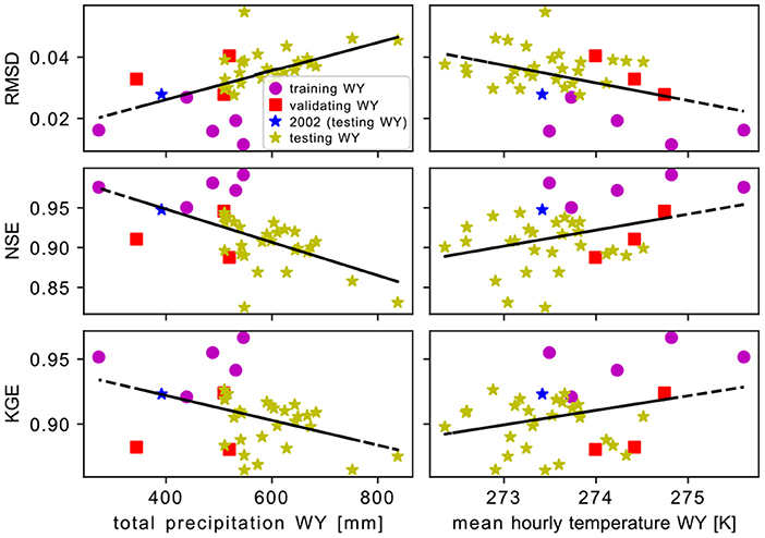
Figure 9. The mean root mean square error (RMSD, first row of plots), Nash-Sutcliffe Efficiency (NSE, middle row of plots), and Klige-Gupta Efficiency (KGE, lower row of plots) as a function of the total precipitation (left column of plots) or the mean hourly temperature (right column of plots) computed for each water year. The color identifies water years used in training, validation, or testing. The water year 2002, used for all the results reported here is marked blue. Black lines represent the trends of a linear fit.
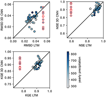
Figure 10. The mean root mean square error (RMSD, first row of plots), Nash-Sutcliffe Efficiency (NSE, middle row of plots), and Klige-Gupta Efficiency (KGE, lower row of plots) as a function of the total precipitation (left column of plots) or the mean hourly temperature (right column of plots) computed for each water year. The color identifies water years used in training, validation, and testing. The water year 2002, used for all the results reported here is marked blue. Black lines represent the trends of a linear fit.
The benefits of the combination of physics based modeling and machine learning have been shown here in the context of a changing climate but they extend to other potential applications which require a large number of simulations such as improving physics based models parametrisation (refer to e.g., Maxwell et al., 2021).
5. Conclusion
In this manuscript, we show how convolutional neural networks can be trained to efficiently predict soil moisture fields as simulated by the physics-based hydrological model ParFlow-CLM. Furthermore, we show how these complementary approaches can be successfully combined to compensate for the computational costs of the physics-based model and the need for tailored training data to properly train a machine learning approach to predict an unprecedented climate. The main findings of this study are:
• Convolutional Neural Networks (CNNs) can be trained and used to predict the soil moisture fields simulated by ParFlow-CLM,
• 3D CNNs, which consider time as the third dimension, outperform 2D CNN both in space in time, better capturing the soil moisture dynamics in space and time, but the 2D CNN reproduced better the soil moisture peaks following strong rainfall events (i.e., rapid soil moisture changes),
• Using the physics-based model to generate additional simulations representative of the expected future changes, can improve the prediction of a “new” forcing scenario (unseen in the training),
• CNNs can predict 2D soil moisture fields very efficiently, within just few seconds for an entire water year (ca. 500 times faster than running ParFlow-CLM),
• The representativeness of the training data is key for the success of the CNNs and ParFlow-CLM simulations should be tailored to the specific application of interest (here drought conditions).
Although future climate scenarios considered in this study are not realistic, the results are proof of how complementary these two approaches are and provide a framework that could be further developed by improving forcing scenarios e.g., with weather generators, and tailoring the training simulations to any application of interest.
Data availability statement
The datasets presented in this study can be found in online repositories. The names of the repository/repositories and accession number(s) can be found below: https://github.com/HydroGEN-pubs/Taylor_CO.git.
Author contributions
EL and RM: conceptualization and formal analysis. EL: data curation, visualization, and writing—original draft. LC, RM, and EL: funding acquisition. EL, HT, RBH, LD, PM, LC, and RM: investigation and validation. EL, HT, RBH, LD, LB, PM, LC, and RM: methodology. LC and RM: project administration. EL and VB: software. LC, PM, and RM: supervision. RBH, LC, and RM: writing—review and editing. All authors contributed to the article and approved the submitted version.
Funding
This research was funded by the US National Science Foundation Convergence Accelerator Program, Grant No. CA-2040542 and the Swiss National Science Foundation, Grant No. P500PN_202745.
Conflict of interest
The authors declare that the research was conducted in the absence of any commercial or financial relationships that could be construed as a potential conflict of interest.
Publisher's note
All claims expressed in this article are solely those of the authors and do not necessarily represent those of their affiliated organizations, or those of the publisher, the editors and the reviewers. Any product that may be evaluated in this article, or claim that may be made by its manufacturer, is not guaranteed or endorsed by the publisher.
Supplementary material
The Supplementary Material for this article can be found online at: https://www.frontiersin.org/articles/10.3389/frwa.2022.927113/full#supplementary-material
References
Bierkens, M. F. P., Bell, V. A., Burek, P., Chaney, N., Condon, L. E., David, C. H., et al. (2015). Hyper-resolution global hydrological modelling: what is next? Hydrol. Process 29, 310–320. doi: 10.1002/hyp.10391
Bogaard, T. A., and Greco, R. (2018). Invited perspectives: Hydrological perspectives on precipitation intensity-duration thresholds for landslide initiation: proposing hydro-meteorological thresholds. Natural Hazards Earth Syst. Sci. 18, 31–39. doi: 10.5194/nhess-18-31-2018
Bolten, J. D., Crow, W. T., Jackson, T. J., Zhan, X., and Reynolds, C. A. (2010). Evaluating the utility of remotely sensed soil moisture retrievals for operational agricultural drought monitoring. IEEE J. Select. Top. Appl. Earth Observat. Remote Sens. 3, 57–66. doi: 10.1109/JSTARS.2009.2037163
Chen, L., Cao, Y., Ma, L., and Zhang, J. (2020). A deep learning-based methodology for precipitation nowcasting with radar. Earth Space Sci. 7, e2019EA000812. doi: 10.1029/2019EA000812
Dobriyal, P., Qureshi, A., Badola, R., and Hussain, S. A. (2012). A review of the methods available for estimating soil moisture and its implications for water resource management. J. Hydrol. 458–459, 110–117. doi: 10.1016/j.jhydrol.2012.06.021
ElSaadani, M., Habib, E., Abdelhameed, A. M., and Bayoumi, M. (2021). Assessment of a spatiotemporal deep learning approach for soil moisture prediction and filling the gaps in between soil moisture observations. Front. Artif. Intell. 4, 636234. doi: 10.3389/frai.2021.636234
Gupta, H. V., Kling, H., Yilmaz, K. K., and Martinez, G. F. (2009). Decomposition of the mean squared error and nse performance criteria: Implications for improving hydrological modelling. J. Hydrol. 377, 80–91. doi: 10.1016/j.jhydrol.2009.08.003
IPCC (2021). IPCC Press Release, 9 Aug. 2021. IPCC Press Conference. Available online at: https://www.ipcc.ch/site/assets/uploads/2021/08/IPCC_WGI-AR6-Press-Release_en.pdf (accessed 22 March, 2022).
Kilsby, C., Jones, P., Burton, A., Ford, A., Fowler, H., Harpham, C., et al. (2007). A daily weather generator for use in climate change studies. Environ. Model. Software 22, 1705–1719. doi: 10.1016/j.envsoft.2007.02.005
Kollet S. J. Maxwell R. M. (2008), Capturing the influence of groundwater dynamics on land surface processes using an integrated, distributed watershed model. Water Resour. Res. 44, W02402. 10.1029/2007WR006004
Kratzert, F., Klotz, D., Shalev, G., Klambauer, G., Hochreiter, S., and Nearing, G. (2019). Towards learning universal, regional, and local hydrological behaviors via machine learning applied to large-sample datasets. Hydrol. Earth Syst. Sci. 23, 5089–5110. doi: 10.5194/hess-23-5089-2019
Kuffour, B. N. O., Engdahl, N. B., Woodward, C. S., Condon, L. E., Kollet, S., and Maxwell, R. M. (2019). Simulating coupled surface-subsurface flows with ParFlow v3.5.0: capabilities, applications, and ongoing development of an open-source, massively parallel, integrated hydrologic model. Geoscientific Model Dev. Discuss. 2019, 1–66. doi: 10.5194/gmd-2019-190
Kurtz, W., He, G., Kollet, S. J., Maxwell, R. M., Vereecken, H., and Hendricks Franssen, H.-J. (2016). TerrSysMP-PDAF (version 1.0): a modular high-performance data assimilation framework for an integrated land surface-subsurface model. Geoscientific Model Dev. 9, 1341–1360. doi: 10.5194/gmd-9-1341-2016
Lange, H., and Sippel, S. (2020). “Machine learning applications in hydrology,” in Forest-Water Interactions (Cham: Springer International Publishing), 233–257.
Leonarduzzi, E., McArdell, B. W., and Molnar, P. (2021). Rainfall-induced shallow landslides and soil wetness: comparison of physically based and probabilistic predictions. Hydrol. Earth Syst. Sci. 25, 5937–5950. doi: 10.5194/hess-25-5937-2021
Martínez-Fernández, J., González-Zamora, A., Sánchez, N., Gumuzzio, A., and Herrero-Jiménez, C. M. (2016). Satellite soil moisture for agricultural drought monitoring: assessment of the smos derived soil water deficit index. Remote Sens. Environ. 177, 277–286. doi: 10.1016/j.rse.2016.02.064
Massari, C., Brocca, L., Barbetta, S., Papathanasiou, C., Mimikou, M., and Moramarco, T. (2014). Using globally available soil moisture indicators for flood modelling in mediterranean catchments. Hydrol. Earth Syst. Sci. 18, 839–853. doi: 10.5194/hess-18-839-2014
Maxwell, R., Condon, L., and Melchior, P. (2021). A physics-informed, machine learning emulator of a 2d surface water model: What temporal networks and simulation-based inference can help us learn about hydrologic processes. Water 13, 3633. doi: 10.3390/w13243633
Maxwell, R. M., Condon, L. E., and Kollet, S. J. (2015). A high-resolution simulation of groundwater and surface water over most of the continental us with the integrated hydrologic model parflow v3. Geoscientific Model Dev. 8, 923–937. doi: 10.5194/gmd-8-923-2015
Maxwell, R. M., and Miller, N. L. (2005). Development of a coupled land surface and groundwater model. J. Hydrometeorol. 6, 233–247. doi: 10.1175/JHM422.1
Merz, B., and Plate, E. J. (1997). An analysis of the effects of spatial variability of soil and soil moisture on runoff. Water Resour. Res. 33, 2909–2922. doi: 10.1029/97WR02204
Mirus, B. B., Morphew, M. D., and Smith, J. B. (2018). Developing hydro-meteorological thresholds for shallow landslide initiation and early warning. Water 10, 1274. doi: 10.3390/w10091274
Narasimhan, B., and Srinivasan, R. (2005). Development and evaluation of soil moisture deficit index (smdi) and evapotranspiration deficit index (etdi) for agricultural drought monitoring. Agric. Forest Meteorol. 133, 69–88. doi: 10.1016/j.agrformet.2005.07.012
Norbiato, D., Borga, M., Degli Esposti, S., Gaume, E., and Anquetin, S. (2008). Flash flood warning based on rainfall thresholds and soil moisture conditions: an assessment for gauged and ungauged basins. J. Hydrol. 362, 274–290. doi: 10.1016/j.jhydrol.2008.08.023
Ochsner, T. E., Cosh, M. H., Cuenca, R. H., Dorigo, W. A., Draper, C. S., Hagimoto, Y., et al. (2013). State of the art in large-scale soil moisture monitoring. Soil Sci. Soc. Am. J. 77, 1888–1919. doi: 10.2136/sssaj2013.03.0093
O'Neill, M. M. F., Tijerina, D. T., Condon, L. E., and Maxwell, R. M. (2021). Assessment of the parflow-clm conus 1.0 integrated hydrologic model: evaluation of hyper-resolution water balance components across the contiguous united states. Geoscientific Model Dev. 14, 7223–7254. doi: 10.5194/gmd-14-7223-2021
Pauwels, V. R. N., Hoeben, R., Verhoest, N. E. C., Ëois, P., and De Troch (2001). The importance of the spatial patterns of remotely sensed soil moisture in the improvement of discharge predictions for small-scale basins through data assimilation. J. Hydrol. 251, 88–102. doi: 10.1016/S0022-1694(01)00440-1
Peleg, N., Fatichi, S., Paschalis, A., Molnar, P., and Burlando, P. (2017). An advanced stochastic weather generator for simulating 2-d high-resolution climate variables. J. Adv. Model. Earth Syst. 9, 1595–1627. doi: 10.1002/2016MS000854
Semenov, M. A., and Barrow, E. M. (1997). Use of a stochastic weather generator in the development of climate change scenarios. Clim. Change 35, 397–414. doi: 10.1023/A:1005342632279
Seneviratne, S. I., Corti, T., Davin, E. L., Hirschi, M., Jaeger, E. B., Lehner, I., et al. (2010). Investigating soil moisture-climate interactions in a changing climate: a review. Earth Sci. Rev. 99, 125–161. doi: 10.1016/j.earscirev.2010.02.004
Sharma, P. K., Kumar, D., Srivastava, H. S., and Patel, P. (2018). Assessment of different methods for soil moisture estimation: a review. J. Remote Sens. GIS 9, 57–73. doi: 10.37591/.v9i1.105
Shen, C., Chen, X., and Laloy, E. (2021). Editorial: Broadening the use of machine learning in hydrology. Front. Water 3, 681023. doi: 10.3389/frwa.2021.681023
Shi, X., Chen, Z., Wang, H., Yeung, D. Y., Wong, W. K., and Woo, W. C. (2008). “Convolutional LSTM network: A machine learning approach for precipitation nowcasting,” in Proceedings of the 28th International Conference on Neural Information Processing Systems (Montreal, QC), 802–810.
Su, A., Li, H., Cui, L., and Chen, Y. (2020). A convection nowcasting method based on machine learning. Adv. Meteorol. 2020, 5124274. doi: 10.1155/2020/5124274
Tran, H., Leonarduzzi, E., De la Fuente, L., Hull, R. B., Bansal, V., Chennault, C., et al. (2021). Development of a deep learning emulator for a distributed groundwater-surface water model: Parflow-ml. Water 13, 3393. doi: 10.3390/w13233393
Tran, H., Zhang, J., Cohard, J.-M., Condon, L. E., and Maxwell, R. M. (2020). Simulating groundwater-streamflow connections in the upper colorado river basin. Groundwater 58, 392–405. doi: 10.1111/gwat.13000
Trenberth, K. E. (2005). “The impact of climate change and variability on heavy precipitation, floods, and droughts,” in Encyclopedia of Hydrological Sciences, ed M. G. Anderson (Hoboken, NJ: Wiley). doi: 10.1002/0470848944.hsa211
Keywords: machine learning, physics-based hydrological model, ParFlow-CLM, 2D soil moisture field, convolutional neural networks, meteorological forcing scenarios
Citation: Leonarduzzi E, Tran H, Bansal V, Hull RB, De la Fuente L, Bearup LA, Melchior P, Condon LE and Maxwell RM (2022) Training machine learning with physics-based simulations to predict 2D soil moisture fields in a changing climate. Front. Water 4:927113. doi: 10.3389/frwa.2022.927113
Received: 23 April 2022; Accepted: 15 September 2022;
Published: 11 October 2022.
Edited by:
Tianjie Zhao, Aerospace Information Research Institute (CAS), ChinaReviewed by:
Shervan Gharari, University of Saskatchewan, CanadaJames Gilbert, University of California, Santa Cruz, United States
Copyright © 2022 Leonarduzzi, Tran, Bansal, Hull, De la Fuente, Bearup, Melchior, Condon and Maxwell. This is an open-access article distributed under the terms of the Creative Commons Attribution License (CC BY). The use, distribution or reproduction in other forums is permitted, provided the original author(s) and the copyright owner(s) are credited and that the original publication in this journal is cited, in accordance with accepted academic practice. No use, distribution or reproduction is permitted which does not comply with these terms.
*Correspondence: Elena Leonarduzzi, bGVvbmFyZHV6emlAcHJpbmNldG9uLmVkdQ==