 Sam Anderson
 Valentina Radić
- Department of Earth, Ocean, and Atmospheric Sciences, University of British Columbia, Vancouver, BC, Canada
The interpretation of deep learning (DL) hydrological models is a key challenge in data-driven modeling of streamflow, as the DL models are often seen as “black box” models despite often outperforming process-based models in streamflow prediction. Here we explore the interpretability of a convolutional long short-term memory network (CNN-LSTM) previously trained to successfully predict streamflow at 226 stream gauge stations across southwestern Canada. To this end, we develop a set of sensitivity experiments to characterize how the CNN-LSTM model learns to map spatiotemporal fields of temperature and precipitation to streamflow across three streamflow regimes (glacial, nival, and pluvial) in the region, and we uncover key spatiotemporal patterns of model learning. The results reveal that the model has learned basic physically-consistent principles behind runoff generation for each streamflow regime, without being given any information other than temperature, precipitation, and streamflow data. In particular, during periods of dynamic streamflow, the model is more sensitive to perturbations within/nearby the basin where streamflow is being modeled, than to perturbations far away from the basins. The sensitivity of modeled streamflow to the magnitude and timing of the perturbations, as well as the sensitivity of day-to-day increases in streamflow to daily weather anomalies, are found to be specific for each streamflow regime. For example, during summer months in the glacial regime, modeled daily streamflow is increasingly generated by warm daily temperature anomalies in basins with a larger fraction of glacier coverage. This model's learning of “glacier runoff” contributions to streamflow, without any explicit information given about glacier coverage, is enabled by a set of cell states that learned to strongly map temperature to streamflow only in glacierized basins in summer. Our results demonstrate that the model's decision making, when mapping temperature and precipitation to streamflow, is consistent with a basic physical understanding of the system.
Introduction
The success of machine learning (ML) for hydrological modeling, and in particular, the unprecedented skill of deep learning (DL) models for streamflow prediction, has emphasized the value of data-driven models for streamflow prediction (e.g., Kratzert et al., 2018; Shen, 2018; Shen et al., 2018). Studies that bench-marked ML models against both calibrated conceptual models and process-based models have agreed that ML models typically perform better (e.g., Hsu et al., 1995; Abramowitz, 2005; Best et al., 2015; Nearing et al., 2016). However, despite the skill of ML (Zealand et al., 1999; Maier and Dandy, 2000; Maier et al., 2010), and in particular DL for streamflow prediction (Kratzert et al., 2019c; Anderson and Radić, 2022), there is a reservation for using these models in the hydrological community in part due to challenges surrounding data-driven model interpretability (Nearing et al., 2021). Since ML and DL models are often seen as black-box models, their accurate predictions of streamflow have not led to their widespread acceptance despite the growing availability of big data in hydrology. Translating the information learned by DL models into human-interpretable information presents a middle ground for process-based and data-based modeling communities to meet with shared concerns over how models work, how physics is represented, and why models make certain decisions.
Deep machine learning models have been applied across a wide range of hydrological modeling tasks (e.g., Fang et al., 2017; Shi et al., 2017; Bowes et al., 2019), and are attractive due to the existence of architectures that are explicitly designed to learn from spatially discretized information [e.g., convolutional neural networks (CNNs); LeCun et al., 1990] and sequential information (e.g., recurrent neural networks; Rumelhart et al., 1985). Long short-term memory (LSTM) networks are a class of recurrent neural network and are designed to learn from sequential information with dependencies at both long and short timescales (Hochreiter and Schmidhuber, 1997). Together, CNNs and LSTMs can be combined to facilitate the learning of spatiotemporal information, such as for video description (e.g., Donahue et al., 2017). LSTMs in particular have been widely applied for rainfall-runoff modeling tasks (Hu et al., 2018; Le et al., 2019; Sudriani et al., 2019), and recent studies in hydrology have applied LSTMs for streamflow prediction at hundreds of basins at daily timescales (Kratzert et al., 2018, 2019c), at hourly timescales (Gauch et al., 2021), at ungauged basins (Kratzert et al., 2019b), and for extreme events (Frame et al., 2021). Variants of the LSTM have been developed, for example: an entity-aware LSTM (EA-LSTM) that includes static basin characteristics as input in addition to time-varying meteorological forcing (Kratzert et al., 2019c); a sequence-to-sequence LSTM encoder-decoder model for forecasting hourly streamflow over 24 h lead times (Xiang et al., 2020); an LSTM with data integration to incorporate static characteristics and recent streamflow for daily streamflow forecasting (Feng et al., 2020); a mass-conserving LSTM (MC-LSTM) that enforces conservation of mass through the model formulations (Hoedt et al., 2021); an LSTM that combines meteorological forcing and outputs from global hydrological models to improve flood simulations (Yang et al., 2019); and a convolutional-LSTM (CNN-LSTM) that encodes spatially discretized meteorological forcing (Anderson and Radić, 2022). The wide range of LSTM models and variants have been developed with the goal of understanding how to better incorporate available data (e.g., static characteristics, recent observations, hydrological model outputs, spatially discretized information) into differently structured model architectures (e.g., sequence-to-sequence, CNN-LSTM).
Despite the many successes in terms of predictive ability, model interpretability has been an almost ubiquitous challenge across ML and DL modeling approaches. To gain confidence in ML and DL beyond their use as “black box” models, it would be helpful to understand how and why models make decisions, and if these decisions are consistent with known physics. Adherence to physical laws can be encouraged during model training. For example, penalties against non-physical results can be leveraged through the inclusion of a regularization term in the loss function that is large when mass, energy, or momentum is not conserved (e.g., Karpatne et al., 2017; Jia et al., 2019). Alternatively, physical laws can be enforced or encouraged through using physics-informed architectures, such as those that necessarily conserve mass (Hoedt et al., 2021) or ensure physical consistency (Daw et al., 2020). Otherwise, models can be trained without any information on the constraining physical laws, and physical consistency is investigated after model training. In all cases, insights into the models' learning can come from probing the model with various types of diagnostic tools (McGovern et al., 2019). Many of these tools are different types of sensitivity analyses that seek to understand and visualize how the model outputs are linked to and influenced by the model inputs (Razavi et al., 2021). Examples include occlusion, which masks small areas of the input to determine importance of local structure to model decision making (Zeiler and Fergus, 2014); layerwise relevance propagation, which determines the importance of input features for any given output by backpropagating through the network from a single output neuron (Bach et al., 2015); saliency maps, which calculate how an output prediction changes with small changes of each input value (Simonyan et al., 2014); backward optimization, which calculates input examples that maximally activate particular output neurons (Olah et al., 2017); class activation mapping, which uses deep convolutional feature maps to calculate input regions that are most important for classification (Selvaraju et al., 2020); shapely additive explanations (SHAP), which quantifies feature importance as the contribution of each feature to a prediction (Lundberg and Lee, 2017); and local interpretable model-agnostic explanations (LIME), which locally approximates a more complex model with a simpler and interpretable (e.g., linear) model around a prediction (Ribeiro et al., 2016). While there are a growing number of applications of these techniques in the geosciences more broadly (e.g., Gagne et al., 2019; Toms et al., 2020; Mayer and Barnes, 2021), fewer interpretability studies exist in hydrology.
Other interpretability tools include those that seek to understand internal model states by analysis of information contained in embedding or hidden layers of the neural network (Karpathy et al., 2015; Wang et al., 2017; Bianchi et al., 2020). The analysis of cell states in the hidden layers of LSTM models is found to be particularly useful when it comes to identifying human-interpretable information. By investigating the hidden layers, Kratzert et al. (2019a) showed that an LSTM trained for streamflow prediction contained internal states that were linked to snow cover and soil water storage. While no direct information about snow or soil variables was given a priori to the model, it has learned hydrologically relevant and interpretable behavior about these unobserved variables. The same study also demonstrated that the LSTM model determined that a longer time history is needed for making predictions in a snowmelt dominated basin relative to a rainfall dominated basin, consistent with the understanding that the process of snowmelt depends on a longer time history (e.g., runoff from the accumulation and ablation of a snowpack vs. daily scale runoff from rainfall). Another study, which used CNN-LSTMs to map spatiotemporal series of meteorological variables to regional streamflow, also identified the model's ability to learn different runoff-generation mechanisms across the region (Anderson and Radić, 2022). In particular, for glacierized basins, the models automatically learned that late summer streamflow responses are linked to the extent of glacier cover per basin, without any a priori knowledge about the glacier cover. Wunsch et al. (2022) used a CNN-LSTM for predicting streamflow in karst spring systems and found that the model automatically learned that areas of the input precipitation fields that are within the basin are most important for the model's decision making, suggesting that CNN-LSTMs may be useful for catchment localization when the basin outlines are not known. While these and other methods are emerging to interpret the spatiotemporal patterns or predictions made by hydrological ML models (e.g., Fleming et al., 2021a,b), there remains an opportunity to better understand the details of ML and DL hydrological model decision making.
The main goal of this study is to demonstrate that a DL model is able to learn some of the key runoff-generating mechanisms across different streamflow regimes, while driving the model only with temperature and precipitation data as input. To do so we will use the previously developed and trained CNN-LSTM model (Anderson and Radić, 2022) for streamflow simulations at 226 stream gauge stations across southwestern Canada. The model, forced only by gridded temperature and precipitation data, is shown to successfully simulate observed daily streamflow between 1980 and 2015 (Anderson and Radić, 2022). Streamflow across the region is primarily driven by snowmelt, glacier melt, rainfall, and groundwater flow, leading to a range of nival, pluvial, glacial, and intermediate streamflow regimes (Eaton and Moore, 2010). This variety of runoff-generating mechanisms is ideal for exploring DL model interpretability. To do so, we design a set of experiments to probe the model's ability in learning runoff-generating mechanisms for different streamflow regimes. The experiments are set around basic hydrological concepts of the response of streamflow in space, time, and across streamflow regimes, to perturbations in the forcing temperature and precipitation.
We investigate the model's learning of runoff-generating mechanisms by first partitioning the stream gauge stations into clusters whose stations share a similar streamflow regime. For our first set of experiments, we ask the following questions for each streamflow regime: How does the modeled streamflow respond to spatially varying perturbations in input data, and how does this response vary over a year? How does the importance of the driving input variables (temperature and precipitation) vary over a year? What weather conditions, set by the input variables, cause the model to predict substantial increases in streamflow? Our second set of experiments aims at probing the inner states of the LSTM component of the model to investigate how physically interpretable cell states can be identified. Here we focus on differences between glacier-fed vs. non-glacier-fed river regimes to identify cell states that represent glacier contributions to streamflow. The study is structured in the following way: Background and Materials reviews the study region and data used, Methods describes the details of the interpretability experiments, and Results, Discussion, and Summary and Conclusion present and interpret our findings.
Background and Materials
Study Region
The study region is southwestern Canada in the provinces of British Columbia and Alberta, south of 56°N and west of 110°W (Figure 1, Supplementary Figure 1). Streamflow in low elevation basins along the west coast is predominantly pluvial, where most precipitation occurs in fall and winter and most often falls as rain. However, temperatures decrease further inland and at higher elevation, and so intermediate pluvial-nival regimes exist in some coastal basins where high elevation areas are cold enough in winter to accumulate a seasonal snowpack, leading to a spring freshet. Predominantly nival regimes exist through much of the rest of the study region, where colder winter temperatures facilitate the accumulation of a seasonal snowpack (Moore et al., 2010). West of the Rocky Mountains in British Columbia, most precipitation occurs in fall and winter, leading to some runoff before temperatures cool below freezing followed by the accumulation of a substantial snowpack. The eastern slopes of the Rocky Mountains experience substantial snowfall in winter, but much of the region east of the Rocky Mountains in Alberta experiences comparably dry winters due to the rain shadow of the Rocky Mountains and the influence of cold and dry Arctic air. Most precipitation in these areas falls as rain during spring or summer, leading to rainfall-driven streamflow after the freshet has ended in spring.
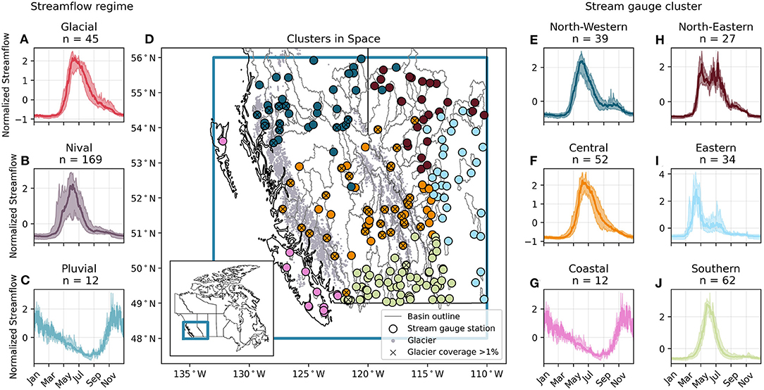
Figure 1. Map of the study region, and hydrographs of streamflow regimes and sub-regional clusters. (A–C) The mean seasonal streamflow patterns of each streamflow regime (solid line), with one standard deviation range (shaded area) derived from all stream gauge stations in the given regime. (D) The basin outlines, and stream gauge locations that are colored according to the geographically constrained seasonal streamflow clusters. Gray dots show the locations of glaciers taken from RGI V6.0. (E–J) The mean seasonal streamflow patterns of each geographically constrained cluster of stream gauges (solid line), with one standard deviation range (shaded area) derived from all stream gauge stations in the given cluster. Note that all stations of the glacial regime (i.e., with >1% glacier coverage) are marked with an “x.” The nival regime is made up of all stations with <1% glacier coverage located in the north-western, central, southern, eastern, and north-eastern clusters. The pluvial regime includes all stations from the coastal cluster.
Thousands of glaciers exist throughout the study region in high alpine areas (Figure 1), and glacier meltwater primarily contributes to streamflow in these basins after the seasonal snowpack has melted. Highly glaciated basins experience a delayed freshet as compared to pluvial basins, with peak flows typically occurring in late summer. Additionally, annual variability of glacier runoff counteracts annual variability of precipitation, where excess melt partially compensates for a lack of precipitation in hot and dry summers, but reduced melt partially counteracts an excess of rain in cool and wet summers (Meier and Tangborn, 1961; Fountain and Tangborn, 1985). The strength of the expression of glacier runoff in streamflow increases non-linearly with glacier coverage (e.g., Stahl and Moore, 2006), leading to complex spatiotemporal patterns of glacier runoff in streamflow throughout the study region (Anderson and Radić, 2020).
Data
A detailed description of the data selection process for both input weather data and output streamflow data can be found in Anderson and Radić (2022); here, we summarize the data used to train, validate, and test the developed CNN-LSTM models. The CNN-LSTM models are forced by spatiotemporal fields of maximum temperature (Tmax(x, y, t)), minimum temperature (Tmin(x, y, t)), and precipitation (P(x, y, t)), all extracted from ERA5 reanalysis from the European Center for Medium-Range Weather Forecasts (ECMWF; Hersbach et al., 2020). Daily fields at 0.75° × 0.75° spatial resolution are aggregated from 1979 to 2015. Both temperature and precipitation have been found to be well-represented in the study region by previous versions of ERA climate reanalysis (Odon et al., 2018, 2019). We access daily streamflow data from Environment and Climate Change Canada's Historical Hydrometric Data (HYDAT) website, which provides historical daily streamflow data (in [m3/s]) at thousands of stations throughout Canada (Environment Climate Change Canada, 2018). We only consider stream gauge stations that are classified as natural (without upstream regulating features) and that have sufficient data during the period 1979–2015, which include the time windows for training, validation, and testing of the CNN-LSTM models. In total, 226 stream gauge stations were used, with station names and numbers listed in the Supplementary Table 1 in Anderson and Radić (2022). The same 226 stations are used in this study.
The 226 stations are clustered into geographically constrained streamflow regimes to define groups of neighboring basins that share similar seasonal hydrographs. This grouping is necessary for our investigation of the model's interpretability. Agglomerative hierarchical clustering with Ward's method (Hastie et al., 2009) is used to cluster stream gauge stations by their seasonal streamflow, latitude, and longitude. In total we identify six clusters whose mean seasonal streamflow patterns, i.e., seasonal streamflow averaged over the stations belonging to each cluster, reveal a range of streamflow regimes throughout the study region (Figures 1A–H). We name the clusters according to their geographical location in the region. The “coastal” cluster exemplifies a pluvial regime where flows are primarily driven by rainfall between October through April, with a minor spring freshet due to snowmelt in the highest elevation areas of some of the basins. The “southern” cluster is predominantly nival, having a spring freshet and little rainfall driven runoff outside of this period. The “eastern,” “north-eastern,” and “north-western” clusters demonstrate both a pronounced spring freshet and a secondary seasonal streamflow peak from rainfall in spring, summer, or fall. The “central” cluster demonstrates a clear spring freshet, but unlike the southern cluster, streamflow decreases more slowly over the course of the summer due to contributions from glacier runoff in some of the basins in the cluster.
We also group stations by streamflow regime (glacial, nival, or pluvial) in addition to the six geographically constrained sub-regional clusters. While this grouping is relatively simple, it aids the interpretability analysis of the CNN-LSTM model. We consider all stations with >1% glacier coverage in their watersheds to be of a glacial regime. We consider stations with a spring freshet and <1% glacier coverage to be of a predominantly nival regime (e.g., all central, southern, eastern, north-eastern, and north-western stations with <1% glacier coverage). Finally, we consider coastal stations dominated by rainfall-driven winter flows to be pluvial.
We use glacier areas and locations from the Randolph Glacier Inventory Version 6.0 to characterize the extent of glaciation in each basin (RGI Consortium, 2017). We access basin outlines for the stream gauge stations in the study region from the Water Survey of Canada (Environment Climate Change Canada, 2016). For each basin, we sum the total area of glaciers within the basin outlines. We divide the total per-basin glacier area by the total basin area to determine the per-basin glacier coverage, G. When G = 0 there are no glaciers in the basin, and when G = 1 the entire basin is glaciated. Across the study region, G ranges from 0 to 0.59, with mean of 0.01 (Supplementary Table A1).
Methods
In this section we briefly describe the CNN-LSTM model and introduce the sensitivity experiments used for interpreting the model's learning. By “interpreting the model's learning” we mean assessing how well the results from these experiments resemble those expected from a conceptual understanding of the hydrological processes (Figure 2). We assess the streamflow response to perturbations in temperature and precipitation only, neglecting further hydrological complexity. The sensitivity experiments address the model's learning of the following basic concepts:
(1) Spatial sensitivity to climate forcing: Climate forcing (temperature and precipitation fields) within a watershed where streamflow is being modeled is a more relevant driver of streamflow than climate forcing outside the watershed.
(2) Regime-specific importance of input variables: The sensitivity of streamflow to the magnitude and timing of perturbations in temperature and precipitation is streamflow-regime specific (Figure 2). In the pluvial regime, streamflow is primarily sensitive to precipitation if temperatures are above freezing. In the glacial and nival regimes, streamflow is insensitive to temperature and precipitation perturbations during winter when sub-freezing temperatures suppress runoff generation. Then, streamflow is highly sensitive to temperature and precipitation perturbations during the spring freshet when small variations in forcing can cause large variations in streamflow. In the nival regime, summer streamflow is more sensitive to precipitation once the seasonal snowpack has melted since rainfall drives runoff; in contrast, in the glacial regime, summer streamflow is sensitive to temperature since glacier melt drives runoff.
(3) Regime-specific sensitivity to anomalous weather conditions: The daily weather anomalies (e.g., wetter or drier than normal, warmer or colder than normal) that drive substantial day-to-day increases in streamflow are also streamflow-regime specific (Figure 2). Warm daily anomalies drive substantial increases in runoff during periods when streamflow is driven by melt (e.g., nival and glacial basins in spring, glacial basins in summer), while wet daily anomalies drive substantial increases in runoff during periods when streamflow is driven by rain (e.g., throughout the year in pluvial basins, during summer in nival basins). In glacial basins, the sensitivity to warm daily anomalies in summer is expected to increase with the glacierized-area fraction per basin because the glacier-melt contribution to streamflow increases with the increase of glacierized-area fraction (Jansson et al., 2003; Frans et al., 2016).
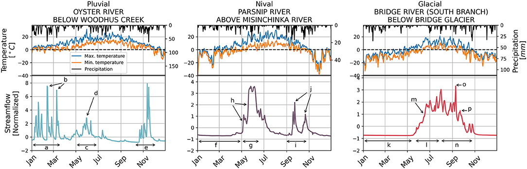
Figure 2. Examples of streamflow, temperature, and precipitation for pluvial, nival, and glacial rivers. Maximum temperature, minimum temperature, and precipitation are taken from ERA5 data at the location of each stream gauge. For the pluvial basin (left panels): (a) Winter pluvial flows are primarily driven by rainfall, but colder temperatures may occur at higher elevation portions of the basin and some precipitation may be stored as snow. (b) Large streamflow events are preceded by precipitation. (c) Spring and early summer pluvial flows may be driven by a small freshet from high elevation snow melt, during which (d) streamflow events can follow dry but warm conditions. (e) Fall pluvial flows are driven by rain and follow precipitation events. For the nival basin (middle panels): (f) Winter and early spring nival flows are suppressed due to below-freezing temperatures. (g) Spring nival flows are driven by snowmelt, and (h) large increases in streamflow follow warm temperatures. (i) Fall nival flows are driven by rainfall, and (j) streamflow events follow precipitation. For the glacial basin (right panels): (k) Winter and early spring glacial flows are suppressed due to below-freezing temperatures. (l) Spring glacial flows are driven primarily by snowmelt, and (m) when warm temperatures drive streamflow. (n) After the snowpack has melted in summer and fall, glacial flows are driven by both rainfall and glacier melt, and streamflow events follow (o) precipitation or (p) warm temperatures.
In addition, we present a method for investigating the model's ability to learn glacier-runoff contributions to streamflow, assuming that this contributor can be represented by a set of cell states in the LSTM component of the model. To detect these ‘glacier-runoff' cell states, we analyze the links between cell states and glacierized-area fraction per basin. If this link is found and it is a strong one, we look for those cell states whose seasonal pattern resembles a conceptual seasonal pattern of glacier runoff.
Model
We use the trained CNN-LSTM models as developed and described in detail in Anderson and Radić (2022). Here we provide a summary of the model architecture and design (Figure 3). The past 365 days of daily maximum temperature (Tmax), minimum temperature (Tmin), and precipitation (P) are used to predict the next day of streamflow at 226 stream gauge stations in southwestern Canada. Each input variable is normalized by subtracting its mean and dividing by its standard deviation, where the mean and standard deviation are calculated over the entire domain and training period. Each of the past 365 days of weather is structured as an image with three channels (Tmax, Tmin, P). Then, the 365 weather images are structured as a weather video, where each weather image is one frame in the video. We use an ensemble of 10 models, where each model is first trained to predict streamflow at all stream gauge stations simultaneously. Each model in the ensemble has the same architecture but was initialized with a different set of random parameters before training. Then, each model is fine-tuned to predict streamflow at each subregional stream gauge cluster individually for a total of 10 fine-tuned models per subregional cluster. The models are regularized with a dropout layer between the CNN and LSTM components, and we use the Adam optimization scheme (Kingma and Ba, 2017) with mean squared error loss. The models are developed using Keras (Chollet, 2015) and Tensorflow (Abadi et al., 2016) in Python (van Rossum and Drake, 2009), and are trained using Google Colab on a cloud GPU. Streamflow from 1980 to 2000 is used for training (i.e., tuning the model parameters so that the model output more closely resembles observed streamflow), 2001–2010 is used for validation (i.e., evaluating when to stop training to prevent over-fitting to noise), and 2011–2015 is used for testing (i.e., evaluating model performance on data that are independent of both training and validation datasets).
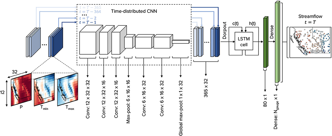
Figure 3. Schematic of the CNN-LSTM architecture. Tmax(x, y, t), Tmin(x, y, t), and P(x, y, t) from T−365 ≤ t ≤ T−1 are input frame-wise through a time-distributed CNN, creating a series of 365 feature vectors each with length 32, where t is time (day) and T is the day of streamflow being predicted. The series of feature vectors is input to an LSTM with 80 units. c(t) and h(t) are the cell and hidden states, respectively. The output of the LSTM is h(t = T−1), which is passed through a final dense layer with linear activation to predict streamflow at Ngauge stations at time t = T. Ngauge is the number of stream gauge stations being predicted by the model, and depends on the stream gauge cluster.
The CNN-LSTM model is driven by coarse resolution temperature and precipitation as input data (0.75° × 0.75°, or ~75 km resolution), with no other meteorological (e.g., solar radiation, wind, humidity) or geographic information (e.g., topography, land use, glacier coverage). The model was designed as a relatively simple proof-of-concept model capable of learning from spatially discretized information to predict streamflow across different streamflow regimes. The model's simulations, i.e., the ensemble mean for each subregional cluster, achieves good performance over the testing dataset, with a median NSE of 0.68 across all stations in the study region, and 35% of stations with NSE>0.8 indicating very good performance. As shown in Anderson and Radić (2022), the model learns that (i) above-freezing temperatures are linked to the onset of the freshet, (ii) the model is often sensitive to input data perturbations in the areas near the basins where streamflow is being predicted, and (iii) summer streamflow in glaciated basins is linked to summer temperature over monthly timescales. Furthermore, there are no explicit climate downscaling steps, and instead the model learns to directly map the coarse-resolution temperature and precipitation data to streamflow. It is suggested that an effective downscaling of climate data may have been learned by the model, which is a plausible hypothesis considering that CNNs have previously been used for downscaling of precipitation data (Vandal et al., 2017). In this study we do not aim to expand or further develop this model by including additional input variables or by changing the architecture; rather, we will investigate how well even the relatively simple proof-of-concept model learns human-interpretable and physically-consistent information.
Experiment on Model's Spatial Learning
The goal of this experiment is to investigate if the model has learned to focus on physically relevant areas or locations of the input domain. By “physically relevant” we mean areas that overlap or are in close proximity to the station where streamflow is being modeled. We also assume that these relevant areas may change through the year since the physical drivers of flow change through the year (e.g., melt, rain, and baseflow). For each streamflow regime, we generate sensitivity maps for each individual day in the testing dataset to detect where and when the model is most sensitive to perturbation in the input data. The experiment consists of systematically perturbing the input variables within a small area of the input domain, and calculating the modeled per-station streamflow response to this perturbation. The response is assessed relative to the original (unperturbed) modeled per-station streamflow. The perturbation field is scaled by the per-station streamflow response to create per-station sensitivity maps. In this way, each station will have a sensitivity map for each day of modeled streamflow, revealing the locations in the input fields where the modeled streamflow is sensitive to perturbation, as well as the magnitude of this sensitivity.
Mathematically, we introduce a perturbation by which we then determine the perturbed input, perturbed output, and sensitivity map for a single stream gauge station and single day as:
where p(x, y) is the perturbation over the whole domain, β is a random factor of ±1 (equal chance of either sign), x and y are longitude and latitude, respectively, xp and yp are the longitude and latitude of the perturbation mid-point, σx and σy are the standard deviations of the Gaussian curve in the x- and y- directions, Tmax, p(x, y, t), Tmin, p(x, y, t), and Pp(x, y, t) are the perturbed input variables, is the predicted model streamflow of the perturbed input, and yflow is the predicted model streamflow of the non-perturbed input, f(·) represents the CNN-LSTM mapping from a weather video to streamflow, and si(x, y) is the sensitivity map for a single perturbation, stream gauge station, and day. p(x, y) has a maximum amplitude of 1, and because each input variable is by scaled by its standard deviation over the training period, the maximum perturbation corresponds to a single standard deviation of each input variable. σx = σy = 1.5 grid cells, limiting the spatial extent of the perturbation to a relatively small area of the input domain.
Next, we generate a mean sensitivity map, S(x, y), for each individual day in the testing dataset, by iterating through equations (1)–(6) for multiple different spatial perturbations p(x, y) with different values of xp and yp. In this way we generate a set of s(x, y) from which we then calculate S(x, y) as:
where Niter is the number of iterations. We iterate until S(x, y) no longer substantially changes through additional perturbation, i.e., when the mean relative error between sensitivity maps from subsequent perturbations is <0.5%. Overall, we calculate Ntest different sensitivity maps S(x, y) for each stream gauge station, where Ntest is the number of days in the testing dataset, i.e., 2011–2015. For each subregional cluster of stream gauge stations, we apply temporal clustering to the Ntest sensitivity maps using agglomerative hierarchical clustering with Ward's method (Hastie et al., 2009). This temporal clustering of sensitivity maps helps us identify the characteristic spatial patterns of sensitivity for each streamflow regime and reveal their evolution through time.
Experiment on the Importance of Input Variables
Our goal here is to determine how strongly the model output is linked to temperature and precipitation separately, and to reveal how the strength of those links change over a year. These links are different across streamflow regimes and change through the year since the physical drivers of flow change through the year (Figure 2). In this experiment we perturb the input temperature and precipitation channels independently to determine if, when, and where the model is sensitive to perturbations of the input weather channels. The steps of the experiment are the same as in section Experiment on Model's Spatial Learning, but here we perturb the temperature and precipitation fields separately. In this way, each station will have its daily sensitivity map to temperature and its daily sensitivity map to precipitation, revealing the relative importance of the two variables and how this importance evolves in time. For the final display of sensitivity maps we will use the six subregional clusters and perform the temporal clustering as described for the previous experiment.
We perturb one of [Tmax, Tmin] or P while keeping the other variable(s) unchanged (e.g., we add a spatial perturbation p(x, y) to Tmax(x, y, t) and Tmin(x, y, t) but not P(x, y, t), and vice versa). We perturb Tmax and Tmin together to ensure physical consistency (e.g., Tmax>Tmin).
Mathematically, the two perturbation scenarios can be described as:
where is modeled streamflow when the temperature channels are perturbed and the precipitation channel is not, and is modeled streamflow when the precipitation channel is perturbed while the temperature channels are not. Then, we calculate sensitivity maps for a single perturbation of each perturbation scenario:
where is a sensitivity map of iteration i when temperature channels are perturbed, and is a sensitivity map of iteration i when the precipitation channel is perturbed. We generate a mean sensitivity map for each of [Tmax, Tmin] and P by iterating through equations (8)–(11) for multiple different spatial perturbations. In both cases, we iterate through until the sensitivity maps converge as defined in section Experiment on Model's Spatial Learning:
where NT and NP are the number of iterations under the perturbed temperature and precipitation scenarios, respectively. ST(x, y) and SP(x, y) are sensitivity maps for a single day, and we calculate sensitivity maps for each of the Ntest days in the testing dataset. We calculate the maximum daily sensitivity, ST, max(t) and SP, max(t), respectively, from the series of sensitivity maps. ST, max(t) and SP, max(t) are measures of the sensitivity through time of the model's predictions to perturbations in temperature and precipitation, respectively, and they indicate the relative importance of temperature and precipitation for predicting streamflow for each day. For each stream gauge cluster, we normalize the maximum sensitivity time series ST, max(t) and SP, max(t) to have maximum values of 1. In this way, the relative importance through the year of temperature and precipitation can be compared, i.e., ST, max(t) = 1 and SP, max(t) = 1 occur on the days when the models are most sensitive to temperature and precipitation perturbations, respectively. Finally, we evaluate how the sensitivity to temperature and precipitation vary throughout a year for each streamflow regime in order to characterize how the learned runoff generation mechanisms compare to the observed streamflow (Figure 2).
Identification of Streamflow-Activating Daily Weather Anomalies
Here we explore how well the model has learned that the streamflow sensitivity to anomalous weather conditions, which drive substantial day-to-day increases in runoff, vary by streamflow regime and season (Figure 2). We start by identifying the temperature and precipitation anomalies that the model associates with day-to-day modeled daily streamflow increases. To do so, we identify the input weather fields that are associated with the maximum single-day increase in output neuron values. For each stream gauge station, we calculate the daily change in modeled streamflow. Consider an example where modeled streamflow at station j increases between days t−1 and t (Supplementary Figure 2). Temperature and precipitation from days t−366 through t−2 are used to model streamflow at day t−1, while temperature and precipitation from days t−365 through t−1 are used to model streamflow at day t. This means that temperature and precipitation at day t−1 is new information to the model for predicting flow at day t. If yflow(t)>yflow(t−1), then Tmax(x, y, t−1), Tmin(x, y, t−1), and P(x, y, t−1) are important for the model's decision that streamflow should increase. While the order of the input sequence has also changed (e.g., input variables are 1 day earlier in the sequence for predicting streamflow at time t as compared to at time t−1), here we focus on the values of temperature and precipitation at time t−1.
We identify the days with the 10% largest single day increases of modeled streamflow for each station and each season [December-January-February (DJF), March-April-May (MAM), June-July-August (JJA), September-October-November (SON)]. Then, we calculate the basin-averaged temperature and precipitation anomalies for the day that precedes each of the top 10% of flow increase days, identifying the per-basin antecedent weather anomalies that cause the model to predict that streamflow should increase. Temperature and precipitation anomalies are calculated by first removing the seasonal cycle of each variable. Then, the residual timeseries of each variable is divided by its standard deviation (Supplementary Figure 4). In this way the anomalies indicate by how much temperature and precipitation have deviated from the average value of that day at each grid cell, relative to the normal variability of that day and grid cell. Finally, we evaluate how the flow-driving antecedent temperature and precipitation vary by season for each streamflow regime to characterize the learned runoff-generation mechanisms, and we compare with a conceptual understanding of the key drivers of flow (Figure 2).
Discovery and Interpretation of Glacier-Runoff Cell States
It is challenging to visually find and interpret LSTM cell states (e.g., as in Karpathy et al., 2015) when there are many states within a single model and many models within an ensemble, as the representation of a hydrological state of interest may be distributed across multiple cell states of which none individually may be similar to the hydrological state of interest. In our case, there are 80 cell states per model and 10 fine-tuned models for each of the six subregions, so we ask: how can we discover physically-interpretable cell states? We assume that some cell states in LSTM models represent water storage or flux terms (e.g., as shown in Kratzert et al., 2018). Furthermore, since glacier melt is an important contributor to streamflow in glaciated rivers, we expect to find a representation of glacier melt within a set of cell states in our model. We design an approach to identify and interpret the LSTM cell states that indirectly represent glacier runoff, without any estimates of actual glacier runoff.
In the CNN-LSTM model, streamflow is predicted simultaneously at multiple different stream gauge stations. This means that a common set of 80 cell states within the LSTM component of the model undergo different linear combinations in the final dense layer to model streamflow at different stations. Glacierized basins are unique in that glacier melt contributes to streamflow even after the seasonal snowpack has melted; in other words, melt drives streamflow through summer in glacierized basins while it does not in non-glacierized basins. Additionally, glacier melt is a more important constituent of streamflow for basins with greater glacier coverage (e.g., Fountain and Tangborn, 1985). Since the importance of glacier melt increases with increasing glaciation, the cell states that are linked to glacier runoff should be more strongly linked to basins with larger fractions of glacier cover.
To identify the cell states linked to glacier runoff we consider the parameters in the final dense layer that relate the LSTM cell states to the neurons in the output layer of the CNN-LSTM model. The cell states that are linked to glacier runoff should be more strongly connected to output neurons (modeled streamflow) of more highly glaciated basins than to those of lightly or non-glaciated basins. The weights in the final dense layer connect all cell states to all output neurons and the weight wij indicates the strength of the connection between cell state i and output neuron j. If |wij| is large (small), then cell state i is more (less) important for determining streamflow at stream gauge j. For each cell state i, we calculate the magnitude of Pearson correlation between the weights wij and the glacier coverage Gj at all output neurons (1 ≤ j ≤ N, where N is the number of output neurons), as well as the statistical significance of the correlation as indicated by the p-value. When the correlation between wij and Gj is significant (p < 0.05), then increasing glacier coverage is associated with stronger connections to the cell state i. The cell states that more likely represent glacier runoff are those for which this correlation is significant, as these states matter more for glaciated basins and less for non-glaciated basins.
For this analysis, we consider only the CNN-LSTM models that are fine-tuned for the central region, because this region has the most glaciated basins in the study domain (Figure 1 and Supplementary Table A1). The fine-tuned ensemble of models for the central region uses a common set of cell states to predict streamflow at multiple glaciated stream gauge stations. From each of the 10 models in the ensemble, we take the cell states connected to weights that are most significantly correlated with glacier coverage (p < 0.05). We further analyze these cell states by clustering them into characteristic temporal patterns to detect a pattern that is visually similar to a conceptual seasonal pattern of glacier contributions to streamflow, i.e., smallest cell state values in winter, positive trend over spring and early summer, largest values in late summer, and negative trend in autumn. The pattern of these cell states is also expected to be linked to the seasonal pattern of positive daily temperatures as these are recognized as an indicator of glacier melt (Hock, 2003).
Results
Temporal Patterns of Spatial Sensitivity
The temporal evolution of sensitivity maps, as derived for each cluster, reveals two distinct patterns of spatial sensitivity of streamflow to perturbations in temperature and precipitation (Figure 4 and Supplementary Figure 3). One pattern of this sensitivity occurs during high flow periods, while the other occurs during low flow periods (Figure 4). The most sensitive areas of the “high-flow” pattern overlaps the basins where streamflow is being predicted (Figure 4, right column). This indicates that when streamflow is most substantial and most dynamic, the model is most sensitive to perturbations in the input data within the basin areas. In contrast, the most sensitive areas of the “low flow” sensitivity maps do not necessarily overlap the basins. In fact, all “low-flow” sensitivity maps are sensitive to perturbations in the input data offshore of the west coast. Furthermore, the evolution of the sensitivity maps reveals that the model is sensitive in a given region for several months at a time, and the sensitivity does not frequently alternate throughout the year between the high-flow and low-flow patterns. This overall behavior is found for all clusters except for the eastern cluster, where the model does not transition from the low-flow pattern to the high-flow pattern until after the spring freshet has already occurred. Thus, for the eastern region, the model is most sensitive to perturbations in the input fields offshore the west coast when it is trying to predict spring flow.
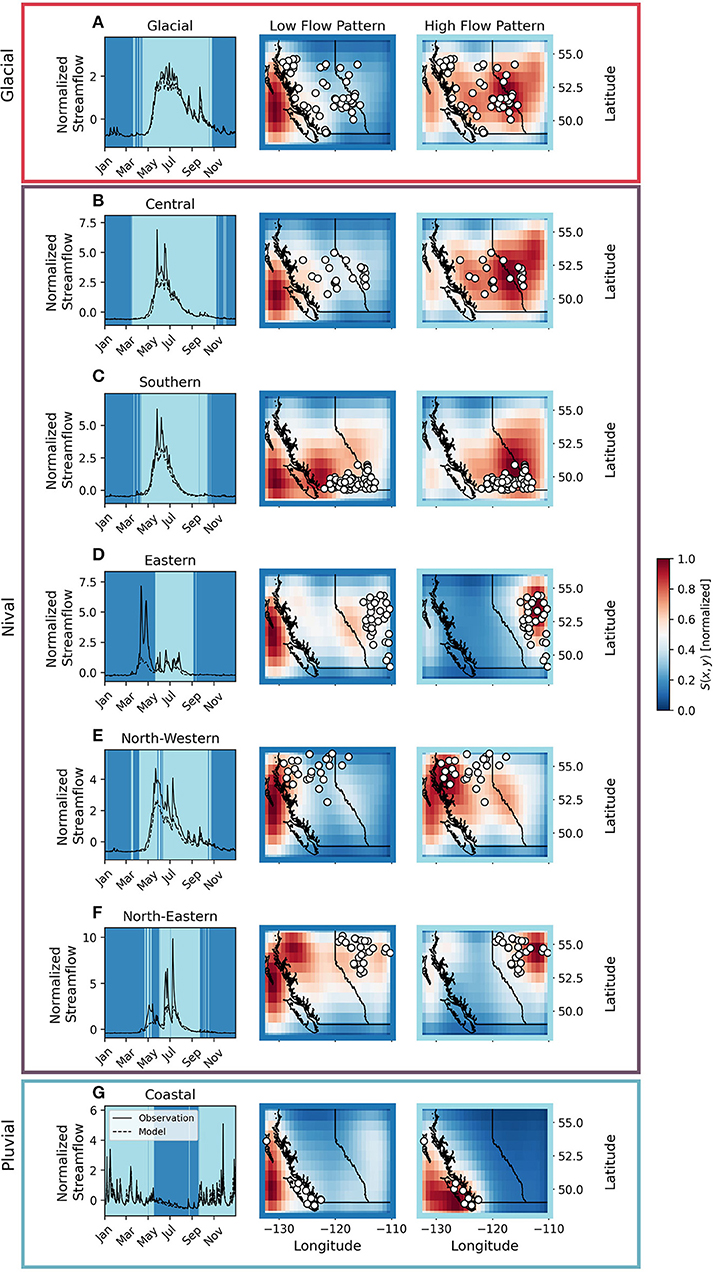
Figure 4. The two characteristic patterns of spatial sensitivity and their occurrence through time for each of the six streamflow clusters. Rows (A–G) display results for nival, glacial, and pluvial sets of stream gauges. Left column: modeled and observed mean streamflow as spatially averaged across stations belonging to the cluster (white circles). Middle column: the “low-flow” sensitivity pattern S(x,y); red indicates areas with high sensitivity to perturbations in input fields. The occurrence of this “low-flow” pattern in time is shown by a dark blue shaded area in the left panel. Right column: the “high-flow” sensitivity pattern S(x,y). The occurrence of this “high-flow” pattern in time is shown by a light blue shaded areas in the left panel. Each sensitivity map S(x,y) is normalized to have a minimum value of 0 and a maximum value of 1.
Importance of Input Variables Through Time
For glacial and nival regimes, ST, max(t) and SP, max(t) are similar during the beginning of the freshet, indicating that the model has learned that the relative importance of temperature is similar to the relative importance of precipitation when predicting the large melt-driven freshet flows (Figure 5). For these two regimes, SP, max(t) and ST, max(t) are smallest during winter, indicating that the model has learned that streamflow is relatively insensitive to temperature and precipitation perturbations, as the subfreezing temperatures suppress streamflow during winter (Figures 2f,k). SP, max(t)>ST, max(t) after the freshet in the eastern, north-eastern, and north-western regions and during fall in the coastal region, consistent with the understanding that rain is driving streamflow and precipitation is not stored as snow (Figures 2e,i,j). In the pluvial regime, the relative importance of precipitation dominates over temperature for the bulk of the year.
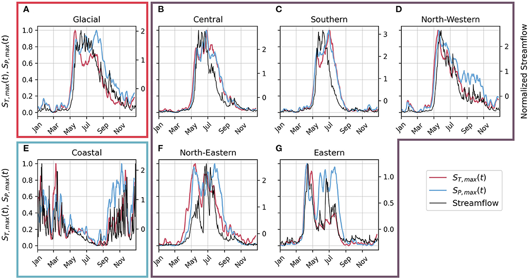
Figure 5. The daily maximum sensitivity to temperature and precipitation perturbations (ST, max(t) and SP, max(t)) alongside observed streamflow for each of the stream gauge clusters. A single year in the testing dataset (2011) is shown as an example. The clusters belonging to the glacial (A), nival (B,C,D,F,G), and pluvial (E) regimes are indicated by the bounding boxes.
Streamflow-Activating Daily Weather Anomalies
For each streamflow regime we calculate seasonal distributions of daily temperature and precipitation anomalies that precede the largest modeled flow increases (Figure 6). During winter and spring in melt-driven nival and glacial regimes, modeled streamflow increases following warm but not necessarily wet anomalies (Figures 6A,B), consistent with snowmelt-driven flows (Figures 2h,m). In contrast, modeled streamflow increases follow wet but not necessarily warm anomalies in the pluvial regime, consistent with rainfall-driven flows (Figure 2b). During summer in nival and pluvial basins, modeled streamflow increases following cool and wet anomalies (Figure 6C), consistent with the knowledge that rainy summer days are cooler and wetter than average summer days. In glacial basins, warmer than average temperatures precede modeled streamflow, but both wet and dry anomalies can precede streamflow increases in glacial basins. This learned behavior is consistent with the understanding that both rainfall and glacier melt can drive streamflow during summer in glacial basins (Figures 2o,p). During fall, modeled streamflow increases following wet and warm anomalies in all regimes (Figure 6D), consistent with rainfall- (pluvial, nival, or glacial regimes; Figures 2e,j,o) or melt-driven flows (glacial regime; Figure 2p). The coastal basins are the only set of stations that the model has learned that wet precipitation anomalies precede an increase in flow in all seasons (Figure 6), consistent with the known rainfall-driven regime.
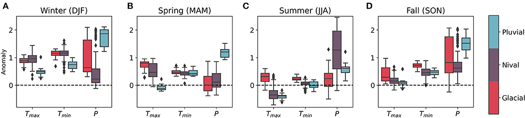
Figure 6. Daily anomalies of maximum temperature, minimum temperature, and precipitation, preceding the largest day-to-day modeled flow increases in (A) winter, (B) spring, (C) summer, and (D) fall. Results are presented by streamflow regime (pluvial, nival and glacial). The dashed black line indicates zero (or average) values. Positive values indicate warmer or wetter than average, while negative values indicated colder or drier than average.
The same experiment is used to determine if the model has learned that daily-scale streamflow is more driven by warm anomalies in more highly glaciated basins indicative of melt-driven streamflow, rather than by wet anomalies indicative of rainfall-driven streamflow. We consider only the summer months (JJA) when glacier runoff is greatest. We find that warmer and drier anomalies precede a rise in modeled flow in more highly glaciated basins, while colder and wetter anomalies precede a rise in modeled flow in less glaciated basins in summer (Figure 7). These findings indicate that the model has learned that large streamflow events are driven by different processes in glaciated basins as compared to non-glaciated basins, consistent with the understanding that glacier melt is an important constituent of streamflow in glaciated basins.
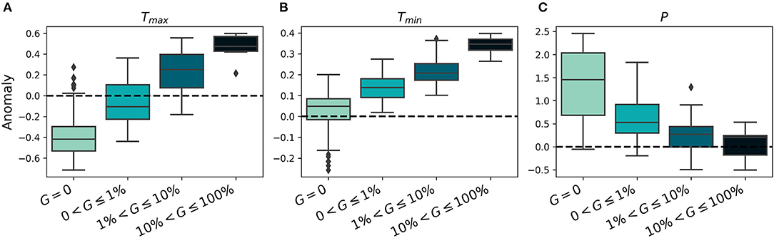
Figure 7. Box plots of daily anomalies of (A) maximum temperature, (B) minimum temperature, and (C) precipitation that precede modeled flow increases in summer, for a given fraction of per-basin glacier cover (G). The dashed black line indicates zero (or average) values. Positive values indicate warmer or wetter than average, while negative values indicate cooler or drier than average. We divide basins into four bins of glacier coverage (no glacier coverage: G = 0; light glacier coverage: 0 < G ≤ 1%; moderate glacier coverage: 1% < G ≤ 10%; and high glacier coverage: 10% < G ≤ 100%).
Cell States Linked to Glacier Runoff
For the ensemble of 10 models fine-tuned for the central region, we identified 106 (out of the 800) cell states whose weights are significantly correlated with basin glacier coverage (p < 0.05). The mean correlation coefficient between the weights in the final dense layer in the CNN-LSTM model and the basin glacier coverage for these 106 “glacially-relevant” cell states is 0.35 (minimum correlation of 0.27, maximum correlation of 0.51). Out of these 106 cell states we investigate one set of 56 states whose seasonal pattern resembles the idealized seasonal pattern of glacier runoff (Supplementary Figures 5, 6). The mean pattern, averaged across those cell states, is then compared with positive daily mean temperatures, derived from ERA5 data as a spatial mean over the central region (Figure 8A). The seasonal pattern of daily temperatures shows minimum values in the winter months, then an increase from late April through early August, and then a decrease until November. The cell state pattern, however, increases from early June through August, and then decreases until November (Figure 8A). We remove the 30-day running mean from both time series to investigate the cross-correlation between the daily-scale fluctuations of positive temperatures and the cell state cluster pattern. We find that correlation between the two residuals is maximized when the positive temperature residuals lead the cell state residuals by 2 days (Figure 8B). The correlation between the residuals with the 2-day lag is 0.55 over the year; for comparison, the correlation is 0.47 for a 3-day lag, 0.46 for a 1-day lag, and 0.11 for no lag.
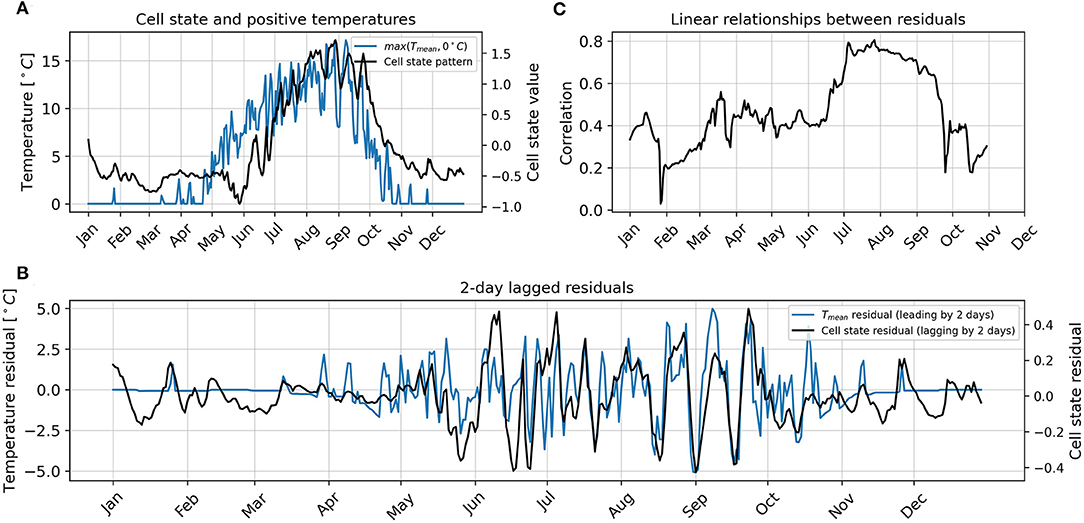
Figure 8. The representation of glacier runoff in LSTM cell states. (A) Positive mean daily temperatures, calculated as an average over the central region, and the mean cell state pattern of the glacier-runoff-like set of cell states. (B) The lagged residuals of mean temperature and the cell state pattern, as calculated by removing the 30-day running mean of each time series in (A). (C) The correlation between temperature residuals and 2-day-lagged cell state residuals for each 60-day running window through the year.
In addition to the cross-correlation analysis over the whole year, we investigate shorter time windows throughout the year. For this analysis, we use a running 60-day window, and calculate the correlation coefficient between the 2-day lagged residuals over each window (Figure 8C). We find that the correlation, with a 2-day lag, is greatest between approximately mid-June through mid-September. During this period, the average Pearson correlation coefficient is approximately 0.70, as compared to 0.37 throughout the rest of the year.
Discussion
The CNN-LSTM model is not given any information other than gridded temperature and precipitation for predicting streamflow at multiple stations across the region (e.g., climatic, geographic, or topographic variables). Yet we demonstrate that the model, in this process of learning to simultaneously model streamflow at different stations, has learned human-interpretable links between the input and output variables. In particular, the sensitivity experiments reveal three characteristics of the model's learning that resemble those expected from a conceptual understanding of the hydrological processes (Figure 2). Here we highlight three characteristics of the model's learning that demonstrate that the learned temporal variation of streamflow sensitivity to perturbations in temperature and precipitation, as well as the learned temporal variation of daily weather anomalies that drive runoff generation, are both streamflow regime specific. Firstly, the model learns that the mechanism that generates runoff can vary through time for a particular streamflow regime. The nival eastern, north-eastern, and north-western basins have a snowmelt-driven freshet in spring and rainfall-driven flows in late spring, summer, or fall (Figures 1B,C,E). For these basins, both temperature and precipitation are highly important for predicting flow during the spring freshet (Figures 5C,E,F) and warm temperature anomalies precede modeled flow increases (Figure 6B), all of which is consistent with the understanding that the timing and magnitude of flow is governed primarily by snowmelt (Figures 2g,h). Then, as the basins transition to being driven by rainfall, precipitation becomes a more important predictor (Figures 5C,E,F) and wet anomalies precede modeled flow increases (Figure 6C), indicating that the model has learned that the runoff generating mechanism has changed and is now more strongly linked to precipitation rather than temperature (Figures 2i,j). Secondly, the model learns that the runoff generating mechanism can vary through space across different streamflow regimes. Nival and glacial basins are predominantly driven by melt (Figures 2g,l), while pluvial basins are predominantly driven by rain (Figures 2a,e). That the learned runoff generating mechanisms are different between the nival and glacial regimes as compared to the pluvial regime is revealed by the different antecedent weather conditions that drive flow during the spring freshet (Figure 6B). The model has learned to link warm and dry anomalies with streamflow increases in glacial and nival rivers, indicative of melt, while at the same time linking cold and wet anomalies with streamflow increases in pluvial rivers, indicative of rainfall-driven flows. Thirdly, we find that the model learns that the runoff generating mechanism can vary across a latent variable unknown to the model during training; in our case, basin glacier coverage. The model has automatically learned that the runoff generating mechanisms in summer vary across a range of glacier coverage (Figure 7), consistent with glacier melt generating the most substantial modeled streamflow events in more highly glaciated basins (Figure 2n).
Our findings that the model learns regime-specific sensitivity to perturbations in the input fields corroborate previous findings by Wunsch et al. (2022) who used a CNN-LSTM model for streamflow prediction in three karst catchments. Their model is shown to be more sensitive to perturbations in precipitation as compared to temperature and radiation for a basin that is predominantly driven by rainfall, while the model is more sensitive to perturbations in snowmelt as compared to precipitation for a basin that has important snowmelt contributions (Wunsch et al., 2022). In our study, we go a step further by demonstrating that the model's sensitivity to perturbations in the input variables not only varies across different streamflow regimes, as in Wunsch et al. (2022), but that it can also vary both through time and across a latent variable unknown to the model during training. Furthermore, we also show that the model has learned to differentiate between different melt sources (e.g., between the runoff-generating mechanisms of glacier-melt and snow-melt driven flows), despite not giving any information on the source of melt (seasonal snow or glacier) to the model. In fact, without giving any information on glacier cover per basin, the model learned that the streamflow sensitivity to warm daily anomalies in late summer will increase with the increase in fraction of glacier cover per basin (Figure 7).
We explain how the model's decision making varies across differently glaciated basins by identifying a set of internal cells in the LSTM model that can be interpreted as a proxy for glacier runoff. These internal cell states have the highest correlation between their daily fluctuations and the 2-day lagged fluctuations of daily temperature (Figure 8). Physically, the 2-day lag could represent the travel time that it takes for surface glacier melt to travel first through the glacier system, with an hourly (sub-daily) response time (e.g., Burkimsher, 1983; Jansson et al., 2003), and then through the basin's stream network, with a daily response time (e.g., McGuire and McDonnell, 2006; Attard et al., 2014). Importantly, this relationship between daily positive temperature and streamflow is strongest in late summer (Figure 8C) when glacier melt is maximized (e.g., Hock, 2005; Figure 2n), and for basins with greater glacier coverage (Figure 7). This identified cell state pattern can be interpreted as a temperature-dependent streamflow source that is activated for glacial basins, and that is most strongly linked to positive temperature during the glacier melt season. We note that our method to identify and interpret these LSTM cell states is different than prior examples in hydrology. While Kratzert et al. (2019a) correlate cell states directly with hydrological states of interest (soil moisture and snow water equivalent), we identify and interpret the cell states through their links with an indicator (basin glacier coverage) of the hydrological state of interest (glacier runoff), and then through their similarity with an idealized pattern of glacier runoff. By identifying and interpreting the cell states in this way, we circumvent the need to know the observed glacier runoff for each basin, data that is not available for this region and is generally hard to obtain through observations or modeling on a regional scale (e.g., Radić and Hock, 2014). Here we leverage glacier coverage and runoff to interpret the LSTM cell states, while previously LSTMs have primarily been applied for regional streamflow prediction in regions where relatively few basins are glaciated (e.g., Kratzert et al., 2019c; Feng et al., 2020; Xiang et al., 2020; Gauch et al., 2021). As such there has been limited consideration of how glaciers modulate the learned streamflow response and internal model parameters, i.e., the same meteorological forcing (input to the LSTM) produces a different streamflow response (output of the LSTM) in a glaciated basin as compared to a non-glaciated basin, necessitating different internal model decision making between the two cases.
Glacier runoff has not been explicitly considered by deep learning models developed for either regional streamflow prediction, or for glaciological applications. To our knowledge, our study is the first application of deep learning in hydrology with specific considerations of glacier runoff (Shen et al., 2021), despite wider use of deep learning in hydrology and a growing number of applications in glaciology (Liu, 2021). Deep learning in glaciology has been primarily developed for classification tasks using remote sensing data due to the large volumes of data available (e.g., Xie et al. Nijhawan et al., 2018; Baumhoer et al., 2019; Robson et al., 2020; Taylor et al., 2021). Applications of deep learning for regression tasks, rather than classification, are scarcer, and have so far been restricted to the most data-rich regions such as the French Alps (e.g., Bolibar et al., 2020a,b, 2022). One reason for this restriction is the limited availability of long-term observations in many glacierized regions for training deep learning models. There is opportunity for the further development and investigation of deep learning models in glacier hydrology because of the wider availability of streamflow data and globally available glacier inventories (RGI Consortium, 2017), as we demonstrate that these data sets together can be leveraged to gain insights from deep learning hydrological models.
In this study we investigate glacier runoff in particular because of its importance as a contributor to streamflow in the study region. More generally, deep learning models should be interpreted under the conditions and context for which they will be applied. For example, future work could investigate how and if other important processes are represented (e.g., evapotranspiration, groundwater flow), and how these representations are influenced by training models in regions with different geographic and climatic characteristics or by training models over different spatial and temporal scales.
The sensitivity maps used for investigating the model's spatial learning expand upon the earlier findings in Anderson and Radić (2022) that used the same CNN-LSTM model over the same study region as here. As reported in their study, the model was not always sensitive to the perturbation in the input variables within or nearby the basins whose streamflow is being modeled. In fact, for some stations in the region (e.g., in the eastern cluster) the model was more sensitive to the perturbations far away (off-shore the west coast of BC) than within/nearby the basins. Here we demonstrate that this sensitivity to “distant” perturbations in input fields occurs mainly during low-flow periods of the year (Figure 4), when the streamflow sensitivity to temperature and precipitation is low or negligible (Figure 5). As soon as streamflow becomes more dynamic (e.g., during the freshet), the model re-focuses on the climatic drivers within/nearby the modeled streamflow and maintains this focus until the streamflow becomes more dormant again in the late fall and winter. The only exception to this finding is the eastern cluster where the model continues to focus on the “distant” climate forcing (west coast of BC) through the freshet period. The eastern cluster is situated in the Prairie Pothole Region which is characterized by small surface depressions that allow for dynamical water storage and intermittent connectivity which can vary on both seasonal and decadal timescales (Shook and Pomeroy, 2011; Shaw et al., 2012; Hayashi et al., 2016). This level of complexity in runoff generation, characteristic of the eastern region, may “mask” the links between the local weather variables and streamflow, justifying the model's “poor learning” in this sub-region. Data integration that incorporates previous streamflow into the input data has been found to improve LSTM model performance in the Prairie Pothole Region of the United States (Feng et al., 2020). Future work can investigate if improvements to model performance, such as through incorporation of additional information (e.g. topography, radiative forcing, surface water storage, previous streamflow), also alters the spatiotemporal patterns of model sensitivity.
Summary and Conclusion
We investigated the interpretability of the previously trained CNN-LSTM model from Anderson and Radić (2022) used for streamflow simulations at 226 stream gauge stations across southwestern Canada. Forced only by the gridded daily temperature and precipitation fields from ERA5 reanalysis, the model was shown to successfully simulate observed daily streamflow between 1980 and 2015 (Anderson and Radić, 2022). Here we designed a set of experiments to assess the model's sensitivity to spatiotemporal perturbations in temperature and precipitation fields. With these sensitivity tests, we probed the model's ability to learn runoff-generating mechanisms across three main streamflow regimes in the region: glacial, nival, and pluvial. Our results reveal that the model has learned the basic principles behind the runoff generation for each streamflow regime, without being given any information other than temperature, precipitation, and streamflow data. We show that:
1. The model is more sensitive to the perturbations while the streamflow is dynamic, i.e., from the onset of freshets in spring until the start of subfreezing temperatures in late fall or early winter. During this period of “dynamic flow,” the model is more sensitive to the perturbations within/nearby the basins, whose streamflow is being modeled, than to the perturbations far away from the basins. The only exception to this sensitivity pattern is found for the eastern subregion (Prairies in Alberta), where the model's counter-intuitive sensitivity to distant perturbations (off-shore the west coast of British Columbia) during freshets is likely attributed to the presence of more complex water-storage systems in the subregion relative to the rest of the study region.
2. The model learned that each streamflow regime displays characteristic temporal pattern of sensitivity to the perturbations in temperature and precipitation. During freshets in the nival and glacial regimes, the model is more or equally sensitive to temperature as to precipitation, while sensitivity to precipitation generally dominates over temperature for the rest of the year. In the pluvial regime, the model is more sensitive to precipitation than to temperature throughout the year.
3. The model learned that substantial day-to-day increases in streamflow are triggered by daily anomalies in temperature and precipitation, and the seasonal pattern of this sensitivity to weather anomalies is characteristic for each streamflow regime. For the nival regime, the streamflow increases are driven by warm daily anomalies in spring, and wet daily anomalies in summer. For the glacial regime, warm daily anomalies drive the flow increases in the spring and summer, corresponding to the temperature-driven snow- and glacier-melt contribution to the streamflow.
4. The model learned that daily-scale flow events are increasingly preceded by warm anomalies under increasing fraction of glacier cover per basin. We interpreted this finding by identifying a set of cell states in the LSTM model that act as temperature-controlled streamflow sources in summer, i.e., glacier runoff. These cell states most strongly mapped temperature to streamflow in glacierized basins during the summer months, while at the same time were inactive for the non-glacierized basins.
In conclusion, our results reveal that the decision-making process of the deep-learning model is interpretable and consistent with the known drivers of streamflow. These findings agree with the currently small, but growing number of studies that have explored the interpretability of deep learning models for streamflow prediction (e.g., Kratzert et al., 2019a; Anderson and Radić, 2022; Wunsch et al., 2022). The growing body of evidence that deep learning resembles a physics-based understanding of the hydrological processes can help build confidence in these models beyond their use as “black box” models. Gaining trust in the deep learning models is an important step forward for the hydrological modeling community facing the challenges and opportunities associated with the growing availability of big data at a time of unprecedented risks of water scarcity under climate change.
Data Availability Statement
All data used are publicly available. ERA reanalysis data are from the European Centre for Medium-Range Weather Forecasts (ECMWF) (Hersbach et al., 2020). Streamflow data are from the Environment Canada HYDAT database (Environment Climate Change Canada, 2018). Basin outlines are from the Water Survey of Canada (Environment Climate Change Canada, 2016). Provincial borders are from Statistics Canada (Statistics Canada, 2016). Code to reproduce all figures and results from this study is available on Github (Anderson, 2022).
Author Contributions
SA designed and conducted the study. SA and VR analyzed the results and wrote the paper. Both authors contributed to the article and approved the submitted version.
Funding
This study has been supported through the Natural Sciences and Engineering Research Council (NSERC) of Canada by a Discovery Grant to VR and a Doctoral Scholarship to SA.
Conflict of Interest
The authors declare that the research was conducted in the absence of any commercial or financial relationships that could be construed as a potential conflict of interest.
Publisher's Note
All claims expressed in this article are solely those of the authors and do not necessarily represent those of their affiliated organizations, or those of the publisher, the editors and the reviewers. Any product that may be evaluated in this article, or claim that may be made by its manufacturer, is not guaranteed or endorsed by the publisher.
Supplementary Material
The Supplementary Material for this article can be found online at: https://www.frontiersin.org/articles/10.3389/frwa.2022.934709/full#supplementary-material
References
Abadi, M., Agarwal, A., Barham, P., Brevdo, E., Chen, Z., Citro, C., et al. (2016). TensorFlow: large-scale machine learning on heterogeneous distributed systems. arXiv. doi: 10.48550/arXiv.1603.04467
Abramowitz, G (2005). Towards a benchmark for land surface models. Geophys. Res. Lett. 32, L22702. doi: 10.1029/2005GL024419
Anderson, S (2022). andersonsam/cnn_lstm_interpret: First release (v1.0.0). Zenodo. doi: 10.5281/zenodo.6587601
Anderson, S., and Radić, V. (2020). Identification of local water resource vulnerability to rapid deglaciation in Alberta. Nat. Clim. Chang. 10, 933–938. doi: 10.1038/s41558-020-0863-4
Anderson, S., and Radić, V. (2022). Evaluation and interpretation of convolutional long short-term memory networks for regional hydrological modelling. Hydrol. Earth Syst. Sci. 26, 795–825. doi: 10.5194/hess-26-795-2022
Attard, M. E., Venditti, J. G., and Church, M. (2014). Suspended sediment transport in Fraser River at Mission, British Columbia: new observations and comparison to historical records. Can. Water Res. J. 39, 356–371. doi: 10.1080/07011784.2014.942105
Bach, S., Binder, A., Montavon, G., Klauschen, F., Müller, K.-R., and Samek, W. (2015). On pixel-wise explanations for non-linear classifier decisions by layer-wise relevance propagation. PLoS ONE 10, e0130140. doi: 10.1371/journal.pone.0130140
Baumhoer, C. A., Dietz, A. J., Kneisel, C., and Kuenzer, C. (2019). Automated extraction of antarctic glacier and ice shelf fronts from sentinel-1 imagery using deep learning. Remote Sens. 11, 2529. doi: 10.3390/rs11212529
Best, M. J., Abramowitz, G., Johnson, H. R., Pitman, A. J., Balsamo, G., Boone, A., et al. (2015). The plumbing of land surface models: benchmarking model performance. J. Hydrometeorol. 16, 1425–1442. doi: 10.1175/JHM-D-14-0158.1
Bianchi, F., Rossiello, G., Costabello, L., Palmonari, M., and Minervini, P. (2020). Knowledge graph embeddings and explainable AI. ArXiv abs/2004.14843. doi: 10.48550/arXiv.2004.14843
Bolibar, J., Rabatel, A., Gouttevin, I., and Galiez, C. (2020a). A deep learning reconstruction of mass balance series for all glaciers in the French Alps: 1967–2015. Earth System Sci. Data 12, 1973–1983. doi: 10.5194/essd-12-1973-2020
Bolibar, J., Rabatel, A., Gouttevin, I., Galiez, C., Condom, T., and Sauquet, E. (2020b). Deep learning applied to glacier evolution modelling. Cryosphere 14, 565–584. doi: 10.5194/tc-14-565-2020
Bolibar, J., Rabatel, A., Gouttevin, I., Zekollari, H., and Galiez, C. (2022). Nonlinear sensitivity of glacier mass balance to future climate change unveiled by deep learning. Nat. Commun. 13, 409. doi: 10.1038/s41467-022-28033-0
Bowes, B. D., Sadler, J. M., Morsy, M. M., Behl, M., and Goodall, J. L. (2019). Forecasting groundwater table in a flood prone coastal city with long short-term memory and recurrent neural networks. Water 11, 1098. doi: 10.3390/w11051098
Burkimsher, M (1983). Investigations of glacier hydrological systems using dye tracer techniques: observations at Pasterzengletscher, Austria. J. Glaciol. 29, 403–416. doi: 10.3189/S002214300003032X
Chollet, F (2015). Keras. GitHub Repository. Available online at: https://github.com/fchollet/keras
Daw, A., Thomas, R. Q., Carey, C. C., Read, J. S., Appling, A. P., and Karpatne, A. (2020). “Physics-guided architecture (PGA) of neural networks for quantifying uncertainty in lake temperature modeling,” in Proceedings of the 2020 SIAM International Conference on Data Mining (SDM), 532–540. doi: 10.1137/1.9781611976236.60
Donahue, J., Hendricks, L. A., Rohrbach, M., Venugopalan, S., Guadarrama, S., Saenko, K., et al. (2017). Long-term recurrent convolutional networks for visual recognition and description. IEEE Trans. Pattern Anal. Mach. Intell. 39, 677–691. doi: 10.1109/TPAMI.2016.2599174
Eaton, B., and Moore, R. D. (2010). “Regional Hydrology,” in Compendium of Forest Hydrology and Geomorphology in British Columbia, eds R. G. Pike, T. E. Redding, R. D. Moore, R. D. Winkler, and K. D. Bladon, (Victoria, BC: Ministry of Forests and Range), 85–110. Available online at: https://www.for.gov.bc.ca/hfd/pubs/docs/lmh/Lmh66.htm (accessed February 10, 2022).
Environment Climate Change Canada (2016). National Hydrometric Network Basin Polygons. Available online at: https://open.canada.ca/data/en/dataset/0c121878-ac23-46f5-95df-eb9960753375
Environment Climate Change Canada (2018). Water Survey of Canada HYDAT Data. Available online at: https://wateroffice.ec.gc.ca/mainmenu/historical_data_index_e.html
Fang, K., Shen, C., Kifer, D., and Yang, X. (2017). Prolongation of SMAP to spatiotemporally seamless coverage of continental U.S. using a deep learning neural network. Geophys. Res. Lett. 44, 11–30. doi: 10.1002/2017GL075619
Feng, D., Fang, K., and Shen, C. (2020). Enhancing streamflow forecast and extracting insights using long-short term memory networks with data integration at continental scales. Water Resour. Res. 56, e2019WR026793. doi: 10.1029/2019WR026793
Fleming, S. W., Garen, D. C., Goodbody, A. G., McCarthy, C. S., and Landers, L. C. (2021a). Assessing the new Natural Resources Conservation Service water supply forecast model for the American West: a challenging test of explainable, automated, ensemble artificial intelligence. J. Hydrol. 602, 126782. doi: 10.1016/j.jhydrol.2021.126782
Fleming, S. W., Vesselinov, V. v., and Goodbody, A. G. (2021b). Augmenting geophysical interpretation of data-driven operational water supply forecast modeling for a western US river using a hybrid machine learning approach. J. Hydrol. 597, 126327. doi: 10.1016/j.jhydrol.2021.126327
Fountain, A. G., and Tangborn, W. v. (1985). The effect of glaciers on streamflow variations. Water Resour. Res. 21, 579–586. doi: 10.1029/WR021i004p00579
Frame, J., Kratzert, F., Klotz, D., Gauch, M., Shelev, G., Gilon, O., et al. (2021). Deep learning rainfall-runoff predictions of extreme events. Hydrol. Earth Syst. Sci. Discuss. 2021, 1–20. doi: 10.5194/hess-2021-423
Frans, C., Istanbulluoglu, E., Lettenmaier, D. P., Clarke, G., Bohn, T. J., and Stumbaugh, M. (2016). Implications of decadal to century scale glacio-hydrological change for water resources of the Hood River basin, OR, USA. Hydrol. Process. 30, 4314–4329. doi: 10.1002/hyp.10872
Gagne, D. J. II., Haupt, S. E., Nychka, D. W., and Thompson, G. (2019). Interpretable deep learning for spatial analysis of severe hailstorms. Monthly Weather Rev. 147, 2827–2845. doi: 10.1175/MWR-D-18-0316.1
Gauch, M., Kratzert, F., Klotz, D., Nearing, G., Lin, J., and Hochreiter, S. (2021). Rainfall–runoff prediction at multiple timescales with a single Long Short-Term Memory network. Hydrol. Earth Syst. Sci. 25, 2045–2062. doi: 10.5194/hess-25-2045-2021
Hastie, T., Tibshirani, R., and Friedman, J. H. (2009). The Elements of Statistical Learning: Data Mining, Inference, and Prediction, 2nd Edn. New York, NY: Springer. Available online at: https://adams.marmot.org/Record/.b41452057#:~:text=Hastie%2C T.%2C Tibshirani%2C,New York%3A Springer
Hayashi, M., van der Kamp, G., and Rosenberry, D. O. (2016). Hydrology of prairie wetlands: understanding the integrated surface-water and groundwater processes. Wetlands 36, 237–254. doi: 10.1007/s13157-016-0797-9
Hersbach, H., Bell, B., Berrisford, P., Hirahara, S., Horányi, A., Muñoz-Sabater, J., et al. (2020). The ERA5 global reanalysis. Q. J. R. Meteorol. Soc. 146, 1999–2049. doi: 10.1002/qj.3803
Hochreiter, S., and Schmidhuber, J. (1997). Long short-term memory. Neural Comput. 9, 1735–1780. doi: 10.1162/neco.1997.9.8.1735
Hock, R (2003). Temperature index melt modelling in mountain areas. J. Hydrol. 282, 104–115. doi: 10.1016/S0022-1694(03)00257-9
Hock, R (2005). Glacier melt: a review of processes and their modelling. Progress Phys. Geogr. 29, 362–391. doi: 10.1191/0309133305pp453ra
Hoedt, P.-J., Kratzert, F., Klotz, D., Halmich, C., Holzleitner, M., Nearing, G., et al (2021). MC-LSTM: Mass-Conserving LSTM. Available online at: https://arxiv.org/abs/2101.05186 (accessed August 22, 2021).
Hsu, K., Gupta, H. V., and Sorooshian, S. (1995). Artificial neural network modeling of the rainfall-runoff process. Water Resour. Res. 31, 2517–2530. doi: 10.1029/95WR01955
Hu, C., Wu, Q., Li, H., Jian, S., Li, N., and Lou, Z. (2018). Deep learning with a long short-term memory networks approach for rainfall-runoff simulation. Water 10, 1543. doi: 10.3390/w10111543
Jansson, P., Hock, R., and Schneider, T. (2003). The concept of glacier storage: a review. J. Hydrol. 282, 116–129. doi: 10.1016/S0022-1694(03)00258-0
Jia, X., Willard, J., Karpatne, A., Read, J., Zwart, J., Steinbach, M. S., et al. (2019). “Physics guided RNNs for modeling dynamical systems: A case study in simulating lake temperature profiles,” in SIAM International Conference on Data Mining, SDM 2019 (Society for Industrial and Applied Mathematics Publications), 558–566. doi: 10.1137/1.9781611975673.63
Karpathy, A., Johnson, J., and Li, F.-F. (2015). Visualizing and understanding recurrent networks. arXiv. doi: 10.48550/arXiv.1506.02078
Karpatne, A., Watkins, W., Read, J., and Kumar, V. (2017). Physics-guided Neural Networks (PGNN): an application in lake temperature modeling. ArXiv. doi: 10.48550/arXiv.1710.11431
Kingma, D. P., and Ba, J. (2017). Adam: a method for stochastic optimization. ArXiv. doi: 10.48550/arXiv.1412.6980
Kratzert, F., Herrnegger, M., Klotz, D., Hochreiter, S., and Klambauer, G. (2019a). “NeuralHydrology – Interpreting LSTMs in Hydrology,” in Explainable AI: Interpreting, Explaining and Visualizing Deep Learning. Lecture Notes in Computer Science, vol 11700, eds W. Samek, G. Montavon, A. Vedaldi, L. Hansen, and K. R. Müller (Cham: Springer). doi: 10.1007/978-3-030-28954-6_19
Kratzert, F., Klotz, D., Brenner, C., Schulz, K., and Herrnegger, M. (2018). Rainfall–runoff modelling using Long Short-Term Memory (LSTM) networks. Hydrol. Earth Syst. Sci. 22, 6005–6022. doi: 10.5194/hess-22-6005-2018
Kratzert, F., Klotz, D., Herrnegger, M., Sampson, A. K., Hochreiter, S., and Nearing, G. S. (2019b). Toward improved predictions in ungauged basins: exploiting the power of machine learning. Water Resour. Res. 55, 11344–11354. doi: 10.1029/2019WR026065
Kratzert, F., Klotz, D., Shalev, G., Klambauer, G., Hochreiter, S., and Nearing, G. (2019c). Towards learning universal, regional, and local hydrological behaviors via machine learning applied to large-sample datasets. Hydrol. Earth Syst. Sci. 23, 5089–5110. doi: 10.5194/hess-23-5089-2019
Le, X.-H., Ho, H. V, Lee, G., and Jung, S. (2019). Application of long short-term memory (LSTM) neural network for flood forecasting. Water 11, 1387. doi: 10.3390/w11071387
LeCun, Y., Boser, B., Denker, J. S., Howard, R. E., Habbard, W., Jackel, L. D., et al. (1990). “Handwritten digit recognition with a back-propagation network,” in Advances in Neural Information Processing Systems (San Francisco, CA: Morgan Kaufmann Publishers Inc.), 396–404.
Liu, L (2021). “A review of deep learning for cryospheric studies,” in Deep Learning for the Earth Sciences, eds G. Camps-Valls, D. Tuia, X. X. Zhu and M. Reichstein. doi: 10.1002/9781119646181.ch17
Lundberg, S., and Lee, S.-I. (2017). A unified approach to interpreting model predictions. arXiv. doi: 10.48550/arXiv.1705.07874
Maier, H. R., and Dandy, G. C. (2000). Neural networks for the prediction and forecasting of water resources variables: a review of modelling issues and applications. Environ. Modell. Soft. 15, 101–124. doi: 10.1016/S1364-8152(99)00007-9
Maier, H. R., Jain, A., Dandy, G. C., and Sudheer, K. P. (2010). Methods used for the development of neural networks for the prediction of water resource variables in river systems: current status and future directions. Environ. Modell. Softw. 25, 891–909. doi: 10.1016/j.envsoft.2010.02.003
Mayer, K. J., and Barnes, E. A. (2021). Subseasonal forecasts of opportunity identified by an explainable neural network. Geophys. Res. Lett. 48, e2020GL092092. doi: 10.1029/2020GL092092
McGovern, A., Lagerquist, R., John Gagne, D., Jergensen, G. E., Elmore, K. L., Homeyer, C. R., et al. (2019). Making the black box more transparent: understanding the physical implications of machine learning. Bull. Am. Meteorol. Soc. 100, 2175–2199. doi: 10.1175/BAMS-D-18-0195.1
McGuire, K. J., and McDonnell, J. J. (2006). A review and evaluation of catchment transit time modeling. J. Hydrol. 330, 543–563. doi: 10.1016/J.JHYDROL.2006.04.020
Meier, M. F., and Tangborn, W. v. (1961). Distinctive characteristics of glacier runoff. US Geol. Surv. Prof. Pap. 424, B14–B16.
Moore, R. D., Spittlehouse, D. L., Whitfield, P. H., and Stahl, K. (2010). “Weather and climate,” in Compendium of Forest Hydrology and Geomorphology in British Columbia, eds R. G. Pike, T. E. Redding, R. D. Moore, R. D. Winkler, and K. D. Bladon (Victoria, BC: B.C. Ministry of Forests and Range), 47–84. Available online at: https://www.for.gov.bc.ca/hfd/pubs/Docs/Lmh/Lmh66.htm
Nearing, G. S., Kratzert, F., Sampson, A. K., Pelissier, C. S., Klotz, D., Frame, J. M., et al. (2021). What role does hydrological science play in the age of machine learning? Water Resources Res. 57, e2020WR028091. doi: 10.1029/2020WR028091
Nearing, G. S., Mocko, D. M., Peters-Lidard, C. D., Kumar, S.V, and Xia, Y. (2016). Benchmarking NLDAS-2 Soil Moisture and Evapotranspiration to Separate Uncertainty Contributions. Journal of Hydrometeorology 17, 745–759. doi: 10.1175/JHM-D-15-0063.1
Nijhawan, R., Das, J., and Balasubramanian, R. (2018). A Hybrid CNN + random forest approach to delineate debris covered glaciers using deep features. J. Indian Soc. Remote Sens. 46, 981–989. doi: 10.1007/s12524-018-0750-x
Odon, P., West, G., and Stull, R. (2018). Evaluation of reanalyses over British Columbia. Part I: daily and extreme 2-m temperature. J. Appl. Meteorol. Climatol. 57, 2091–2112. doi: 10.1175/JAMC-D-18-0058.1
Odon, P., West, G., and Stull, R. (2019). Evaluation of reanalyses over British Columbia. Part II: daily and extreme precipitation. J. Appl. Meteorol. Climatol. 58, 291–315. doi: 10.1175/JAMC-D-18-0188.1
Olah, C., Mordvintsev, A., and Schubert, L. (2017). Feature visualization. Distill. doi: 10.23915/distill.00007
Radić, V., and Hock, R. (2014). Glaciers in the earth's hydrological cycle: assessments of glacier mass and runoff changes on global and regional scales. Surveys Geophys. 35, 813–837. doi: 10.1007/s10712-013-9262-y
Razavi, S., Jakeman, A., Saltelli, A., Prieur, C., Iooss, B., Borgonovo, E., et al. (2021). The future of sensitivity analysis: an essential discipline for systems modeling and policy support. Environ. Modell. Softw. 137, 104954. doi: 10.1016/j.envsoft,.2020.104954
RGI Consortium (2017). Randolph Glacier Inventory (RGI) - A Dataset of Global Glacier Outlines. Global Land Ice Measurements from Space, Boulder, Colorado, USA, Digital Media.
Ribeiro, M. T., Singh, S., and Guestrin, C. (2016). “Why should I trust you?”: explaining the predictions of any classifier, in Proceedings of the 22nd ACM SIGKDD International Conference on Knowledge Discovery and Data Mining KDD'16 (New York, NY: Association for Computing Machinery), 1135–1144.
Robson, B. A., Bolch, T., MacDonell, S., Hölbling, D., Rastner, P., and Schaffer, N. (2020). Automated detection of rock glaciers using deep learning and object-based image analysis. Remote Sens. Environ. 250, 112033. doi: 10.1016/J.RSE.2020.112033
Rumelhart, D. E., Hinton, G. E., and Williams, R. J. (1985). Learning Internal Representations by Error Propagation. San Diego, CA: Institute for Cognitive Science, University of California.
Selvaraju, R. R., Cogswell, M., Das, A., Vedantam, R., Parikh, D., and Batra, D. (2020). Grad-CAM: visual explanations from deep networks via gradient-based localization. Int. J. Comput. Vis. 128, 336–359. doi: 10.1007/s11263-019-01228-7
Shaw, D. A., Vanderkamp, G., Conly, F. M., Pietroniro, A., and Martz, L. (2012). The fill–spill hydrology of prairie wetland complexes during drought and Deluge. Hydrol. Process. 26, 3147–3156. doi: 10.1002/hyp.8390
Shen, C (2018). A transdisciplinary review of deep learning research and its relevance for water resources scientists. Water Resour. Res. 54, 8558–8593. doi: 10.1029/2018WR022643
Shen, C., Chen, X., and Laloy, E. (2021). Editorial: broadening the use of machine learning in hydrology. Front. Water 3, 681023. doi: 10.3389/frwa.2021.681023
Shen, C., Laloy, E., Elshorbagy, A., Albert, A., Bales, J., Chang, F.-J., et al. (2018). HESS Opinions: Incubating deep-learning-powered hydrologic science advances as a community. Hydrol. Earth Syst. Sci. 22, 5639–5656. doi: 10.5194/hess-22-5639-2018
Shi, X., Gao, Z., Lausen, L., Wang, H., Yeung, D., Wong, W., et al. (2017). “Deep learning for precipitation nowcasting: a benchmark and a new model,” in Proceedings of the 31st International Conference on Neural Information Processing Systems (NIPS'17) (Red Hook, NY: Curran Associates Inc.), 5622–5632.
Shook, K. R., and Pomeroy, J. W. (2011). Memory effects of depressional storage in Northern Prairie hydrology. Hydrol. Process. 25, 3890–3898. doi: 10.1002/hyp.8381
Simonyan, K., Vedaldi, A., and Zisserman, A. (2014). Deep inside convolutional networks: visualising image classification models and saliency maps. arXiv. doi: 10.48550/ARXIV.1312.6034
Stahl, K., and Moore, R. D. (2006). Influence of watershed glacier coverage on summer streamflow in British Columbia, Canada. Water Resour. Res. 42, W06201. doi: 10.1029/2006WR005022
Statistics Canada (2016). Boundary Files, 2016 Census. Available online at: https://open.canada.ca/data/en/dataset/a883eb14-0c0e-45c4-b8c4-b54c4a819edb
Sudriani, Y., Ridwansyah, I., and Rustini, H. A. (2019). Long short term memory (LSTM) recurrent neural network (RNN) for discharge level prediction and forecast in Cimandiri river, Indonesia. IOP Confer. Ser. Earth Environ. Sci. 299, 012037. doi: 10.1088/1755-1315/299/1/012037
Taylor, L. S., Quincey, D. J., Smith, M. W., Mcmillan, M., Mansell, D. T., and Taylor, L. (2021). Remote sensing of the mountain cryosphere: current capabilities and future opportunities for research. Progress Phys. Geogr. Earth Environ. 45, 931–964. doi: 10.1177/03091333211023690
Toms, B. A., Barnes, E. A., and Ebert-Uphoff, I. (2020). Physically interpretable neural networks for the geosciences: applications to earth system variability. J. Adv. Model. Earth Syst. 12, e2019MS002002. doi: 10.1029/2019MS002002
Vandal, T., Kodra, E., Ganguly, S., Michaelis, A., Nemani, R., and Ganguly, A. R. (2017). DeepSD: generating high resolution climate change projections through single image super-resolution. arXiv. doi: 10.48550/arXiv.1703.03126
Wang, Q., Mao, Z., Wang, B., and Guo, L. (2017). Knowledge graph embedding: a survey of approaches and applications. IEEE Trans. Knowl. Data Eng. 29, 2724–2743. doi: 10.1109/TKDE.2017.2754499
Wunsch, A., Liesch, T., Cinkus, G., Ravbar, N., Chen, Z., Mazzilli, N., et al. (2022). Karst spring discharge modeling based on deep learning using spatially distributed input data. Hydrol. Earth Syst. Sci. 26, 2405–2430. doi: 10.5194/hess-26-2405-2022
Xiang, Z., Yan, J., and Demir, I. (2020). A rainfall-runoff model with LSTM-based sequence-to-sequence learning. Water Resour. Res. 56, e2019WR025326. doi: 10.1029/2019WR025326
Xie, Z., Haritashya, U. K., Asari, V. K., Young, B. W., Bishop, M. P., and Kargel, J. S. (2020). “GlacierNet: a deep-learning approach for debris-covered glacier mapping,” in IEEE Access, Vol. 8, 83495–83510. doi: 10.1109/ACCESS.2020.2991187
Yang, T., Sun, F., Gentine, P., Liu, W., Wang, H., Yin, J., et al. (2019). Evaluation and machine learning improvement of global hydrological model-based flood simulations. Environ. Res. Lett. 14, 114027. doi: 10.1088/1748-9326/ab4d5e
Zealand, C. M., Burn, D. H., and Simonovic, S. P. (1999). Short term streamflow forecasting using artificial neural networks. J. Hydrol. 214, 32–48. doi: 10.1016/S0022-1694(98)00242-X
Keywords: deep machine learning, interpretable machine learning, hydrology, convolutional neural networks, long short-term memory neural networks
Citation: Anderson S and Radić V (2022) Interpreting Deep Machine Learning for Streamflow Modeling Across Glacial, Nival, and Pluvial Regimes in Southwestern Canada. Front. Water 4:934709. doi: 10.3389/frwa.2022.934709
Received: 03 May 2022; Accepted: 27 May 2022;
Published: 27 June 2022.
Edited by:
Guangtao Fu, University of Exeter, United KingdomReviewed by:
Zhihua He, University of Saskatchewan, CanadaSalim Heddam, University of Skikda, Algeria
Copyright © 2022 Anderson and Radić. This is an open-access article distributed under the terms of the Creative Commons Attribution License (CC BY). The use, distribution or reproduction in other forums is permitted, provided the original author(s) and the copyright owner(s) are credited and that the original publication in this journal is cited, in accordance with accepted academic practice. No use, distribution or reproduction is permitted which does not comply with these terms.
*Correspondence: Sam Anderson, c2FuZGVyc29uQGVvYXMudWJjLmNh